Picoplankton and nanoplankton characterization in a temperate system (Mar Ligure, Gulf of Genova) on the continental slope, in the Polcevera canyon and in the Bisagno canyon

(1)

Picoplankton and nanoplankton characterization

in a temperate system (Mar Ligure, Gulf of

Genova) on the continetal slope, in the Polcevera

canyon and in the Bisagno

canyon

(2)

Riassunto

Il plancton marino è costituito da organismi che fluttuano passivamente nell'acqua, incapaci di contrastare corrent e forte moto ondoso. La convenzionale classificazione degli organismi in zooplancton, fitoplancton e batterioplancton è cambiata dagli inizi degli anni '80, quando venne introdotta da Sieburth et al. (1978) una classificazione basata sulle classi dimensionali. In ognuna di queste classi dimensionali si ritrovano organismi autotrofi, eterotrofi e mixotrofi. Con lo sviluppo della microscopia ad epifluorescenza si evidenziò la grande abbondanza di organismi di minori dimensioni, rappresentati dal nanoplancton (2-20 m), picoplancton ( 0,2-2 m) e dal

femtoplancton (0,02-0,2 m).

Fanno parte del nanoplancton cellule eucariotiche, principalmente protozoi flagellati, mentre il picoplancton è costituito principalmente da Bacteria ed Archea (componente procariotica) e da alcuni picoeucarioti, funghi, gameti e spore.

Questi microorganismi giocano un ruolo fondamentale nel “microbial loop”, nel quale le interazioni tra pico-, nano- e microplancton permettono di regolare l'energia (sottoforme di flusso di carbonio) della rete trofica: i batteri utilizzano la materia organica disciolta (DOM) producendo biomassa che verrà poi predata dal nanoplancton eterotrofo. Tutti questi organismi restituiscono all'ambiente, attraverso la respirazione, il carbonio inorganico (CO2) e rilasciano DOM, chiudendo così il ciclo. Picoplancton marino

Le cellule eterotrofe, non avendo pigmenti fotosintetici, sono caratterizzate dall'emettere fluorescenza in luce blu, dopo essere stati colorati con il fluorocromo DAPI ed eccitati alla lunghezza d'onda di circa 360 nm (raggi UV).

I fototrofi (o produttori) sono organismi che producono materiale organico da molecole semplici inorganiche, utilizzando l'energia luminosa, grazie ai pigmenti fotosintetici. Il picoplancton fototrofo è prevalentemente costituito da cianobatteri che sono in grado di emettere fluorescenza naturalmente dopo essere stati eccitati da appropriate lunghezze d'onda, per la presenza di pigmenti quali ficoeritrina e clorofilla a. I generi più diffusi nei mari e negli oceani del mondo sono

Synechococcus e Prochlorococcus. La possibilità di individuare e contare questi microorganismi ha

permesso di stimare quantitativamente le comunità batteriche, sia eterotrofe che fototrofe, variabili tra 107 – 109 e 105 – 108 cell.L-1 rispettivamente.

Nanoplancton marino

Il termine nanoplancton si riferisce a organismi unicellulari eucariotici, fototrofi, eterotrofi e mixotrofi, chiamati anche “protisti”, che includono alcune alghe, protozoi e funghi, che misurano dai 2 ai 20 m.

Il nanoplancton eterotrofo è un insieme di flagellati, piccoli ciliati e amebe. Tutti questi organismi, ma sopratutto i protisti eterotrofi, giocano un ruolo fondamentale nel controllo delle abbondanze batteriche e della loro biomassa totale.

I batteri di solito non vengono efficacemente mangiati dal mesozooplancton (copedodi per es.) né dalla gran parte del microzooplancton. É fatto ormai assodato che i principali predatori dei batteri in mare sono i nanoflagellati eterotrofi (HNF). Fenchel (1982) dimostrò che i nanoflagellati eterotrofi, principalmente quelli di taglia tra i 2 e i 5 dam, erano gli organismi meglio adattati a sfruttare i batteri in sospensione e quindi ad avere un effetto di controllo (top down control) sul numero di batteri.

Il conteggio della frazione nanoplanctonica è stato effettuato seguendo lo stesso protocollo usato per il picoplancton, che richiedeva la colorazione al buio per 15 minuti con DAPI, prima della

(3)

preparazione dei vetrini per l'osservazione al microscopio. Tale protocollo ha permesso di discriminare le cellule fotoautotrofe da quelle eterotrofe, usando luce blu e UV rispettivamente. Scopo della tesi

Lo scopo della tesi è quello di valutare se la distribuzione delle abbondanze del picoplancton autotrofo ed eterotrofo e del nanoplancton autotrofo ed eterotrofo (e relative interelazioni) è influenzata dalle caratteristiche della colonna d’acqua variabili in funzione della posizione delle stazioni di campionamento nei canyon o sopra la piattaforma continentale nel Mar Ligure, ed eventualmente in funzione alla distanza dalla costa.

(4)

Summary

Marine plankton is constituted by organisms that fluculate passively in the watrer, unable to constrast currents and strong wave-motions. The conventional classification of organisms in zooplankton, phytoplankton and bacterioplankton has benne changed since the beginnings of '80s, when a categorization based on dimensions has been introduced by Sieburth et al. (1978).

In each dimensional class both autotrophic, heterotrophic and also mixotrofic organisms are recognized.

Only with the advances in epifluorescence microscopy, the consistent presence of smaller organisms represented by nanoplankton (2-20 ųm), picoplankton (0,2-2 ųm) and femtoplankton (0,02-0,2 ųm) has been revealed.

Small eukariotic cells, mainly flagellated protozoa, belong to the nanoplankton group, while the picoplankton is principally made up of Bacteria and Archea (prokariotic fraction) and some eukariotic microalgae, funges, gametes and spores.

These organisms play a fundamental role in the “microbial loop”, in which interactions among pico-nano and microplankton allow to regulate the energy (carbon fluxes) of the trophic net: bacteria utilise the dissolved organic matter (DOM) producing biomass that is subsequently grazed by heterotrophic nanoplankton. All of these organisms give back to the enviromental inorganic carbon (CO2), through respiration, and also release DOM, enclosing in this way the loop.

Marine pikoplancton

Heterotrophic cells, lacking photosynthetic pigments, are characterized by fluorescence in blue light after staining with the dye DAPI and excitation at the wavelenght of 365 nm (UV).

Phototrophs (or producers) are organisms that produce organic compounds from simple substances, using energy from light, having phototsynthetic pigments. They are able to fluoresce naturally after excitation by appropriate wavelenght (also green light), for the presence of chlorophyll a and phycoerithrin, namely Cyanobacteria. The most diffused genera among the world's oceans and seas are Synechococcus and Prochlorococcus. The capacity of individuatig and counting microbial cells, allowed to quantitatively estimate heterotrophic and phototrophic bacterial populations, ranging between 10^7 – 10^9 cells/L and 10^5 – 10^7 cells/L respectively.

Marine nanoplankton

The term nanoplankton comprises unicellular, phototrophic, mixotrophic and heterotrophic eukaryotic organisms, called also “protists”, including some algae, protozoa (unpigment, phagotrophic protists) and fungei, ranging between 2 and 20 ųm.

The nanoplankton is a diverse collection of flagellates together with small ciliates and amoebas. All these organisms, and mainly heterotrophic protists, have a dominant role in the control of bacterial abundances and their total biomass.

Bacteria generally cannot be efficiently gathered by marine mesozooplankters (mainly copepods) and many microzooplankters (mostly ciliated and dinoflagellates). The missing bacterial grazers were found to be heterotrophic nanoflagellates (HNF). Fenchel (1982) demonstrated that the heterotrophic nanoplankters in the size range 2-5 ųm are the organisms best adapted to use suspended bacteria and the principal cause of the top down control on bacteria.

The counting of nanoplankton fraction was carried out following the same protocol used for the analysis of picolankton which requires cell staining with DAPI for 15 minutes in the dark, before slide preparation and microscopy analysis. This protocol allows to discriminate photoautotrophic and heterotrophic cells, using UV and blue light, respectively, as exiting wavelenght.

(5)

the red one, excited by blue light. Aim of the research

The aim of this research has been to unveil the spatial and temporal dynamics of heterotrophic and phototrophic prokariotes in the Gulf of Genova in relation to the hydrological features of the basin in the period of sampling; to unveil and enumerate hypothetical differences in the abundances, at the same depths, in stations placed above the continental slope and in stations placed above the canyons, both for picoplanktonic and nanoplanktonic cells.

(6)

1. INTRODUCTION

1.1 The marine plankton

The term plankton comes from an ancient greek word that means vagabond or

wanderer. Marine plankton is constituted by organisms that fluctuate passively in the water. Some of these are capable of moving, mainly vertically, but they are unable to contrast currents and strong wave-motions. The conventional classification of

organisms in zooplankton, phytoplankton and bacterioplankton has been changed since the beginning of '80s, when a categorization based on dimensions has been introduced by Sieburth et al. (1978). According to this classification there are many planktonic fractions, which are here reported in Tab 1. In each dimensional class both autotrophic, heterotrophic and also mixotrophic (i.e. capable of combining different metabolic strategies) organisms are recognized.

Table 1. The marine plankton classification based on organisms dimensions according to Sieburth et al. (1978). Plankton Femto- 0,02-0,2ųm Pico- 0,2-2ųm Nano- 2-20ųm Micro- 20-200ųm Meso- 0,2-20mm Macro- 2-20cm Mega- 20-200cm Viruses Bacteria Fungi Phototrophs Protozoa Metazoa

The knowledge about higher dimensional classes are known since the '800 thanks, but only with the developments of epifluorescence microscopy (i.e. Hobbie et al., 1977; Waterbury et al., 1979; Porter and Feig, 1980; Noble and Fuhrman, 1998) the consistent presence of smaller organisms represented by nanoplankton (2-20 m), picoplankton (0,2-2 m) and femtoplankton (0,02-0,2 m) has been revealed. Small eukariotic cells, principally flagellated protozoa, belong to the nanoplankton group; the autotrophic and mixotrophic fraction is constituted by Primnesioficeae, Prasinoficeae, Crisoficeae, Dinoficeae and small Diatoms (Shapiro and Guillard, 1986), while the heterotrophic one comprises nanociliates and euglenoids without pigments, Dinoflagellates and Elioflagellates (Fenchel, 1982a; 1982b).

(7)

The picoplankton is mainly made up of Bacteria and Archea, and, finally, the femtoplankton is represented only by viruses even if Nystrom et al. (1990)

highlighted the presence of sporadic ultramicrobacterial cells smaller than 0,2 m.

1.2 Planktonic trophic webs

Until the beginning of '80s it was believed that energy flows along the trophic net was regulated by the relationships between microphytoplanktonic primary producers and their predators represented mainly by the mesozooplankton (i.e. Copepods). Photosynthesized biomass was believed to flow along the so-called pelagic food web to higher trophic levels. In this scheme the loss of organic matter representing the substrates for bacterial degradation was not considered at all (Azam, 1998). In 1983 Azam et al. introduced the concept of microbial loop referring to the trophic interactions between pico-, nano- and microplankton, starting from quantitative assumption: the most high percentage of organic carbon in the sea is found in dissolved phase. The origin of DOC (Dissolved Organic Carbon) could be various: microalgal exudation (Williams, 1990), loss of cellular matter during grazing process (sloppy feeding) (Eppley et al., 1981), natural cell lyses or due to viral

infection (Fuhrman and Suttle, 1993; Fuhrman and Noble, 1995), detritivorus degradation of zooplankton fecal pellets (Honio and Roman, 1978), excretion processes, and so on. Bacteria use the dissolved organic matter (DOM) to produce their biomass. This biomass is grazed by heterotrophic nanoplankton (HNF), successively grazed by microzooplankton. All these organisms give back to the environment inorganic carbon, in form of CO2 , through respiration, and also release DOM, enclosing in this way the loop. The nanoplankton can graze both hetrotrophic bacteria and cyanobacteria but also small eukaryotic cells, while microzooplankton are able to utilize both the hetrotrophic and autotrophic nano- and picoplankton fractions as energy sources. Upon the microbial loop a more complex “microbial trophic net” results and this one is connected to the normal trophic food web by microzooplankton.

The viral lysis in this system subtracts energy to the higher dimensionally

consumers by increasing biomass flow to the dissolved organic fraction, but improves the remineralization process that lead to inorganic nutrient release (Wilhem and Suttle, 1999). Viral infection represents a great cause of turnover of the organic matter from bacterial biomass to the pool of DOM (Fuhrman, 1999). DOM is reutilezed by

bacteria and the biomass-DOM cycle results in improved bacterial production and respiration (Bratbak et al., 1994). Commonly the three food pathways coexist within the so called mistivorous food web (Fonda Umani, 2000), with the exception of extreme conditions, like the polar ones, wher the energy transfer is supported only by DOM during the long periods of dark and in the meso- bathypelagic realm.

(8)

1.3 Marine picoplankton

The term picoplankton is referred to all those organisms that can pass through 2.0

m membranes and that are retained by filters with 0,2 m porosity (Sieburth et al., 1978). It is constituted mainly by Bacteria, Archea and to a minor extent by some eukaryotes, funges, gametes and spores (Fogg, 1986). In this work the term

picoplankton will be used to identify the prokaryotic fraction (Bacteria and Archea),

including both heterotrophic and autotrophic organisms. Heterotrophic cells, lacking photosynthetic pigments, are characterized by fluorescence in blue light after staining with the dye DAPI (4'6-diamino-2-phenylindole) and excitation at the wave-length of 365nm (UV). Autotrophs, even called “producers”, are organisms that produce

organic compounds (such as carbohydrates, lipids and proteins) from simple substances present in its surroundings, generally using energy from light (by photosynthesis) or inorganic chemical reactions (chemosynthesis). In the present thesis the term “phototrophs” will be used to identify those autotrophic cells that posses photosyntethic pigments able to fluorescence naturally after excitation by appropriate wavelength, namely Cyanobacteria (picocyanobacteria). Recently it has been found a new category of picoplankton, constituted by small eukaryotic cells with a maximum size of 2 µm, in fact this new category is named Picoeukarya (citation).

1.4 Hetrotrophic picoplankton

The new epifluorescence microscopic techniques proposed by Daley and Hobbie

in 1975 increased the interest in studying marine bacteria. Since that moment it

started to be possible to distinguish between autotrophic microorganism, on the basis of the natural fluorescence of their photosynthetic pigments (Waterbury et al., 1979), and the heterotrophic ones, detectable by means of fluorogenic dyes like Acridine Orange (Hobbie et al., 1977) and DAPI (Porter and Feig, 1980).

The capacity of individuating and counting microbial cells allowed to quantitatively estimate heterotrophic and phototrophic bacterial population, ranging between 107 – 109 cells L-1 and 105 - 107 cells L-1 respectively, as previously said, from

ultraoligotrophic to eutrophic environments. Thus it was difficult to believe that this so abundant organisms's fraction did not play a key role in the regulation of energy flow through the biotic compartment. Bacteria started to be considered the basis of the pelagic trophic web (Pomeroy, 1974). Heterotrophic bacteria are in fact the main responsible for DOM utilization and its conversions to biomass, eventually available for grazers (Azam et al., 1983). Moreover the remineralized organic matter into inorganic ions, via degradation processes mediated by bacteria, also supports

the primary production. The organic substrate utilized by bacteria is constituted by a pool of molecules different in dimensions, complexity and classes. Bacteria don not utilze only DOM but they also can utilze POM (Particulate Organic Matter), playing in this way an important role in the regulation of the equilibrium between the two

(9)

phases. The operational distinction between POM and DOM does not take care of the continuous processes of aggregation/disaggregation of dissolved/particulate phases respectively. The bacterial interaction with this “continuum” of organic matter depends on its qualitative features: just asmall fraction of DOM, more or less between 2 and 10%, seems to be utlizable by bacteria while the remaining part, 90-98%, results less utilizable and consequently considered refractory (Amon and Benner, 1996). The utilizable fraction, even called labile fraction, is made up by a sort of “superlabile” aliquot (Søndergaard and Middelboe, 1995) constituted by molecules with molecular weight <600 dalton (Arnosti, 1996) that bacteria adsorb through the membrane permeases. Before being incorporated, the compounds with higher molecular weight must be hydrolysed by exoenzymes that catalyze the scission of covalent bond C-O(esters and glucosides), C-N (proteins and peptides) and O-P (phosphates). Exoenzymes production seems to be substrate-induced or, as proposed by Phinassi et al. (1999), it ispossible that a selection on the bacterial community is induced to produce exoenzymes by a specific substrates. In the latter case the presence of a particular substrate stimulates the preferential growth of

bacterial strains with the enzymes store necessary to hydrolyze the available substrate. The substrate availability represents a bottom-up control on bacterial biomass, while the topdown control is exerted principally by heterotrophic nanoplankton grazing on the heterotrophic picoplankton (Berninger et al., 1991; Sanders et al., 1992; Fonda Umani and Beran, 2003; Fonda Umani et al., 2010, 2013). Several studies

highlighted the role of ciliates, cladocernas and mixotrophic algae (Sanders et al., 1992) on bacterioplankton biomass removal but the predation processes are not the only form of the top-down control: Proctor and Fuhrman (1990) demonstrated how viruses could control the development of bacteria communities by operating both a quantitative and qualitative selection.

Besides this classical view, Fuhrman and Hangström (2008) proposed a 'sideways control',acting mainly on the community composition played by bacteria themselves, and consisting in competition for resources, allelopathy (where an organisms releases chemical compounds to attack others) and syntrophy (cross-feeding).

Picocyanobacteria

The autotrophic marine picoplankton is constituted by phototrophic organisms, mainly represented by prokaryotes, belonging to the phylum of Cyanobacteria. All the identified picoplankton cyanobacteria (picocyanobacteria) are ascribed to the order of Chroococcales and, at a global level, Synechococcus and Prochlorococcus are the most diffused genera among the world's seas (Zwirglmaier et al., 2008). They are both coccoides or rod shaped dimensioned between 0.5 and 2 µm but their differ for their photosynthetic pigments content that favours their distribution at different light conditions; Synechococcus prefers the superficial level of water column, while

Prochlorococcus is better adapted to deeper layers, nearby the lower limit of the

photic zone. (Moore et al., 1995).

(10)

widely investigated in almost all marine environments, therefore their mean

abundances range between 105 and 108 cells L-1 almost in the whole Mediterranean sea (see Magazzù and Decembrini, 1995 for a review). The highest abundances correspond to eutrophic waters even though picoplanktonic cyanobacteria are known to fluorish also in oligotrophic conditions. In waters characterized by a higher trophic state the picoplanktonic contribution to the total primary production decreases in favour of microphytoplanktonic organisms (20-200 µm), which are generally more efficient in nutrients assimilation at high concentration (Fogg, 1995). The spatial distribution of phototrophic picoplankton, and in particular of picocyanobacteria, is characterized by a decrease towards higher latitudes as such that, in Antartic waters, where they are not easily found (Vanucci and Bruni, 1998). The temporal trend of picocyanobacteria does not present seasonal significant variations in tropical waters, while in temperate seas their dynamics are subject to a seasonal cycle, which may be altered by freshwater supplies and increase in seawater temperatures (Fogg, 1986; Paoli and Del Negro, 2006).

The vertical distribution is generally uniform in the photic layer of areas

characterized by turbolence, while in stratified conditions, picocyanobacteria reach the maximum near the thermocline and close to the photic zone limit. This

distribution is unlikely to be driven by a passive accumulation due to sedimentation process, it is more likely to be determined by physiological needs, with the key factor being light. Accessory pigments which are important in photoacclimatation process allow phototrophic picoplankton to exploit different wavelengths that reach different layers of the water column (Moore et al., 1995; Paoli et al., 2008).

Finally, the picocyanobacterial community can be well adapted to ample variations in salinity (5-87), low oxygen concentrations and different degrees of chemical

pollution or eutrophication states, suggesting that due to their ability in adapting to extreme conditions these organisms may become the prevailing fraction of the phototrophic plankton in these areas, presumably also in terms of activity and percentage of the total autotrophic biomass (Paoli et al., 2007).

1.6 Synechococcus – heterotrophic bacteria conjoint cells

In 2009 Malfatti and Azam, using combined atomic force microscope (AFM) and electronic force microscope (EFM), discovered an association between

Synechococcus cells and heterotrophic bacteria. They noticed that in several water

samples of different marine regions (North Pacific subtropical gyre, Eastern Boundaries Coastal Pacific, Sargasso Sea and also in the present study area), a substantial fraction of heterotrophic bacteria are involved in a tightly physical association with Synechococcus cells; the recognition of this cells is due to their natural fluorescence, when excited using a correct wavelength, of phycoerythrin pigment. The associated heterotrophic bacteria were morphologically dissimilar in terms of size and dimension. The authors proposed the hypothesis that heterotrophic cells associated with Synechococcus are phylogenetically distinct, but this is still an hypothesis and they are working on.

(11)

“conjoint”, to refer to this association.

1.7 Nanoplankton

By size classification, the term nanoplankton comprises unicellular, phototrophic, mixotrophic and heterotrophic eukaryotic cells, called also “protists”, including some algae, protozoans (unipigment, phagotrophic protists) and fungi, ranging between 2 and 20 µm. Cell size has many implications for the physiology and bioenergetics of protists, such as growth and grazing rates, as well as for the flow of organic carbon. Nanoplankton are a diverse collection of flagellates together with small ciliates and amoebas.

All these organisms, and mainly heterotrophic protists, have a dominant role in the control of bacterial abundances and their total biomass.

Bacterial growth rates are often high, yet bacterial numbers are remarkably constant in pelagic systems, implying that bacterial mortality rates have to be in the same range as bacterial production (McManus and Fuhrman, 1988). Bacterioplankton constitute a potentially important food resource that, in term of biomass, is in the same range as phytoplankton at least in oligotrophic system (Simon et al., 1992). Bacteria generally cannot be efficently gathered by marine mesozoolankton (mainly copepods) and many microzooplankters (mostly ciliates and dinoflagellates). The missing bacterial grazers were found when the smallest planktonic unpigment protists, heterotrophic nanoflagellates (HNF), were studied with an ecological perspective. Fenchel (1982a-d) showed that heterotrophic nanoflagellates were indeed adapted for sustained growth on suspended bacteria in the ocean and potentially capable of

controlling bacterial numbers.

The predator: prey size ratio varies among different groups (Hansen et al., 1994) and limits the maximal size difference between bacteria and their grazers. The marine environment presents additional constraints, imposed by the typical small size of bacteria (around 0.05 µm³), and physical and hydrodynamic considerations

theoretically restrict bacterivory to small grazers, typically within the nanoplankton. Whereas nanociliates appear to be important only in relatively enriched conditions (Sherr and Sherr, 1987), it appears that the most bacterivourous protists in the marine pelagic zone are flagellates (Fenchel 1986a; Laybourn-Parry and Parry 2000). The functional group, generally in the size range 2-5 µm, is commonly called the heterotrophic nanoflagellates (HNF). The predominance of HNF as marine bacterivores has been confirmed by manipulations with size-

fractioned natural assemblages (Wikner and Hangström, 1988; Calbet et al., 2001) and by direct observation of protists with ingested fluorescent bacteria (Sherr and Sherr, 1991; Unrein et al., 2007). HNF abundances typically increase with the trophic state of the system, and are on average 1000 times less abundant than bacteria

(Sanders et al., 1992).

Since nanoflagellate grazing accounts for most of protistan bacterivory in planktonic systems, this implies that HNF have evolved adaptations to efficiently capture bacterial cells from a relatively dilute environment. Fenchel (1982a) proposed three

(12)

different mechanisms of concentrating and capturing suspended food particles: direct interception feeding (also named raptorial), filter feeding and diffusion feeding. Filtration and direct interception, the two most common modes in HNF, are achieved by undulating flagella that produce a water current transporting particles towards the cell. In filter-feeding flagellates, bacteria are collected by sieving through a filter, whose porosity is determined by the spacing between the pseudopodial tentacles. Low porosity, as occurs in choanoflagellates, allows very small particles to be captured, but implies high hydrodynamic pressure across the filter and reduce clearance rates (Fenchel 1986b).

In direct interception feeders particles are carried along flow lines in the feeding current and intercepted at the flagellate surface.

The predator: prey size ratio is critical for interception feeders, as their efficiency in capturing bacteria declines rapidly with increasing flagellate size (Fenchel 1984). In diffusion, feeders motile prey collide with the sticky pseudopodials tentacles of the motionless predators. An additional feeding mode is used by HNF taxa that prey on bacteria attached to biofilms or aggregates, often aided by pseudopod-like structure to detach bacteria.

The behavioral and morphological adaptations of HNF to concentrate suspended food particles allow maximal clearance rates in range of 105-106 times their body volume per hour (Fenchel 1982a), with the lower value probably being more realistic

(Boenigk and Arndtn 2002). These specific clearance rates are much larger then those of suspension-feeding.

Metazoans, and nanoprotists are indeed the only grazers that can survive exclusively on a bacterial diet in the marine pelagic zone. In oligotrophic systems, with low bacterial concentrations and small cells sizes, growth rates would be slow too. The implications of these rough calculations are that marine flagellates can thrive on suspended bacteria, but also that food uptake or to survive starvation might become important.

An adaptation that allow higher HNF clearance rates is loose attachment to seston particles.

It has calculated that they hydrodynamics flow field of attached suspension feeders make possible higher feeding flow rates and thus higher clearance rates (Lightthill 1976). Cultured flagellates tend to attach to surfaces (Fenchel 1986a; Boenigk and Arndt 2000), and high potential for colonization of marine snow particles by HNF has been demonstrated (Kiørboe et al., 2003). This suggests that certain proportion of planktonic HNF might be associated with particles, either to exploit locally enhanced bacterial concentrations in these microniches or to use them as drift anchors to

remove bacterial cells from the surrounding water with higher clearance rates. Another adaptation of HNF in marine systems is to use a wide range of food items, since all types of particles within the prey size range can potentially be eaten via

phagocytosis. At the larger end, the prey can be algae or other flagellates (Arndt et al., 2000), and at the lower end viruses (Gonzalez and Suttle 1993), colloid molecules (Sherr 1988), and detritus particles (Scherwass et al., 2005). An interesting

implication of the fact that dissolved organic carbon (DOC) can spontaneously form particulate structures (Kerner et al. 2003) is that nanoflagellates might avoid bacteria

(13)

and have direct access to part of the DOC pool. Besides heterotrophic bacteria, most HNF in the euphotic zone could potentially supplement their diet with photosynthetic prokaryotes and algae smaller than 3 µm. All of these sources probably relax the food limitation of HNF.

Although bacteria are generally the major food source, probably most HNF are in fact omnivorous feeders (Arndt et al., 2000).

1.8 Plankton in the Gulf of Genova

Recent plankton studies in the Gulf of Genova are scanty, BioLig indeed is almost a pioneering work on this aspect of marine life; one of the most important study on Genova’s Gulf, is the UNEP/FAO Final reports on research projects dealing with eutrophication problems. MAP Technical Reports Series No. 78. UNEP, Athens, 1994. This study concerns phytoplankton and water eutrophication in the Riva Trigoso Bay (Gulf of Genoa). Samples were taken monthly from April 1988 to May 1989 at a fixed station; the phytoplankton study took place on an annual basis

examining diatoms and dinoflagellates in particular; furthermore, the phytoplanktonic biomass and cell density were evaluated, and the water temperature, salinity and pH were measured. During this study the abundances of total picoplankton were anlysed from surface to 36m depth and from 20th April 1988 to 4th May 1989, and showed abundances that ranged from 5*102 cells L-1 on 18th July 1988 at 17m depth, to 1.7*104 cells L-1 on 30th March 1989 at the surface layer. The total average value of all depths and samples was about 5.8*103 cells L-1 it seemed that picoplankton, during this study increased in abundances from the end of March 1989 to beginning of May 1989 and this trend involved all the 3 depth layers, with an average from 30th March 1989 to 4th May 1989 of 1.3*104 cells L-1 and decreased during the following months, except in July 1988 (8.8*103 cells L-1 ) in surface waters. The heterotrophic components were studied in a neritic zone in front of Genova (Ligurian Sea) by using the method of CFU (colony forming unit) Sampling was carried out from spring to summer of 1989, 1990 and 1991 at two stations. The depth of the first station was 20 m while the depth of the second was not fixed and varied from 100 m during 1989 and 700 m during the samplings of 1990 and 1991. Heterotrophic bacterial counts at station ST1 showed concentrations at 10 m depth in the range from 2.2*10 (October 1991) to 5*104 (June 1989) CFU mL-1. Total coliform abundance varied from 1.8*10 (June 1989, 10 m) to 2*103 (July 1989, surface) CFU 100 mL-1 while the recorded values for fecal coliforms ranged from 0 (August 1990, surface), to 3*102 (July 1989, surface) CFU 100 mL-1. At station ST2, heterotrophic bacterial counts varied from 0.2*10 (October 1991, 10 m), to 2.6*104 (August 1990, 10 m) CFU mL-1 and total coliforms from 0 (recorded for more than one month) to 7.5*102 (July 1989, surface) CFU 100 mL-1.

(14)

2. AIM OF THE RESERCH

To describe the spatial distribution of heterotrophic and phototrophic prokaryotes in the Gulf of Genova (NO Ligurian Sea) in relation to the hydrological features of the basin (30 April-20 May 2013);

To provide a detailed picture of the spatial distribution of heterotrophic and phototrophic nanoplankton in Gulf of Genova;

To evaluate possible differences and relative constrains in total and relative

abundances of nanoplankton and picoplankton (heterotrophs and phototrophs) among the two canyon and the slope areas.

3. MATERIALS AND METHODS

3.1 Study site

The Ligurian Sea is the northeastern part of the Western Mediterranean Sea

bounded by the French (Provence, Corsica) and Italian (Gulf of Genova) coasts, with a maximum depth of about 2850 m. The Gulf of Genova is located in the north-west of Italy and it is part of Ligurian Sea; it is extended, West to Eastward, from Capo Mele to the Gulf of La Spezia with a surface of about 5000 km² (Bethoux and Prieur 1983). The Ligurian margin, within the section between the city of Nice and Genoa is eroded by numerous submarine canyons. The canyons Polcevera and Bisagno run initially separated and parallel, and further converge into a single canyon, which is commonly referred to as the “Canyon of Genoa”, and represents one of the largest submarine canyons in the entire Mediterranean.

Submarine canyons are deep incisions of the seabed, cutting the shelf and the continental slope (Canals et al., 2006; De Stigter et al., 2007; Harris and Whiteway, 2011).

Although ignored for decades, because of their “invisibility” to the available instruments, canyon ecosystems are now recognized as hot-spots of life and

biodiversity (De Leo et al., 2012), and are major pathways for the transportation and burial of organic carbon, with influence on the biogeochemical cycling of carbon and other elements down to the abyssal depths. Canyons are preferential corridors for the transport towards the deep sea of organic matter and other compounds, including anthropogenic pollutants. They can act as temporary buffers for sediment and carbon storage, but rapid and episodic flushing of canyons may mobilize large amounts of

(15)

sediment to deeper layers.

Water movements generally follow a stable cyclonic circulation, although in the coastal area meteorological forcing and the shape of the coast may temporarily

support an anticyclonic circulation ( Misic and Fabiano, 2006). During the last twenty years, numerous cruises have been conducted in the Ligurian Sea and it is well

known that three water masses are encountered there. The surface water ( ~ 0-200 m) of Atlantic origin and the intermediate water (dawn to ~ 800 m) which comes from the Sicilian Strait, enter the Ligurian Sea from both sides of Corsica. The western and eastern currents join together, interact in a turbulent way (Salusti and Santoteri, 1984) and flow westwards along the continental slope of Provence; the deep water is also expected to follow a cyclonic path (De Maio et al., 1974). Commonly the Ligurian Current is used to separate the coastal water from open-sea water ( Marti et al., 2002). According to Bethoux et al. (1982), the surface water and the intermediate water have mean fluxes (~22.10 12 m³ year-1 and ~6.10 12 m³ year-1 respectivelyr) equal on both sides of Corsica, which means that the flux along the coast of Provence is twice these values and roughly as large as the flux incoming at Gibraltar. Correlatively, the

hydrological structure between Nice and Calvi, as first shown by Hela (1963), is asymmetrical.

There is no consensus about the seasonal variability of the general circulation inferred from the hydrological data sets. According to Gostan (1967), a seasonal variability is expected only if wintertime meteorological conditions are extremely severe. Santoleri et al. ( 1983) and Bethoux et al. (1982) agree on a marked increase of the surface and intermediate fluxes during the fall season in the Corsican Channel and along the coast of Provence (the flux of the Western Corsican Current is shown to be almost constant). Ovchinnikov (1966) and Lacombe and Tchernia (1972) assume that the general circulation weakens during summertime.

(16)

3.2 Sampling strategy in BioLig

Sampling in the Gulf of Genova, was carried out in the framework of the project BioLig (Biodiversity, ecosystem functioning and pelagic-benthic coupling in Ligurian submarine canyons) onboard the Minerva Uno research vessel. The cruise was

developed from 30th of April 2013 to 20th of May 2013. During this cruise, water samples were collected for heterotrophic bacteria, cyanobacteria, hetero-and

phototrophic nanoplankton enumerations. Table show the spatial distribution of the stations in the Gulf of Genova, table show the selected stations sampled during this period with the relative bottom depths and other several information.

Station Depth (m) Date Longitude Latitude

1 5 01/05/2013 8,9126 44,3521 34 226 2 5 01/05/2013 8,9063 44,2861 25 300 496 843 3 5 01/05/2013 8,8881 44,1921

(17)

260 500 1000 1482 4 5 02/05/2013 8,8181 44,1151 33 487 1000 1500 1950 5 5 02/05/2013 8,5716 43,7228 155 500 1000 1500 2000 2545 6 5 03/05/2013 8,6196 43,9171 43 500 1000 1500 2002 7 5 03/05/2013 8,6525 44,0571 41 537 1000 1521 8 5 04/05/2013 8,7685 44,1753 230 575 1000 1522 10 5 04/05/2013 8,6753 44,1946 30 294 590 1026 11 5 05/05/2013 8,6703 44,3131 72 216 12 5 05/05/2013 8,8431 44,3686 120 210 13 5 05/05/2013 8,8311 44,3121 43

(18)

123 500 991 14 5 06/05/2013 8,8391 44,3561 62 200 499 15 5 06/05/2013 8,9108 44,3351 55 200 498 16 5 06/05/2013 8,6721 44,2703 34 225 501

3.3 Analysis of heterotrophic picoplankton abundance

The enumeration of heterotrophic picoplankton, which is constituted mainly by

bacteria, was carried out following the protocol developed by Porter and Feig (1980), considered the best protocol for our aim. This technique is based on the microbial cells’ staining with the fluorescent dye DAPI (4’6-diamino-2-pheylindole), a molecule which binds to the DNA minor groove situated at the centre of the helix, therefore forming a hydrogen bond between the indole amidic nitrogen and the thymidine oxygen atoms (Manzini et al., 1983; Pineda De Castro and Zacharias, 2002). The DAPI-DNA complex, when excited at the wavelength of 365nm (UV) emits fluorescence in the blue region of the light spectrum, while the fluorescence bound aspecifically to organic molecules fluorescences in the yellow region, thus allowing to discriminate bacteria from dissolved and particulate detrital material. Seawater samples (250mL) were preserved with 2% final concentrations of

formaldehyde filtered on 0.2 µm pore-size filters (Acrodisc® Stringe Filter), and stored at 4°C. After staining for 15 minutes in the dark with the fluorocrome DAPI at 1 µg/mL final concentrations, subsamples were filtered in triplicates, concentrations ranged from 2 mL to 50 mL according to the depth here marked; Surface and DCM 2 mL, Intermediate 1 10 mL, Intermediate 2 and Intermediate 3 30 mL, Intermediate 4 40 mL, Bottom-depth 50 mL.Triplicates were placed onto 0.2 µm pore-size black polycarbonate filters (Whatman, Nucleopore®), placed onto 0.45 µm pore-size cellulose acetate membrane filters (Millipore®), exerting a depression comprised between 0.2 and 0.3 atm; glass twers and frits were rinsed with MilliQ water between each subsample filtration. Filters were placed directly onto a microscope slide

between two drops of immersion oil, covered with a covering slide and stored at -20°C until counting.

(19)

Picoplankton enumeration was carried out using an Olympus BX60 epifluorescence microscope equipped with a 100 W high-pressure mercury burner (HPO 100W/2) with a 100X immersion objective and ocular 10 X (Olympus WH10x-H/22), in order to obtain a final 1000 X magnification, under UV excitation light at 365 nm

(excitation filter BP 330-385, a dichromatic lamina DM 400 and a blocking filter BA 420). For each filter, count the number of bacteria in a Patterson grid for 30 to 70 randomly chosen fields distributed over the filter; ideally a minimum of 300 bacteria would be counted per filter (Kirchman, 1993). Kirchaman (1993) recommended counting almost 10 fields on 2 replicate filters that would result in about 30-50 bacterial cells to reach 300; to increment our precision and our standard deviation among replicates, we counted at least 30 fields, with an area of 9.6*104 mm2 with 7-10 cells per field and we counted 3 replicates for each samples. The 200 cells counted per filter thus represent only 0.02% of the total number of bacteria. This is the basis of concerns regarding uniform distribution of cells on the filter, as well as of the large coefficients of variation for estimates of bacterial abundance obtained via

microscopic counts (Kirchman, 1993) ,

Picoplankton abundance in 1 L sample was obtained with the following formula:

Cell L-1 = [(N*A)/(a*V)]

Where:

N= mean value of cell number per visual field A= filtration area (mm2)

a= visual field area (mm2) V= sample filtered volume (L).

The filtration area is equivalent to the internal section of the filtration tower, while the visual field corresponds to the entire area that can be viewed through the ocular or to the area designed by the selected grid.

The abundance obtained for a single sample corresponds to the mean value of the abundances of 3 replicates.

3.4 Picocyanobacteria abundance

The determination of the abundance of cyanobacteria is based on the natural ability of these picophytoplanktonic organisms to emit fluorescence, when excited at

appropriate wavelengths, due to the presence of photosynthetic pigments such as chlorophyll a and auxilirary pigments (phycobiliproteins).

Seawater samples (250 mL) were collected in sterile sampling tubes fixed, preserved filtered in triplicates as previously described for heterotrophic picoplankton.

Enumeration of cyanobacteria abundance was carried out in epifluorescence

microscopy at 1000X magnification under green excitation light filter set (excitation filter, Band Pass 480-550 nm and blocking filter at 590 nm). For each filter, 30 to 70 fields with the area given by the visual field (3.8*10-2 mm2) were randomly selected and tried to count al least 200 cells, even if it have not been possible for several subsamples.

(20)

Cyanobacteria autofluoresce orange and their abundance has been quantified using the same formula described for the abundance of heterotrophic picoplankton.

3.5 Nanoplankton abundance

Nanoplankton fraction, constituted mainly by protists (Ciliates, Dinoflagellates and other eukaryotic, heterotrophic, autotrophic and mixotrophic cells), which have a dimensional range between 2-20 µm, was carried out following the same protocol used for the analysis of picoplankton (Porter and Feig, 1980), which requires cell staining with DAPI for 15 minutes in the dark, before slide preparation and microscopy analysis. This protocol allows to discriminate photoautotrophic and heterotrophic cells, using UV and blue light, respectively, as exciting wavelength. The DAPI-DNA complex fluoresces in the blue region excited by UV light, while chlorophyll a, in the red-orange one, excited by blue light.

Briefly, 250 mL seawater samples, preserved with 2% final concentration of

formaldehyde, were filtered in triplicates, 10 to 120 mL per replicate according to the depth here marked; Surface and DCM 10 mL, Intermediate 1 and Intermediate 2 30 mL, Intermediate 3 60 mL, Intermediate 4 80 mL, Bottom-depth 100 mL. Tripiclate were placed onto 0.8 µm pore-size black polycarbonate filters (Nucleopore®), placed onto 1.2 µm pore-size cellulose acetate membrane filters (Millipore®). Filters were placed on microscope slide between two drops of immersion oil, covered with a covering slide and stored at -20°C until counting.

The enumeration was carried out with the same epifluorescence microscope used for picoplankton counting, with a final magnification of 1000X.

Besides enumeration, the dimension of the cells have been considered, distinguishing 3 size classes (2-3, 3-5, >5 µm). For each dimensional class we tried to count 200 individuals, but it have not been possible in no one subsample, because of the low number of cells found in the volume of water filtered; anyway it would not have been possible to filter a greater volume, because of the presence of particulate organic matter that hid cells.

3.6 Biomass conversion

We have converted all the abundances values, for pico and also nanoplankton, in biomass expressed as Mg C L-1. For heterotrophic picoplankton we have multiplied the abundances values of heterotrophic bacteria to the conversion value of 20 fg C Cell-1 (Ducklowand and Carlson, 1992), for phototrophic picoplankton to 200 fg C Cell-1 conversion value (Caron et al., 1991); for conjoint cells we just summed the two conversion value, so we multiplied the abundances value of conjoint cells to 220 fg C Cell-1.

For nanoplankton abundances we multiplied the abundances values, first of all

divided in the three dimensional classes and then considering only total nanoplankton, HNF and PNF, to the conversion value of 183 fg C µm3 (Caron et al., 1995). For total nanoplankton biomass, being the cells spherical, a ray size of 9 µm has been used,

(21)

being the mean value obtained for cells that ranged from 2 to 20 µm; for class dimensional nanoplankton biomass we calculated the mean ray value for each

dimensional class following the same argument, so 1.25 µm ray size for 2-3 µm class, 2 µm ray size for 3-5 µm class and 6.12 µm for >5 µm class; so we calculated the volume of each different dimensional size class cells using the different rays, than we multiplied it to the conversion factor.

3.7.1 Statistical treatment of the data: PCA

The principal component analysis ( PCA- Massarat et al., 1997; Vandeginste et al., 1998) is one of the method commonly used to characterize the multivariate matrixes, because allows to explore the structure of the information which they contain.

This result is obtained by determining linear combinations of the original variables that are orthogonal relative to each other and explain decreasing quantity of variance of data. The first linear combination (main component) explains the maximum

variance of the matrix, the second linear combination is orthogonal to the first and explains the maximum possible amount of the remaining variance, the third is orthogonal to the first and the second and explains the maximum amount possible that the variance remain to be explained, and so on. A numerical percent value of variance explained by a main component is determined as a result of a self-analysis of the correlation matrix relative to the measured data. The relative importance of the principal component depends on the eigenvalues associated with them. When

analyzing a data matrix obtained from m variables measured on n samples (usually n>m), m principal component can be extracted. The significance of a principal component is determined by an amount of variance extracted, and, in the case that there is a correlation among the measured parameters, the analysis can identify a few (k<m) principal components that explain most of the variance and therefore of the information extracted from physical-environmental system. Whithin each component a value, named loading, is assigned to the individual variables, and it ranges between -1 and 1, indicating their weight on the component itself.

The projections of multivariate data referred to n samples on each major component, determine n scores for each of the m PCs. It may be interesting to examine the

distribution of n samples along the directions that explains decreasing amounts of variance explained, and then examine the scores of the first, second and other subsequent PC scatter charts bi-r tri-dimensional. This can help to see if there are significant difference between the samples, which may be relevant to characterize the structure of data and the physical system under study.

A fundamental problem in the construction of a model with principal component is the choice of the number of components to be considered significant and which are then interpreted. PCA has been performed with the software PAST 3.

(22)

3.7.2 Statistical treatment of the data: clusterization

The cluster analysis process, also called group’s analysis, is a term introduced by the statistic Robert Tryon in 1939 and is a multivariate analysis of data which aim is to select and group homogeneous elements in a set of data. Clustering process is based on relative measures of similarity between elements; so this similarity or dissimilarity has considered in terms of distance between elements in a multidimensional space. The precision of clustering process is due by the choice of the algorithm that

calculate the distance between elements, in our case between the samples; however algorithms group elements basing on each other distances, so the membership or not to a group depending on how much the element considered is distant to the group. Basically there are 2 “philosophical” way to cluster, aggregative or bottom-up

method, which consider at first moment all the elements as different clusters and then start to group basing on the each other distances, and dividing or top-down method, which consider at first moment all the elements like a single group and then start to divide the elements basing on each other distances. We performed the clusterization with the program PAST 3 that use, as default setting, the second method mentioned. There are many other several clusterization techniques commonly used, but a great categorization is based on the possibility that a single element could be assigned to one or several clusters at the same time: these are exclusive, also called classical, or not-exclusive clusterization respectively. In our work we used the exclusive

clustering process that permit and easier evaluation of results and above all describe better and put in evidence the eventual differences and similarities between our samples.

For classical clusterization is also possible to choose several index, like Euclidean distance or Bray-Curtis index, to calculate the distance between samples; for our work we choose the Euclidean distance index.

.

4. RESULTS

In the following section are reported: 1) total picoplankton and nanoplankton, conjoint cells, dimensional nanoplankton classes’ abundances and biomass distribution of slope transect , Bisagno canyon transect and Pocevera canyon transect at each station; autotrophic picoplankton and autotrophic nanoplankton, dimensional nanoplankton classes abundances and biomass distribution of slope transect, Bisagno canyon transect and Polcevera canyon transect at each station; heterotrophic picoplankton and heterotrophic nanoplankton, dimensional nanoplankton classes’

(23)

abundances and biomass distribution of slope transect, Bisagno canyon transect and Polcevera canyon transect at each station 2) depth layer characterization of total picoplankton and total nanoplankton of surface layer of slope transect, Bisagno canyon transect and Polcevera canyon transect; isosurface characterization of autotrophic picoplankton and autotrophic nanoplankton of DCM layer of slope transect, Bisagno canyon transect and Polcevera transect; isosurface characterization of heterotrophic picoplankton and heterotrophic nanoplankton of bottom-sea layer of slope transect, Bisagno canyon transect and Polcevera canyon 3) heterotrophic nanoplankton on total picoplankton abundances of slope, Bisagno and Polcevera transect 4) PCA of environmental data and cell abundances data of picoplankton and nanoplankton 5) clusters of cells’ abundances data of several depth layers to evaluate if there is a correlation between the same layers.

4.1. WATER COLUMN CHARACTERIZATION

4.1.1 Picoplankton abundances’ distribution Slope transect

Stations 11, 10 and 5 show a decrease in abundances from the surface layer to the bottom-depth one; stations 16, 7 and 6 show an increase in abundances from the surface layer to the DCM and then a decrease in abundances toward the bottom-depth layer. The peaks of abundances of phototrophic picoplankton in correspondence of the DCM is found at stations 16 and 7.

0,000 2,000 4,000 6,000 8,000 SUP DCM 225 501 Cells L-1_*108 D e p th Station 16 picoplankton 0,000 2,000 4,000 6,000 SUP DCM 216 Cells L-1_*108 D e p th Station 11 picoplankton

(24)

Figura 4.1.1: Blue column is referred to Total picoplankton; red column is referred to Heterotrophic picoplankton; green column is referred to Phototrophic picoplankton

0,000 2,000 4,000 6,000 SUP DCM 294 590 1026 Cells L-1_*108 D e p th Station 10 picoplankton 0,000 2,000 4,000 6,000 8,000 SUP DCM 537 1000 1512 Cells L-1_*108 D ep th Station 7 picoplankton 0,000 5,000 10,000 15,000 SUP DCM 500 1000 1500 2002 Cells L-1_*108 D e p th Station 6 picoplankton 0,000 2,000 4,000 6,000 8,000 10,000 SUP DCM 500 1000 1500 2000 2545 Cells L-1_*108 D e p th Station 5 picoplankton

(25)

4.1.1.1 Picoplankton biomass distribution Slope transect

The biomass distribution has the same trend of abundances distribution.

Figura 4.1.2: HB is referred to heterotrophic bacteria; photopico I referred to phototrophic picoplankton 0,00 2,00 4,00 6,00 8,00 10,00 12,00 HB Photopico HB Photopico HB Photopico HB Photopico SU P DC M 22 5 50 1 mg C L-1

Station 16 picoplankton biomass

0,00 2,00 4,00 6,00 8,00 10,00 HB Photopico HB Photopico HB Photopico SU P DC M 21 6 mg C L-1

0,00 2,00 4,00 6,00 8,00 10,00 HB Photopico HB Photopico HB Photopico HB Photopico HB Photopico SU P DC M 29 4 59 0 10 26 mg C L-1

0,00 5,00 10,00 15,00 HB Photopico HB Photopico HB Photopico HB Photopico HB Photopico SU P DC M 53 7 10 00 15 12 mg C L-1

0,00 5,00 10,00 15,00 20,00 HB Photopico HB Photopico HB Photopico HB Photopico HB Photopico HB Photopico SU P DC M 50 0 10 00 15 00 20 02 mg C L-1

0,00 5,00 10,00 15,00 HB Photopico HB Photopico HB Photopico HB Photopico HB Photopico HB Photopico HB Photopico SU P DC M 50 0 10 00 15 00 20 00 25 45 mg C L-1

(26)

4.1.2.1 Total and class dimensional nanoplankton distribution

Slope transect

Stations 11, 16 and 7 show a decrease in abundances from the surface layer to the bottom-depth one; stations 6, 10 and 5 show an increase in abundances from the surface layer to the DCM and then a decrease in abundances toward bottom-depth layer. The peak of abundances of pigmented nanoplankton in correspondence of DCM layer is found at stations 11, 16 and 7. For dimensional classes all stations show higher abundances of pigmented cells, compared to the heterotrophic ones, especially at surface and DCM layer.

0,000 2,000 4,000 6,000 8,000 SUP DCM 225 501 Cells L-1_*105 D e p th Station 16 nanoplankton 0,000 2,000 4,000 6,000 8,000 10,000 SUP DCM 294 590 1026 Cells L-1_*105 D e p th Station 10 nanoplankton 0,000 2,000 4,000 6,000 8,000 SUP DCM 537 1000 1512 Cells L-1_*105 D e p th Station 7 nanoplankton 0,000 0,500 1,000 1,500 SUP DCM 216 Cells L-1_*106 D ep th Station 11 nanoplankton 0,000 0,500 1,000 1,500 SUP DCM 500 1000 1500 2000 2545 Cells L-1_*106 D e p th Station 5 nanoplankton 0,000 0,500 1,000 1,500 SUP DCM 500 1000 1500 2002 Cells L-1_*106 D e p th Station 6 nanoplankton

(27)

Figure 4.1.2.1 a: blue column refers to total nanoplankton, red column to HNF, green column to PNF blue-filled column to cells size 5-10µm, dot-filled column to cells size 3-5µm, line-filled column to cells size 2-3µm

0,00 2,00 4,00 6,00 8,00 10,00 A E A E A E SU P DC M 21 6 Cell L-1_*105

Station 11 Nanoplankton Dimensional Classes

0,00 0,50 1,00 1,50 2,00 2,50 3,00 3,50 A E A E A E A E SU P DC M 22 5 50 1 Cell L-1_*105

0,00 0,50 1,00 1,50 2,00 2,50 3,00 3,50 A E A E A E A E A E SU P DC M 29 4 59 0 10 26 Cell L-1_*105

0,00 0,50 1,00 1,50 2,00 2,50 3,00 A E A E A E A E A E SU P DC M 53 7 10 00 15 12 Cell L-1_*105

0,00 1,00 2,00 3,00 4,00 5,00 6,00 P E P E P E P E P E P E SU P DC M 50 0 10 00 15 00 20 02 Cell L-1_*105

0,00 1,00 2,00 3,00 4,00 5,00 P P P P P P P SU P DC M 50 0 10 00 15 00 20 00 25 45 Cell L-1_*105

(28)

4.1.2.2 Total and class dimensional nanoplankton biomass

dis-tribution Slope transect

Thebiomass distribution presents the same trend of abundances’ distribution.

Figure 4.1.2.2 a: blue-filled column is referred to HNF, line-filled column is referred to PNF 0,00 1,00 2,00 3,00 4,00 5,00 HNF PNF HNF PNF HNF PNF SU P 72 21 6 mg C L-1

Station 11 nanoplankton biomass

0,00 0,50 1,00 1,50 2,00 HNF PNF HNF PNF HNF PNF HNF PNF SU P 34 22 5 50 1 mg C L-1

0 2 4 6 8

SUP

DCM

216

mg C Cell-1

Station 11 Nanoplankton biomass

0 1 2 3 4 SUP DCM 225 501 mg C Cell-1

0 2 4 6 8 SUP DCM 294 590 1026 mg C Cell-1

0 1 2 3 4 5 SUP DCM 537 1000 1512 mg C Cell-1

0 2 4 6 8 SUP DCM 500 1000 1500 2002 mg C Cell-1

0 5 10 15 SUP DCM 500 1000 1500 2000 2545 mg C Cell-1

(29)

Class dimensional biomass of nanoplankton graphs show higher values of >5 µm class compared to the abundances’ graphs, slight decrease of 3-5 µm class and great decrease of 2-3 µm class importance relatively to abundances graphs.

Figure 4.1.2.2 b: blue-filled column is referred to cells size 5-10µm, dot-filled column is referred to cells size 3-5µm, line-filled 0,00 1,00 2,00 3,00 4,00 5,00 HNF PNF HNF PNF HNF PNF SU P 72 21 6 mg C L-1

0,00 0,50 1,00 1,50 2,00 HNF PNF HNF PNF HNF PNF HNF PNF SU P 34 22 5 50 1 mg C L-1

0,00 1,00 2,00 3,00 4,00 HNF PNF HNF PNF HNF PNF HNF PNF HNF PNF SU P 30 29 4 59 0 10 26 mg C L-1

0,00 0,50 1,00 1,50 2,00 2,50 HNF PNF HNF PNF HNF PNF HNF PNF HNF PNF SU P 41 53 7 10 00 15 12 mg C L-1

0,00 1,00 2,00 3,00 4,00 HNF PNF HNF PNF HNF PNF HNF PNF HNF PNF HNF PNF SU P 43 50 0 10 00 15 00 20 02 mg C L-1

0,00 2,00 4,00 6,00 8,00 10,00 HNF PNF HNF PNF HNF PNF HNF PNF HNF PNF HNF PNF HNF PNF SU P 15 5 50 0 10 00 15 00 20 00 25 45 mg C L-1

(30)

column is referred to cells size 2-3µm

4.1.3 Conjoint abundances’ distribution Slope transect

There is not any clear trend from surface to DCM layer; peaks are reached at the sur-face at station 6, at DCM at station 7.

0,000 0,500 1,000 1,500 2,000 SUP DCM 216 Cell L-1_*105 Station 11 Conjoint 0,000 0,500 1,000 1,500 2,000 2,500 SUP DCM 225 501 Cell L-1_*105 Station 16 Conjoint 0,000 5,000 10,000 15,000 SUP DCM 294 590 1026 Cell L-1_*104 Station 10 Conjoint 0,000 10,000 20,000 30,000 40,000 SUP DCM 537 1000 1512 Cell L-1_*104 Station 7 Conjoint 0,000 2,000 4,000 6,000 8,000 SUP DCM 500 1000 1500 2002 Cell L-1_*105 Station 6 Conjoint 0,000 0,500 1,000 1,500 2,000 2,500 3,000 SUP DCM 500 1000 1500 2000 2545 Cell L-1_*105 Station 5 Conjoint

(31)

(32)

(33)

(34)

4.2.1 Picoplankton abundances’ distribution Bisagno transect

All stations show a decrease in abundances from sthe urface layer to the bottom-depth one; the peaks of abundance of phototrophic picoplankton in correspondence of DCM layer is found at all stations except at station 12.

Figura 4.2.1: Blue column refers to total picoplankton, red column to heterotrophic bacteria, green column to phototrophic picoplankton. 0,000 2,000 4,000 6,000 8,000 SUP DCM 200 499 Cells L-1_*108 D e p th Station 14 picoplankton 0,000 1,000 2,000 3,000 4,000 SUP DCM 575 1000 1522 Cells L-1_*108 D e p th Station 8 picoplankton 0,000 2,000 4,000 6,000 SUP DCM 123 500 991 Cells L-1_*108 D e p th Station 13 picoplankton 0,000 2,000 4,000 6,000 SUP DCM 210 Cells L-1_*108 D e p th Station 12 picoplankton

(35)

4.2.2.1 Picoplankton biomass distribution Bisagno transect

The biomass distribution follows the same trend of the abundances’ one.

Figure 4.2.2.1: HB refers to heterotrophic bacteria, Photopico to phototrophic picoplankton 0,00 2,00 4,00 6,00 8,00 HB Photopico HB Photopico HB Photopico SU P DC M 21 0 mg C L-1

0,00 2,00 4,00 6,00 8,00 10,00 HB Photopico HB Photopico HB Photopico HB Photopico SU P DC M 20 0 49 9 mg C L-1

0,00 2,00 4,00 6,00 HB Photopico HB Photopico HB Photopico HB Photopico HB Photopico SU P DC M 57 5 10 00 15 22 mg C L-1

(36)

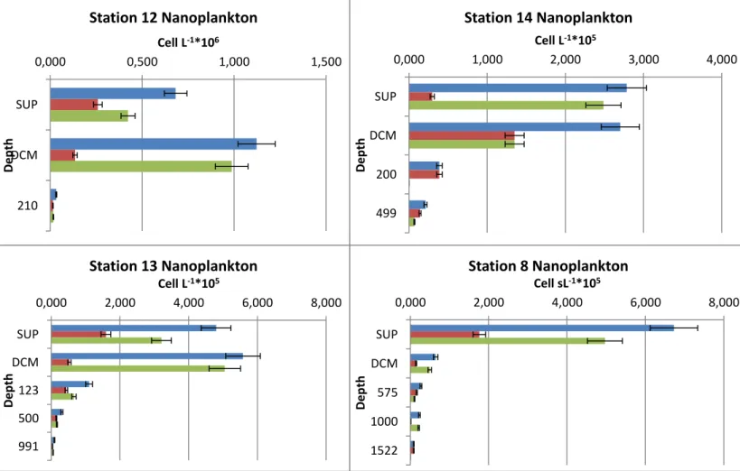
4.2.2.2 Total and class dimensional nanoplankton distribution

Bisagno transect

Stations 14 and 8 show a decrease in abundances from the surface layer to the bottom-depth; stations 12 and 13 show an increase in abundances from the surface layer to the DCM and then a decrease in abundances toward the bottom. The peaks of abundances of pigmented nanoplankton in correspondence of the DCM is found at stations 12 and 13. For dimensional classes graphs of all stations show higher abundances of pigmented cells compared to heterotrophic cells, especially in the surface and DCM layer.

Figure 4.2.2.2 a: blue column refers to total nanoplankton, red column to HNF, green column to PNF 0,000 0,500 1,000 1,500 SUP DCM 210 Cell L-1_*106 D ep th Station 12 Nanoplankton 0,000 1,000 2,000 3,000 4,000 SUP DCM 200 499 Cell L-1_*105 D e p th Station 14 Nanoplankton 0,000 2,000 4,000 6,000 8,000 SUP DCM 123 500 991 Cell L-1_*105 D ep th Station 13 Nanoplankton 0,000 2,000 4,000 6,000 8,000 SUP DCM 575 1000 1522 Cell sL-1_*105 D e p th Station 8 Nanoplankton

(37)

Figure 4.2.2.2 b: blue-filled column refers to cells of 5-10µm size, dot-filled column to cells of 3-5µm size, line-filled column to cells of 2-3µm size.

0,00 1,00 2,00 3,00 4,00 5,00 6,00 7,00 P E P E P E SU P DC M 21 0 Cell L-1_*105

0,00 0,20 0,40 0,60 0,80 1,00 1,20 1,40 P E P E P E P E SU P DC M 20 0 49 9 Cell L-1_*105

0,00 1,00 2,00 3,00 4,00 P E P E P E P E P E SU P DC M 12 3 50 0 99 1 Cell L-1_*105

0,00 0,50 1,00 1,50 2,00 2,50 3,00 3,50 P E P E P E P E P E SU P DC M 57 5 10 00 15 22 Cell L-1_*105

(38)

4.2.2.2 Total and class dimensional nanoplankton biomass

distribution Bisagno transect

The biomass distribution has the same trend of abundances distribution.

Figure 4.2.2.2 a : blue-filled column refers to HNF, line-filled to PNF

0 2 4 6 8

SUP

DCM

210

mg C Cell-1

0 0,5 1 1,5 2 2,5 SUP DCM 200 499 mg C Cell-1

0 1 2 3 4 5 SUP DCM 123 500 991 mg C Cell-1

0 2 4 6 8 SUP DCM 575 1000 1522 mg C Cell-1

(39)

Class dimensional biomass of nanoplankton graphs show higher values of >5 µm class compared to the abundances’ graphs, slight decrease of 3-5 µm class and great decrease of 2-3 µm class importance relatively to abundances’ graphs.

Figure 4.2.2.2 b :blue-filled column is referred to cells size 5-10µm, dot-filled column is referred to cells size 3-5µm, line-filled column is referred to cells size 2-3µm

0,00 1,00 2,00 3,00 4,00 HNF PNF HNF PNF HNF PNF SU P 12 0 21 0 mg C L-1

0,00 0,20 0,40 0,60 0,80 1,00 HNF PNF HNF PNF HNF PNF HNF PNF SU P 62 20 0 49 9 mg C L-1

0,00 0,50 1,00 1,50 2,00 2,50 HNF PNF HNF PNF HNF PNF HNF PNF HNF PNF SU P 43 12 3 50 0 99 1 mg C L-1

0,00 1,00 2,00 3,00 4,00 HNF PNF HNF PNF HNF PNF HNF PNF HNF PNF SU P 23 0 57 5 10 00 15 22 mg C L-1

(40)

4.2.3 Conjoint abundances’ distribution Bisagno transect

We found conjoint cells also in bottom-depth layer of station 12; there is not any clear trend from surface to deeper layers. Peaks of abundance are reached for surface at station 14, at DCM at station 13.

Figure 4.2.3: purple column refers to conjoint cells

0,000 2,000 4,000 6,000 8,000 10,000 SUP DCM 210 Cell L-1_*104 Station 12 Conjoint 0,000 0,500 1,000 1,500 2,000 2,500 SUP DCM 200 499 Cell L-1_*105 Station 14 Conjoint 0,000 20,000 40,000 60,000 SUP DCM 123 500 991 Cell L-1_*104 Station 13 Conjoint 0,000 1,000 2,000 3,000 4,000 SUP DCM 575 1000 1522 Cell L-1_*104 Station 8 Conjoint

(41)

4.3.1 Picoplankton abundances distribution Polcevera transect

All stations show an increase in abundances from yhe surface layer to the DCM, except station 3; the peak of abundance of phototrophic picoplankton in

correspondence of DCM is found at all stations except station 3.

Figure 4.3.1: blue column refers to total picoplankton, red column to heterotrophic picoplankton, green column is to phototrophic picoplankton 0 2 4 6 SUP DCM 226 Cell L-1_*108 D e p th Station 1 Picoplankton 0,000 2,000 4,000 6,000 8,000 SUP DCM 200 498 Cell L-1_*108 D e p th Station15 Picoplankton 0,000 2,000 4,000 6,000 SUP DCM 300 496 843 Cells L-1_*108 D ep th Station 2 Picoplankton 0,000 2,000 4,000 6,000 8,000 SUP DCM 500 1000 1482 Cells L-1_*108 D e p th Station 3 Picoplankton 0,000 2,000 4,000 6,000 8,000 SUP DCM 487 1000 1500 1950 Cells L-1_*108 D ep th Station 4 Picoplankton

(42)

4.2.3.1 Picoplankton biomass distribution Polcevera transect

The biomass distribution has the same trend of abundances’ distribution.

Figura 4.2.3.1 : HB refers to heterotrophic bacteria, Photopico to phototrophic picoplankton

0,00 2,00 4,00 6,00 8,00 10,00 HB Photopico HB Photopico HB Photopico SU P DC M 22 6 mg C L-1

0,00 5,00 10,00 HB Photopico HB Photopico HB Photopico HB Photopico SU P DC M 20 0 49 8 mg C L-1

0,00 2,00 4,00 6,00 8,00 10,00 12,00 HB Photopico HB Photopico HB Photopico HB Photopico HB Photopico SU P DC M 50 0 10 00 14 82 mg C L-1

0,00 5,00 10,00 HB Photopico HB Photopico HB Photopico HB Photopico HB Photopico HB Photopico SU P DC M 48 7 10 00 15 00 19 50 mg C L-1