e n z o a l b e r t o c a n d r e va
A U N I TA R Y A P P R O A C H T O I N F O R M AT I O N A N D E S T I M AT I O N T H E O R Y I N D I G I TA L
C O M M U N I C AT I O N S Y S T E M S
Ph.D. Programme in Electronics, Computer Science and Telecommunications - XXII Cycle
Department of Electronics, Computer Science and Systems - DEIS Alma Mater Studiorum - Università di Bologna
A U N I TA R Y A P P R O A C H T O I N F O R M AT I O N A N D
E S T I M AT I O N T H E O R Y I N D I G I TA L C O M M U N I C AT I O N
S Y S T E M S
e n z o
a l b e r t o
c a n d r e va
Ph.D. Programme in Electronics, Computer Science and Telecommunications
-XXII Cycle
Coordinator: Prof. Paola Mello
Supervisor: Prof. Giovanni E. Corazza
SSD: ING-INF/03
Department of Electronics, Computer Science and Systems - DEIS
Alma Mater Studiorum - Università di Bologna
Enzo Alberto Candreva: A Unitary Approach to Information and Estima-tion Theory in Digital CommunicaEstima-tion Systems, Department of Electronics, Computer Science and Systems - DEIS, Alma Mater Studiorum - Uni-versità di Bologna © March 2010
A B S T R A C T
This thesis presents the outcomes of a Ph.D. course in telecommunica-tions engineering. It is focused on the optimization of the physical layer of digital communication systems and it provides innovations for both multi- and single-carrier systems. For the former type we have first addressed the problem of the capacity in presence of several nuisances. Moreover, we have extended the concept of Single Frequency Network to the satellite scenario, and then we have introduced a novel concept in subcarrier data mapping, resulting in a very low Peak-to-Average-Power Ratio (PAPR) of the Orthogonal Frequency Division Multiplexing (OFDM) signal.
For single carrier systems we have proposed a method to optimize constellation design in presence of a strong distortion, such as the non linear distortion provided by satellites’ on board high power amplifier, then we developed a method to calculate the bit/symbol error rate related to a given constellation, achieving an improved accuracy with respect to the traditional Union Bound with no additional complexity. Finally we have designed a low complexity Signal-to-Noise Ratio (SNR) estimator, which saves one-half of multiplication with respect to the Maximum Likelihood (ML) estimator, and it has similar estimation accuracy.
S O M M A R I O
Questa tesi presenta i risultati ottenuti durante un dottorato di ricerca in ingegneria delle telecomunicazioni. Oggetto di studio è stato il livello fisico dei sistemi di trasmissione numerica, e sono state proposte innovazioni per i sistemi multi-portante e a portante singola. Nel primo caso è stata valutata la capacità di un sistema affetto da varie non idealità. In seguito l’idea di Single Frequency Network è stata estesa dall’ambito terrestre a quello satellitare, ed infine è stata presentata una nuova tecnica per effettuare il mapping da bit a simboli, che ha permesso di raggiungere fattori di cresta particolarmente bassi per il segnaleOFDM(Orthogonal Frequency Division Multiplexing).
Per i sistemi a portante singola, è stato proposto un metodo per ottimizare il progetto delle costellazioni in presenza di una forte distor-sione, quale ad esempio la distorsione non lineare dovuta agli ampli-ficatori di potenza a bordo dei satelliti. In seguito è stato sviluppato un metodo per calcolare la probabilità d’errore per bit e per simbolo riferita ad una data costellazione. Tale metodo ha la stessa complessità dello Union Bound ma risulta essere più accurato. Infine si è progettato uno stimatore di rapporto segnale-rumore, che permette il risparmio di metà delle moltiplicazioni rispetto al tradizionale stimatore a massima verosimiglianza, ma che mantiene prestazioni di stima comparabili.
O R I G I N A L C O N T R I B U T I O N S
This thesis presents original contributions in different fields. For the Orthogonal Frequency Division Multiplexing (OFDM) signal, the author has extended capacity evaluation in correlated fading to the case of discrete subcarrier constellations and channel estimation errors. This analysis provided a rule to optimize the number of pilot subcarri-ers, whose outcomes are presented in the following. Regarding Single Frequency Satellite Networks (SFSNs), the author contributed to the problem statement and to the numerical computations involved, while for Quasi-Constant EnvelopeOFDM, the author contributed in devising Peak-to-Average-Power Ratio (PAPR) reduction methods for the new data mappings. The methods hereby presented can be seen as a broa-dening of already known methods, but they required a new parameter optimization.
For the case of single-carrier system and signal, the author extended a method used for the Additive White Gaussian Noise (AWGN) to non-linear channel, obtaining the optimal constellation, in the sense of the minimum symbol error rate. These optimized constellations are shown to be resemblant of those applied in digital satellite communications, thus the contribution of the author was a theoretical justification of a concept known from an intuitive point of view. Moreover, the author developed a new bound on the error probability of the detection of signals corrupted byAWGN. This bound is tighter than the Union Bound, having the same complexity, and never exceeds the value of 1, returning thus a meaningful estimate of a probability. Finally, the author invented a reduced complexity Signal-to-Noise Ratio (SNR) estimator, which can save one half of the multiplications while retaining a satisfactory accuracy. A paper presenting thisSNRestimator has been awarded a Best Student Paper Award.
P U B L I C AT I O N S
Some proofs and figures have appeared previously in the following publications:
1. E.A. Candreva, G.E. Corazza, and A. Vanelli-Coralli, On the Opti-mization of Signal Constellations for Satellite Channels, Proceedings of International Workshop on Satellite and Space Communica-tions 2007 (IWSSC2007), September 12-14, 2007, Salzburg, Austria, pp.299-303;
2. E.A. Candreva, G.E. Corazza, and A. Vanelli-Coralli, On the Con-strained Capacity of OFDM in Rayleigh Fading Channels, Proceedings of International Symposium on Spread Spectrum Techniques and Applications 2008 (ISSSTA 2008), Bologna, Italy, August 2008;
3. E.A. Candreva, G.E. Corazza, and A. Vanelli-Coralli A Reduced Complexity SNR Estimator, Proceedings of the 29th AIAA Interna-tional Communications Satellite Systems Conference, ICSSC 2009, Edinburgh, UK, June 2009 (received the best student paper awa r d);
4. G.E. Corazza, C. Palestini, E.A. Candreva, and A. Vanelli-Coralli The Single Frequency Satellite Network Concept: Multiple Beams for Unified Coverage, GLOBECOM 2009, Hawaii, USA, December 2009; 5. E.A. Candreva, G.E. Corazza and A. Vanelli-Coralli A Tighter Upper Bound on the Error Probability of Signals in White Gaussian Noise, to be submitted to ASMS 2010;
6. F. Bastia, C. Bersani, E.A. Candreva, S.Cioni, G.E. Corazza, M. Neri, C. Palestini, M. Papaleo, S. Rosati, and A Vanelli-Coralli, LTE Air Interface over Broadband Satellite Networks, EURASIP Journal on Wireless Communications and Networking, Vol. 2009;
7. E.A. Candreva, G.E. Corazza, and A. Vanelli Coralli A Reduced Complexity Data-Aided SNR Estimator to be submitted to IEEE Communication Letters;
8. S. Rosati, E.A. Candreva, G.E. Corazza and A.Vanelli-Coralli OFDM Schemes with Quasi-Constant Envelope, to be submitted to IEEE Transactions on Communications;
9. E.A. Candreva, G.E. Corazza and A. Vanelli-Coralli, Pilot Design and Optimum Information Transfer in OFDM Systems, to be sumbit-ted to IEEE Transactions on Communications.
Si è così profondi, ormai, che non si vede più niente. A forza di andare in profondità, si è sprofondati. Soltanto l’intelligenza, l’intelligenza che è anche "leggerezza", che sa essere "leggera" può sperare di risalire alla superficialità, alla banalità. L. Sciascia, Nero su Nero, Einaudi, 1979
A C K N O W L E D G M E N T S
This document is a PhD Thesis, thus it is not the best place for all possible kinds of sentimental acknowledgments. However, the author would like to mention that he is deeply indebted to Professor Giovanni E. Corazza and to the bright fellows and trusted friends in his research group. The author did enjoy three years of interesting discussion about a very broad range of topics, often unrelated to Telecommunications. The author has learnt a lot in these three years, and he hopes to have contributed to the achievements of Digicomm Research Group.
C O N T E N T S
i i n n ovat i o n s i n m u lt i-carrier systems 1
1 o f d m c a pa c i t y i n p r e s e n c e o f i m pa i r m e n t s 3
1.1 Introduction 3
1.2 System Model 3
1.3 Capacity of Discrete-Input Continuous-Output Chan-nels 4
1.3.1 Constrained capacity for single-carrier systems in Additive White Gaussian Noise (AWGN) 4
1.3.2 Capacity in Fading Channels 6
1.4 Capacity of OFDM systems 6
1.4.1 Theoretical Background 6
1.4.2 Results 8
1.5 Impact of Channel Estimation Errors over OFDM Capac-ity 12
1.5.1 Performance Degradation 12
1.5.2 Pilot Field Design 13
1.5.3 Numerical Results 13 1.6 Conclusions 15 2 s i n g l e f r e q u e n c y s at e l l i t e n e t w o r k s 17 2.1 Introduction 17 2.2 OFDM and CDD 19 2.3 SFN over Satellites 20
2.3.1 Multi-beam coverage for Single Frequency Satel-lite Network (SFSN) 20
2.3.2 Spot Beam Radiation Diagram 21
2.3.3 Multi-Beam Cyclic Delay Diversity (MBCDD) Ap-proximated Transfer Function 22
2.3.4 Parameter Optimization 23
2.4 SFSN Capacity 25
2.5 First Proof of Concept for SFSN 26
2.6 Link Budget Analysis 27
2.7 Numerical Evaluation 29
2.8 SFSN: Pros and Cons 29
2.9 Conclusions 30
3 q ua s i-constant envelope ofdm 33
3.1 Introduction 33
3.2 Context System Model 34
3.2.1 Nonlinear Distortion 34
3.2.2 Orthogonal Frequency Division Multiplexing (OFDM) signal 36
3.3 Rotation-Invariant Subcarrier Mapping 38
3.3.1 Constellation design 38
3.3.2 Spherical Active Constellation Extension (ACE) 38
3.3.3 Extensions 39 3.4 AWGN Detectors 40 3.5 Numerical Results 41 3.6 Conclusions 45 4 f u r t h e r d e v e l o p m e n t s o f t h e p r e s e n t e d w o r k 47 xi
xii c o n t e n t s ii i n n ovat i o n s i n s i n g l e c a r r i e r s y s t e m s 49 5 o p t i m i z at i o n o f c o n s t e l l at i o n s ov e r n o n-linear chan-n e l s 51 5.1 Introduction 51 5.2 System Model 52 5.2.1 Received Signal 52 5.2.2 Error Probability 53 5.3 Proposed Algorithm 54 5.3.1 Description 54 5.3.2 Convergence 55 5.3.3 Discussion 56 5.4 Results 56 5.5 Conclusions 57 6 a t i g h t e r u p p e r b o u n d f o r e r r o r p r o b a b i l i t y o f s i g -na l s i n aw g n 61 6.1 Introduction 61
6.2 SER Computation for 2-dimensional Signal Constella-tions 62
6.2.1 Signal Model 62
6.2.2 Bonferroni inequalities 63
6.2.3 Proposed Upper Bound 64
6.2.4 Numerical Results 66
6.3 Codeword Error Rate Computation for Binary Block Codes 68 6.3.1 Signal Model 68 6.3.2 Proposed Bound 70 6.3.3 Numerical Results 70 6.4 Conclusions 70 7 a r e d u c e d c o m p l e x i t y s i g na l t o n o i s e r at i o e s t i m a -t o r 75 7.1 Introduction 75
7.2 Signal-to-Noise Ratio Estimators 75
7.3 Analytical Model of the Reduced Complexity Estima-tor 77
7.4 Non-Ideal Phase Reference 78
7.5 Numerical Results 79 7.6 Conclusions 80 8 f u r t h e r d e v e l o p m e n t s o f t h e p r e s e n t e d w o r k 83 iii a p p e n d i x 85 a o n t h e e f f i c i e n c y o f pa p r r e d u c t i o n m e t h o d s i n s at e l -l i t e o f d m 87 a.1 Introduction 87
a.2 PAPR Reduction Techniques 87
a.2.1 Active Constellation Extension 88
a.2.2 Tone Reservation 88
a.2.3 Selected Mapping 89
a.3 Performance Results 89
L I S T O F F I G U R E S
Figure 1 Constrained Capacity as a function of Signal-to-Noise Ratio (SNR) for Quaternary Phase Shift Keying (QPSK), 8 Phase Shift Keying (PSK), 16 Quadrature Amplitude Modulation (QAM). 5
Figure 2 Constrained Capacity as a function of SNR for QPSK, 8PSKand 16QAMwith Rayleigh fading and comparison toAWGNchannel. 6
Figure 3 Instantaneous Capacity ofOFDMsystems employ-ingQPSK, 8PSK16QAMand its comparison with Shannon-predicted capacity. Es/N0= 0dB. 9
Figure 4 Cumulative Density Function (CDF) of the instan-taneous capacity ofOFDMsystems employingQPSK, 8PSK16QAMand its comparison with Shannon-predicted capacity. Es/N0= 0dB. 9
Figure 5 Instantaneous Capacity ofOFDMsystems employ-ingQPSK, 8PSK16QAMand its comparison with Shannon-predicted capacity. Es/N0= 3dB. 10
Figure 6 CDFof the instantaneous capacity of OFDM sys-tems employingQPSK, 8PSK16QAMand its com-parison with Shannon-predicted capacity. Es/N0=
3dB. 10
Figure 7 Instantaneous Capacity ofOFDMsystems employ-ingQPSK, 8PSK16QAMand its comparison with Shannon-predicted capacity. Es/N0= 6dB. 11
Figure 8 CDFof the instantaneous capacity of OFDM sys-tems employingQPSK, 8PSK16QAMand its com-parison with Shannon-predicted capacity. Es/N0=
6dB. 11
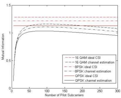
Figure 9 Optimization of the number of pilot subcarriers, Es/N0= 0dB. 14
Figure 10 Optimization of the number of pilot subcarriers, Es/N0= 3dB. 14
Figure 11 Optimization of the number of pilot subcarriers, Es/N0= 6dB. 15
Figure 12 3dB footprint of 400 Geostationary Earth Orbit (GEO) satellite beams over a 650.000 km2coverage area. Numerical parameters as in Table1. 18
Figure 13 Cyclic Delay Diversity (CDD)OFDMtransmitter. 19
Figure 14 Broadcasting over Europe: single beam, linguistic beams, local beams. 20
Figure 15 Spot beam radiation and mask for T = 20dB and p = 2. 22
Figure 16 Overall transfer function for three beams and N = 1, 2, 3, 20 paths each beam as a function carrier index. 23
Figure 17 Effective transfer function withoutMBCDD. Three overlapping beams. 23
Figure 18 Effective transfer function with MBCDD. Three overlapping beams. Non-optimized parameters. 24
xiv List of Figures
Figure 19 Effective transfer function with MBCDD. Three overlapping beams. Optimized parameters. 24
Figure 20 Capacity comparison in the three scenarios: single beam, two overlapping beams, three overlapping beams. 25
Figure 21 Capacity obtained in an area covered with six beams. 26
Figure 22 Snapshot of the capacity obtained in an area cov-ered with six beams. 27
Figure 23 Capacity comparison:SFSNvs. Single Beam Single Carrier. 30
Figure 24 Circularly simmetrical constellation. 39
Figure 25 Clover constellation. 40
Figure 26 Error Probability of Two Level Mapping. 42
Figure 27 Decision Regions for Clover Mapping. 42
Figure 28 Bit Error Probability for Clover Mapping. 43
Figure 29 Peak-to-Average-Power Ratio (PAPR) distribution for Two level and Clover Mappings. 43
Figure 30 Signal-to-Distortion Ratio (SDR) on Saleh High Power Amplifier (HPA) vs Input Back Off (IBO) for the proposed mappings. 44
Figure 31 SDRon Ideal Clipping (IC)HPAvsIBOfor the pro-posed mappings. 44
Figure 32 Bit Error Rate (BER) on SalehHPAatIBO= 0dB for the proposed mappings. 45
Figure 33 BER on IC HPA at IBO = 0 dB for the proposed mappings. 45
Figure 34 Optimal Signal Set for IBO = 8 dB, γ = 10 dB. 58
Figure 35 Optimal Signal Set for IBO = 12 dB, γ = 10 dB. 58
Figure 36 Optimal Signal Set for IBO = 16 dB, γ = 10 dB. 59
Figure 37 Optimal Signal Set for IBO = 16 dB, γ = 14 dB. 59
Figure 38 Constellation and bit mapping for 16-Amplitude-Phase Shift Keying (APSK), as prescribed in [30]. 66
Figure 39 Symbol error Probability for 16-APSK. 67
Figure 40 Constellation and bit mapping for 32-APSK, as prescribed in [30]. 67
Figure 41 Symbol error Probability for 32-APSK. 68
Figure 42 Codeword Error Probability for the BCH (63,24) code. 71
Figure 43 Codeword Error Probability for the BCH (63,30) code. 72
Figure 44 Codeword Error Probability for the BCH (63,36) code. 72
Figure 45 Codeword Error Probability for the BCH (63,39) code. 73
Figure 46 Maximum Likelihood (ML)SNREstimator. 76
Figure 47 Reduced ComplexitySNREstimator. 77
Figure 48 Normalized Mean Square Error (MSE) inAWGN only, Np= 64. 80
Figure 49 NormalizedMSEin presence of phase error, Np=
64. 80
Figure 50 NormalizedMSEinAWGNonly, Np= 1024. 81
Figure 51 NormalizedMSEin presence of phase error, Np=
1024. 81
Figure 52 Total Degradation for QPSK code-rate 1/5 and variousPAPRreduction techniques- 91
Figure 53 Total Degradation for QPSK code-rate 1/2 and variousPAPRreduction techniques- 92
Figure 54 Total Degradation for 16-QAMcode-rate 2/3 and variousPAPRreduction techniques- 92
L I S T O F TA B L E S
Table 1 Link budget for Single Beam andSFSNsystems. 28
Table 2 Values of α and β for the Saleh model. 36
Table 3 Spectra of the BCH codes used in simulations. 71
Table 4 Complexity comparison of two Data-AidedSNR circuits. 77
A C R O N Y M S
ACE Active Constellation Extension
ACI Adjacent Channel Interference
AGC Automatic Gain Control
APSK Amplitude-Phase Shift Keying
AWGN Additive White Gaussian Noise
BER Bit Error Rate
BPSK Binary Phase Shift Keying
CCDF Complementary Cumulative Density Function CDD Cyclic Delay Diversity
CDF Cumulative Density Function
CER Codeword Error Rate
CRB Cramer-Rao Bound
DFT Discrete Fourier Transform
DTH Direct to Home
EHF Extremely High Frequency
xvi a c r o n y m s
EIRP Effective Isotropic Radiated Power FFT Fast Fourier Transform
GEO Geostationary Earth Orbit HDTV High Definition Television
HPA High Power Amplifier
IBO Input Back Off
IC Ideal Clipping
IDFT Inverse Discrete Fourier Transform
IFFT Inverse Fast Fourier Transform
ISI Inter-Symbol Interference
MBCDD Multi-Beam Cyclic Delay Diversity
MIMO Multiple-Input Multiple-Output
MISO Multiple-Input Single-Output
ML Maximum Likelihood
MMSE Minimum Mean Square Error
MSE Mean Square Error
OBO Output Back Off
OFDM Orthogonal Frequency Division Multiplexing
PAPR Peak-to-Average-Power Ratio
pdf probability density function
PHY Physical Layer
PSK Phase Shift Keying
QAM Quadrature Amplitude Modulation
QPSK Quaternary Phase Shift Keying QoS Quality of Service
r.v. random variable
SDR Signal-to-Distortion Ratio
SDTV Standard Definition Television SER Symbol Error Rate
SFN Single Frequency Network
SFSN Single Frequency Satellite Network
SLM Selected Mapping
SNR Signal-to-Noise Ratio
STBC Space-Time Block Codes
TR Tone Reservation
Part I
I N N O VAT I O N S I N M U LT I - C A R R I E R
S Y S T E M S
𝟏
O F D M C A PA C I T Y I N P R E S E N C E O F I M PA I R M E N T S1.1 i n t r o d u c t i o n
The importance of Orthogonal Frequency Division Multiplexing (OFDM) is rapidly growing, because of its ability to cope with frequency-selective channels with simple equalization. This powerful multiplexing technique is being adopted on almost all new generation communica-tion standards, in the most various scenarios: wireline, digital television, mobile radio, and satellite. Although theOFDMis an established com-munication technique, the investigation and the analysis on this topic were essentially developed with the error rate as a target performance indicator. On the other hand, [21] presents an attempt to characterize OFDMfrom an information theoretic point of view, following a simpli-fied approach in order to assess the instantaneous capacity ofOFDM systems.
The aim of this chapter is to give a realistic characterization of the capacity of anOFDMsystem under frequency-selective Rayleigh fading, taking into account not only the correlation of fading amongst sub-channels (as in [21]), but also the discrete nature of the signal set for every sub-channel. A special form of Central Limit Theorem [13] is used in order to derive the overall system capacity. We show that the constrained capacity is Gaussian distributed, and we compute its mean and variance. With this method it is possible to have a reasonable analytical expression for the constrained capacity ofOFDM, and taking into account all the other overheads inOFDM(such as guard interval, pilot insertion, etc.) a realistic measure of the throughput available to the users is readily obtained.
The rest of this chapter is structured as follows: Section1.2presents
a brief description ofOFDMsystems and fading channels. Section1.3
describes the capacity of a discrete-input continuous-output channel, and Section1.4applies this result to the calculation of the overall system
capacity. Section 1.5 assesses the system capacity in the presence of
estimation errors, and the conclusions are presented in Section1.6
1.2 s y s t e m m o d e l
AnOFDMsystem [19] with N sub-carriers transmits in the n-th discrete time interval the data symbol xk,non the k-th sub-carrier, where xn,k∈
C belongs to a specific constellation {xi}Mi=1 with cardinality M and
k = 0, . . . , N − 1. Each subcarrier is assumed to have a bandwidth of ∆fand the total bandwidth is B = N∆f. The duration of each discrete time interval is T = ∆f1 , and the signal transmitted during the n-th time interval (composed by the superposition of the N modulated sub-carriers) is called the n-thOFDMsymbol.
The time-domain view of the n-thOFDM symbol is sn(t), for (n −
1)T < t⩽ nT and its samples are given by
sn,i= √1 N N−1∑ k=0 xk,nej2πikN, i = 0, . . . , N − 1 (1.1) 3
4 o f d m c a pa c i t y i n p r e s e n c e o f i m pa i r m e n t s
In other terms, Eq. (1.1) states thatOFDMmodulation is equivalent to
an Inverse Discrete Fourier Transform (IDFT) of the data symbol vector. The signal sn(t)is transmitted through a time-varying channel whose
impulse response is h(τ, t) and is further degraded by a complex Gaus-sian noise process with power spectral density N0.
The channel is assumed to be affected by a frequency-selective Rayleigh fading, and is described by the well known Jakes model [47].
In this model, h(t, τ) describes a wide-sense stationary with un-correlated, isotropic scattering. The delay autocorrelation function is supposed to be described as 1 2E [h(t, τ1)h ∗(t, τ 2)] = 1 τde −τ1τd δ(τ1− τ2) (1.2)
assuming thus an exponential delay power profile, with root mean square delay τd Then the k-th sub-channel gain during n-th block time
is H(nT , fk) = Hn,k where H(t, f) is the Fourier transform of h(t, τ)
with respect to the variable τ. From [47] the complex sub-channel gain can be written as Hn,k = pn,k+ jqn,k, where pn,k, qn,k ∼ 𝒩(0,12)
without any loss of generality.
The expression for the cross-correlation between the in-phase and quadrature components of the fading random variable (r.v.) for different time intervals or frequencies can be found in [47], but is necessary to give some detail about the distribution of|Hn,k|2, which is exponential
with
E[|Hn,k|2
]
= 1, Var[|Hn,k|2]= 1 (1.3)
and correlation coefficient [55] ρ(|Hn,k|2,|Hn,k+∆k|2) =
1
1 + (2π∆f∆kτd)2
(1.4) While the correlation coefficient in Eq. (1.4) is always different from zero,
following a pragmatic approach, the sub-channel gains on two fairly spaced sub-carriers can be considered independent if the correlation coefficient is significantly smaller than 1 (i.e. its value is less than a given threshold, like one tenth, or one hundredth).
Assuming perfect synchronization both in time and frequency, and a sufficient guard interval to avoid inter-block and inter-carrier interfer-ence, the receiver samples the received signal at rate B and performs a Discrete Fourier Transform (DFT) (recalling that Eq. (1.1) can be seen as
anIDFT) obtaining
Rk,n= Hk,nxk,n+ Nk,n (1.5)
where Nk,n is an Additive White Gaussian Noise (AWGN) sample, a
complex Gaussian variable having both real and imaginary part with zero mean and variance N0
2 .
1.3 c a pa c i t y o f d i s c r e t e-input continuous-output chan-n e l s
1.3.1 Constrained capacity for single-carrier systems inAWGN
The well known Shannon formula for Gaussian channels has to be in-tended as a theoretical upper bound on the capacity of communications
1.3 capacity of discrete-input continuous-output channels 5
systems. Pratical digital systems do not use Gaussian codebooks, they rather are constrained to emit symbols taken from a discrete set.
Based on this premise, the capacity of a communication systems has to be constrained, releasing the assumption of continuous input to the channel and assuming equiprobable signalling
The expression for this more realistic measure of capacity (which is usually referred to constrained capacity) can be found in [23,37] and, for a signal set whose cardinality is M its value is
I(X, Y) = log2M − 1 M M−1∑ i=0 E [ log2 ∑M−1 j=0 p(y|xj) p(y|xi) ] (1.6)
where averaging is performed with respect to p(y|xi), the conditional
pdf of the channel output y with respect to the input symbol xi. If the
only nuisance isAWGN, the conditional probability density functions are gaussian and the averaging operation (which is performed with respect to channel outputs) can be numerically evaluated with Gaussian quadrature formulas. Strictly speaking, Eq. (1.6) represents a mutual
information, not a capacity, but imposing the constraint of equiprobable signalling and discrete signal set, no best result can be achieved, so it is not improper referring to Eq. (1.6) as a constrained capacity. At a
first glance, Eq. (1.6) shows that the mutual information cannot reach
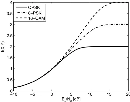
an infinite value, even in the case of an infinite signal-to-noise ratio, but it is bounded by log2M. As an example, Fig.1shows the behavior
of the mutual information as a function of signal-to-noise ratio for Quaternary Phase Shift Keying (QPSK), 8-Phase Shift Keying (PSK) and 16-Quadrature Amplitude Modulation (QAM).
−10 −5 0 5 10 15 20 0 0.5 1 1.5 2 2.5 3 3.5 4 E s/N0 [dB] I(X;Y) QPSK 8−PSK 16−QAM
6 o f d m c a pa c i t y i n p r e s e n c e o f i m pa i r m e n t s
1.3.2 Capacity in Fading Channels
The formula in Eq. (1.6) can be extended assuming the presence of
fading and perfect channel state information at the receiver, and it becomes:
I(X, Y|H) = log2M − 1 M⋅ M−1∑ i=0 E [ log2 ∑M−1 j=0 p(y|xj, h) p(y|xi, h) ] (1.7)
where h is a sample of the fadingr.v. H, and the average has to be performed with respect to both fading probability density function p(h), and p(y|xi, h), the probability density of channel output conditioned
to channel input and fading realization. Thus a double integral is required, and its evaluation is aided by Gaussian quadrature formulas. With the formulation of Eq. (1.7) the result is an average capacity, while
the instantaneous capacity is a random variable, dependent on the realization of the fadingr.v.
Fig.2compares the behavior of the mutual information as a function
of signal-to-noise ratio inAWGNand in a Rayleigh fading environment, modeled as in Section1.2. −10 −5 0 5 10 15 20 0 0.5 1 1.5 2 2.5 3 3.5 4 E s/N0 [dB] I(X;Y) QPSK AWGN QPSK fading 8−PSK AWGN 8−PSK fading 16−QAM AWGN 16−QAM fading
Figure 2: Constrained Capacity as a function ofSNRfor QPSK, 8 PSKand 16
QAMwith Rayleigh fading and comparison toAWGNchannel.
1.4 c a pa c i t y o f o f d m s y s t e m s 1.4.1 Theoretical Background
Given the capacity for every sub-carrier affected by fading and noise, as in Eq. (1.7), to calculate the instantaneous capacity for anOFDMsystem
it is necessary to recall an extension of the Central Limit Theorem for correlated random variables (r.v.s). There are various papers on this topic [2,13,28,29,71] but the most effective approach is reported in [13],based on the following theorem
1.4 capacity of ofdm systems 7
Theorem 1.4.1 Let {xj} be a sequence of random variables (r.v.s) with the
following properties 1. E [xj] = 0 2. 0 < σ2l ⩽ E[x2j]= σ2j ⩽ σ2u<∞ 3. 0 < β2 l ⩽ E [ |xj|3] = β2j ⩽ β2u<∞ 4. ∃ n <∞ : ρ(xi, xj) = 0 if |i − j| ⩾ n
then it follows that
M = lim N→∞ 1 N N ∑ i,j=1 E [xixj] ⩽ ∞ (1.8) and Y = lim n→∞ 1 √ N N ∑ i=1 xi (1.9)
is normally distributed with zero mean and variance M.
Hypotheses 2 and 3 assures that second- and third-order moments of ther.v.xjare bounded between two positive constants, respectively σ2l
and σ2
ufor the second-order moment and β2l and β2ufor the third-order
moment. Based on these hypotheses, M is finite and, although it can be simply upper-bounded by (2n + 1)σ2j, a more accurate representation is given by the evaluation of Eq. (1.8) which can be further simplified
as M = n ∑ j=−n E[x0xj] (1.10)
This theorem is fundamental in evaluating the capacity of anOFDM system: ther.v.xi in theorem1.4.1is Ci−E [Ci], where Ci andE [Ci]
are the capacity of the i-th sub-carrier and its mean, as given by Eq. (1.7)
(the verification that Ckfulfills the hypotheses of Theorem1.4.1is trivial
and may be obtained by numerical evaluation). Based on this premise, we have:
1 N N ∑ i=1 Ci∼ 𝒩 ⎛ ⎝E [C] , 1 N n ∑ j=−n σ2Cρ [j] ⎞ ⎠ (1.11)
where σ2C is the variance of Ci and ρ [j] is the correlation coefficient
between the capacity associated at two carriers separated by j∆f. In order to have a good estimation of the variance in Eq. (1.11) we
follow a pragmatic approach, that prevents the variance of suffering by numerical errors when ρ [j] is very low. Thus n, the number of correlation coefficients to be considered is given by
n =max{j : ρ [j] ⩾ 0.01} (1.12)
This truncation is not significant, because of the scaling coefficient 1/N in the expression of variance in Eq. (1.11), and, on the other hand,
8 o f d m c a pa c i t y i n p r e s e n c e o f i m pa i r m e n t s
A qualitative analysis of this result ensures that the Gaussian distri-bution will converge in probability to its mean value as the number of sub-carriers tends to infinity, as expected by the law of Large Numbers, in its weak formulation.
In other words, following an operational point of view, to evaluate the instantaneous capacity of anOFDMsystem, it is necessary to evaluate the mean and the variance of the capacity of a single sub-channel affected by AWGNand fading, and then the distribution of the instantaneous capacity can be obtained.
This approach in calculating the instantaneous capacity is different from the one followed in [21] and yields a mean capacity closer to actual values, since it releases the assumption of Gaussian signalling for each sub-channel.
Starting from this theoretically-predicted capacity, the actual capacity of an OFDM system can be derived, taking into account the guard interval, block duration, and the number of active carriers. Furthermore, the outage capacity of an OFDMsystem can be obtained, by fixing a capacity value which corresponds to a given value of the cumulative distribution of the mutual information.
1.4.2 Results
The numerical results are obtained assuming 2048 subcarriers spaced of 4464 Hz, a channel model as in Section1.2, with τm= 19ns. These
values for the numerical parameters are chosen to be compliant with the newly adopted DVB-T2 [33]. Each subcarrier is transmitted with equal energy Es, so the total transmitted energy is NEs. N, the number
of sub-carriers is assumed equal to 2048. The receivedSNRof the k-th sub-carrier is|Hn,k|2 ENs0.
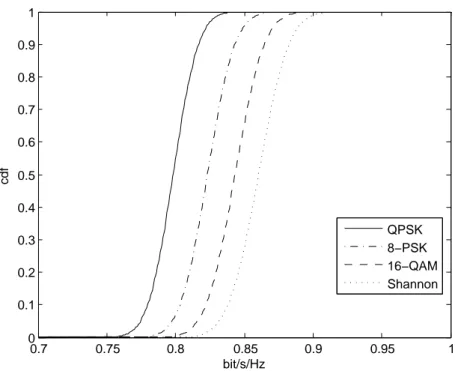
Fig.3shows the capacity prediction of a system employingQPSK, 8
PSK, and 16QAMat Es
N0 = 0 dBand these predictions are compared with
those based on Shannon formula. Fig.4shows the Cumulative Density
Function (CDF) of the instantaneous capacity in the same scenario.Fig.5
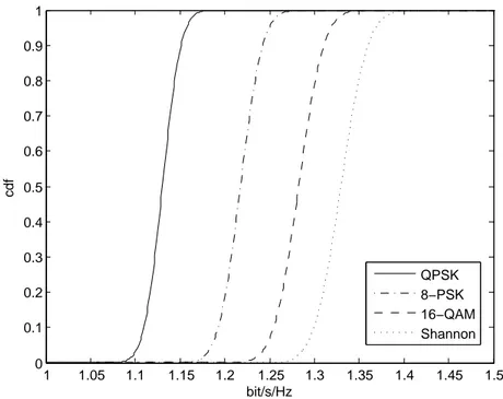
and Fig.6show the same comparison at Es
N0 = 3 dB, and finally, Fig.
7
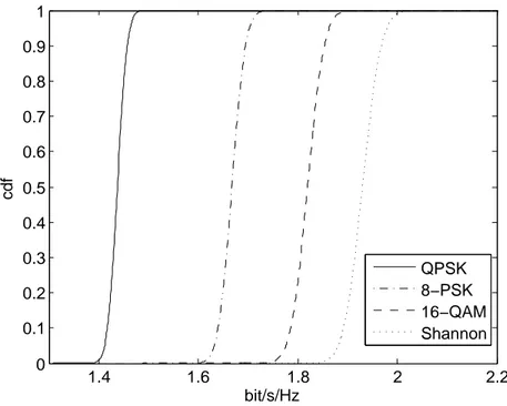
and Fig.8show the same comparison at Es
N0 = 6 dB.
It appears clearly from these results that the Shannon approach overestimates the instantaneous capacity of anOFDMsystem, while other measures, based upon constrained capacity, can be closer to the capacity of a real system. The difference between these estimates depends on signal-to-noise ratio, because the constrained capacity curves tend to "saturate" to a finite value, and on the environment, since the variance of the Gaussian distributions are a function of the memory of the channel: the higher the correlation, the higher the variance of the instantaneous capacity. By the same argument, if the carrier spacing is smaller, the sub-channels will be more correlated, thus increasing the variance.
Adaptive coding and modulation techniques with waterfilling appear to be attracting, thus, in order to exploit the variety of the instantaneous capacity rather than a conservative worst-case design.
1.4 capacity of ofdm systems 9 0.7 0.75 0.8 0.85 0.9 0.95 1 0 5 10 15 20 25 30 bit/s/Hz pdf QPSK 8−PSK 16−QAM Shannon
Figure 3: Instantaneous Capacity ofOFDMsystems employingQPSK, 8PSK16
QAMand its comparison with Shannon-predicted capacity. Es/N0=
0dB. 0.7 0.75 0.8 0.85 0.9 0.95 1 0 0.1 0.2 0.3 0.4 0.5 0.6 0.7 0.8 0.9 1 bit/s/Hz cdf QPSK 8−PSK 16−QAM Shannon
Figure 4:CDFof the instantaneous capacity ofOFDMsystems employingQPSK, 8PSK16QAMand its comparison with Shannon-predicted capacity. Es/N0= 0dB.
10 o f d m c a pa c i t y i n p r e s e n c e o f i m pa i r m e n t s 1 1.1 1.2 1.3 1.4 1.5 0 5 10 15 20 25 30 bit/s/Hz pdf QPSK 8−PSK 16−QAM Shannon
Figure 5: Instantaneous Capacity ofOFDMsystems employingQPSK, 8PSK16
QAMand its comparison with Shannon-predicted capacity. Es/N0=
3dB. 1 1.05 1.1 1.15 1.2 1.25 1.3 1.35 1.4 1.45 1.5 0 0.1 0.2 0.3 0.4 0.5 0.6 0.7 0.8 0.9 1 bit/s/Hz cdf QPSK 8−PSK 16−QAM Shannon
Figure 6:CDFof the instantaneous capacity ofOFDMsystems employingQPSK, 8PSK16QAMand its comparison with Shannon-predicted capacity. Es/N0= 3dB.
1.4 capacity of ofdm systems 11 1.3 1.4 1.5 1.6 1.7 1.8 1.9 2 2.1 0 5 10 15 20 25 30 bit/s/Hz pdf QPSK 8−PSK 16−QAM Shannon
Figure 7: Instantaneous Capacity ofOFDMsystems employingQPSK, 8PSK16
QAMand its comparison with Shannon-predicted capacity. Es/N0=
6dB. 1.4 1.6 1.8 2 2.2 0 0.1 0.2 0.3 0.4 0.5 0.6 0.7 0.8 0.9 1 bit/s/Hz cdf QPSK 8−PSK 16−QAM Shannon
Figure 8:CDFof the instantaneous capacity ofOFDMsystems employingQPSK, 8PSK16QAMand its comparison with Shannon-predicted capacity. Es/N0= 6dB.
12 o f d m c a pa c i t y i n p r e s e n c e o f i m pa i r m e n t s
1.5 i m pa c t o f c h a n n e l e s t i m at i o n e r r o r s ov e r o f d m c a pa c -i t y
1.5.1 Performance Degradation
Channel estimation forOFDMis now a well consolidated field, in which some very important results have been achieved, from both theoreti-cal and implementation point of view. From the theoretitheoreti-cal side, the optimal estimator has been derived, which is dependent on the assump-tions from the channel model, while from the practical standpoint, a big number of low complexity channel estimators have been designed, to strike a balance between estimation accuracy and computational complexity. In this section we will not derive the optimal estimators, rather we will focus on the differences between two commonly used approaches, and show their performances. A starting point in designing a channel estimator is given by the Maximum Likelihood (ML) criterion, for which the channel has unknown but deterministic parameters, i. e. the number of taps, their delays and amplitudes. This criterion allows to design a “rugged” estimator, which can operate under very different possible conditions. This estimator has a simple closed form for the variance of the estimation error, given by the Cramer-Rao Bound (CRB).
A different estimator, which leads to an improved performance, is based on the Minimum Mean Square Error (MMSE) criterion. In this case the channel response is regarded as a random quantity, whose probability distribution is known at the receiver. In this case the variance of the estimation error is lower than theCRB, because the hypotesis is different, and it has to be averaged not only over the observed data, but also on the channel realizations.
For further details on theOFDM channel estimation problems, the reader is referred to the very interesting results presented in [17,43,58, 59,77]. In what follows, we will present one of the main results collected in [58], i. e. the analytical expression for the variance of the estimation error for a multi-tap channel and OFDM signals. Assuming a noise variance of N0, a channel with L taps having energy σ2k, k = 1, . . . , L
and Np equispaced pilot subcarriers, we have
σ2ML= N0L
Np (1.13)
and
σ2MMSE= λ⋅ σ2ML (1.14)
where λ < 1 and it is given by
λ = 1 L L ∑ k=1 1 1 + N0 σ2 kNp (1.15)
It is important noticing that both σ2
MLand σ2MMSE are independent of
the subcarrier index, and they both confirm the intuitive feeling that the estimation accuracy degrades as the number of pilot tones decreases or the number of channel taps increases, for a givenSNR.
The next step to evaluate the impact of an imperfect channel estima-tion over the reliability of the transmission is to consider the effect of the estimation error over each subcarrier. As it is shown for example in
1.5 impact of channel estimation errors over ofdm capacity 13
[3,41,56], the effect of estimation error is twofold, since it causes both a reduction in the useful signal power and a contribution to the noise. Using the Shannon formula for the sake of simplicity, we can conclude that the capacity for a channel (here intended as the single subcarrier) affected by fading and non-ideal estimation is
C =EH,ε [ log2 ( 1 +(H − ε) 2E s N0+ ε2Es )] (1.16) where ε represents the estimation error.
1.5.2 Pilot Field Design
Based on the previous section, here we propose a method to optimize the pilot field design for anOFDMsystem. We will assume that the trans-mission is not continuous (i. e. it is performed in bursts) and the channel does not vary significantly over anOFDMsymbol. Futhermore we will assume that the pilot subcarriers are equispaced over the symbol, with the caveat in [58,59] that these locations are optimal if we assume no guard bands, otherwise the pilots shall be denser close to the guard bands. However, the assumption of equispaced pilots is instrumental for the analytical tractability of the problems, and still can provide a sort of “rule of thumb” for theOFDMsystem designer. Another impor-tant aspect in the pilot field design is the loss in throughput due to the subcarriers reserved for estimation. There is an obvious trade off between the accuracy and the loss in data rate: Eq. (1.13), (1.15) show an
inverse proportionality between the number of pilots and the variance of the estimation error. On the other hand, the greater the number of pilot subcarriers, the less the available subcarriers for data transmission. Given this point of view, it is natural to ask whether the number of pilot subcarriers shall be reduced to achieve what can seem an unsatisfactory estimation performance, leaving room, in this way, to an higher data transmission capability.
1.5.3 Numerical Results
In this section we show the optimization of the mean value in Eq. (1.11),
where the impact of estimation error is taken into account as in Eq. (1.16),
but assuming a discrete constellation, and the throughput loss due to channel estimation is considered by the insertion of a multiplicative factor
Nfft− Np
Nfft
(1.17) The channel is assumed to have 9 taps, as the channel models pre-sented in [70] to extend ITU channel models forOFDMsystems. Fig.9
shows the optimization of the number of pilot subcarriers, compared to the case of ideal channel state information, for an OFDM system employing QPSK, 8PSK, or 16QAM at Es
N0 = 0 dB. The red lines show
the case of ideal channel state information, where there is no estimation error neither throughput loss, while the black lines show the twofold impact of estimation errors on the subcarrier capacity, jointly with the throughput loss due by pilots insertion. Fig.10 show the same
opti-mization at Es
N0 = 3 dB, and finally, Fig.
11show the same optimization
at Es
14 o f d m c a pa c i t y i n p r e s e n c e o f i m pa i r m e n t s
Figure 9: Optimization of the number of pilot subcarriers, Es/N0= 0dB.
1.6 conclusions 15
Figure 11: Optimization of the number of pilot subcarriers, Es/N0= 6dB.
As it is shown in Fig.9,10,11, before the optimum, the number of
pilot subcarriers follows a law of diminishing returns: increasing by one the number of pilot tones leads to completely different performances whether the pilot tones number is already high or not. After the opti-mum number, the capacity will decrease, the higher theSNRthe steeper the decrease. In addition, the optimal number of pilot tones is highly dependent on the subcarrier modulation, and this is more evident for highSNR
1.6 c o n c l u s i o n s
This chapter presented an attempt to characterize the instantaneous capacity of anOFDMsystem, based on constrained capacity arguments and on the application of Central Limit Theorem. The results show that the unconstrained capacity formula is inaccurate in predicting the instantaneousOFDMcapacity, which depends on the modulation used and on the environment. The proposed approach based on Central Limit Theorem has an accuracy which is adequate for all practicalDFT sizes. Moreover, we have analyzed the capacity of anOFDMsystem in the presence of channel estimation errors. We have shown its effect on the capacity and derived a method to optimize the number of subcarriers reserved for channel estimation, maximizing the information transfer. This method can be useful inOFDM system design, giving at a first glance an approximation for the capacity of the system and the number of subcarrier to be assigned to pilots.
𝟐
S I N G L E F R E Q U E N C Y S AT E L L I T E N E T W O R K S2.1 i n t r o d u c t i o n
Satellite communications are experiencing very significant technical evolutions, which will be key in defining the role of satellites in future networks as a means to provide broadband access to the Internet over vast coverages. These changes have been enabled by new techniques and technologies: adaptive coding and modulation for the exploitation ofEHFbands, where several GHz of bandwidth are available; on board processing for in-space routing; large reflectors for multi-beam antennas with hundreds of spot beams; exploitation of digital beam-forming network concept; as well as significant improvements in on-board power amplification. All of this goes in the direction of maximizing system capacity and flexibility, and in general its effectiveness.
On the other hand, satellite broadcasting systems are naturally still focused on the objective of ensuring good coverage over vast areas and, consequently, have hardly exploited the new techniques potential. In fact, the classic Direct to Home (DTH) TV broadcasting satellite network provides service with a single beam typically operated in Ku
band, where hundreds of Standard Definition Television (SDTV) or High Definition Television (HDTV) channels can be carried over the entire service area. This is a successful paradigm with seemingly little room for innovation. More recent developments are in the area of Mobile Broadcasting to hand-held terminals, which require a lower frequency band with a more benign propagation environment, such as the S band. Since spectrum availability is here much scarcer (a maximum of 30MHz), it is necessary to use more efficiently the radio resource by exploiting frequency reuse. Considering European coverage, the satellite antenna pattern is typically organized into country-specific linguistic beams, which are grouped in clusters and assigned different frequency sub-bands, which can be reused in non-adjacent beams. Interference is caused by antenna side-lobes, which must be carefully kept under control. Unfortunately, the amount of reuse that can be achieved is small, and essentially determined by geographic configuration.
We propose here a radical increase in the fragmentation of the service area, both for fixed and for mobile applications, through the only exploitation of signal processing techniques over multi-beam antennas with hundreds of beams, also for broadcasting systems. Wherever content is identical in different beams (over a region, a country, or the entire service area) the same frequency band is used to realize a Single Frequency Satellite Network (SFSN), reminiscent of the Single Frequency Network (SFN) concept of terrestrial broadcasting systems, without resorting to any complexity increase in the antenna beamforming or any impact on the receiver. This architecture allows to have unprecedented flexibility in satellite broadcasting systems, as will be discussed shortly.
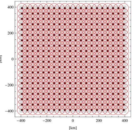
The reason why this idea has never been considered, or it has been rejected altogether, is that the signals carried by multiple beams in a SFSNmutually interfere in overlapping regions, inducing null-capacity zones wherever interference is destructive (see Fig.12for an example
18 s i n g l e f r e q u e n c y s at e l l i t e n e t w o r k s
of overlapping beams). If no countermeasures are taken, it proves impossible to provide uniform Quality of Service (QoS) throughout the service area. The innovative idea is to use Orthogonal Frequency Division Multiplexing (OFDM) [79] jointly with a new form of Multi-Beam Cyclic Delay Diversity (MBCDD) which creates synthetic multipath through the assignment of beam specific power delay profiles. In this way, frequency selectivity is introduced which results in sufficient diversity to avoid destructive interference, guaranteeing correct signal reception in the entire coverage area. Let us dwell briefly over the
-400 -200 0 200 400 -400 -200 0 200 400 @kmD @km D
Figure 12: 3dB footprint of 400GEOsatellite beams over a 650.000 km2coverage area. Numerical parameters as in Table1.
advantages and disadvantages of this approach. As for the main positive aspects, we consider the possibility to: use the same antenna pattern to provide broadcasting and broadband access, for triple play services; deliver efficiently local content and reuse that part of the spectrum extensively; shape precisely and adaptively the contour of beams by grouping spots; use power control selectively over those narrow beams where atmospheric conditions are bad; use a large number of small High Power Amplifiers (HPAs) instead of a few powerfulHPAsfor the same total power. On the down side, the use of OFDMandMBCDDis not as power efficient as conventional single-carrier techniques, and requires the use of channel equalizers in the receivers.
We believe that the advantages largely surpass the negative points. In this chapter, we describe how this idea takes practical form.
2.2 ofdm and cdd 19
2.2 o f d m a n d c d d
This section briefly describes the concept of Cyclic Delay Diversity (CDD) forOFDMsystems. As well known,OFDMis a multicarrier transmission technique, which splits the available spectrum into several narrowband parallel channels, corresponding to multiple sub-carriers modulated at a low symbol rate. TheOFDMsignal can be expressed as
s(t) = NFFT∑−1 k=0 xk⋅ ej2πk t T, −Tg⩽ t < T (2.1)
where xkare the complex-valued modulated data symbols, NFFT is the
total number of sub-carriers, T is the usefulOFDMsymbol time, Tg is
the guard interval duration. The guard interval is filled with a cyclic prefix to maintain orthogonality in multipath. Note that, in order to avoid adjacent channel interference, only Na< NFFT active carriers are
typically used.
Besides using the bandwidth very efficiently,OFDMguarantees high robustness against multipath delay spread, by allowing extremely sim-ple equalization in the frequency domain. So much so that we can increase artificially the channel delay spread by inserting TX-antenna specific cyclic delays.CDD[26], [25] is a Multiple-Input Multiple-Output (MIMO) scheme which allows to enhance the frequency selectivity by inserting additional multiple paths that would not naturally occur. Figure 13 illustrates the block diagram of an OFDM transmitter
ap-plying CDDon its NT X antennas. As shown, the same OFDM
modu-OFDM CP insertion CP insertion CP insertion
Figure 13:CDD OFDMtransmitter.
lated signal is transmitted over NT X antennas with an antenna
spe-cific cyclic shift. These shifts are indicated in the time domain by δi,
i = 1, ..., NT X− 1, δ ∈ Z and correspond to a multiplication by a phase
factor ψi(f) = e
−j2πf δi
NFFT. The latter, together with the normalization
term used to split equally the transmission power among the anten-nas, can be interpreted as due to the channel, leading to an equivalent overall channel transfer function reported in Eq. (2.2) [26]:
Heq(f, t) = 1 √ NT X NT X∑−1 i=0 ψi(f)⋅ Hi(f, t) (2.2)
where Hi(f, t) denotes the channel transfer function from the i-th
Multiple-20 s i n g l e f r e q u e n c y s at e l l i t e n e t w o r k s
Input Single-Output (MISO) case, and can obviously be extended to MIMO. Compared to the original propagation channel, the composite channel using CDD shows a much richer multi-path profile, i.e. an increased frequency diversity of the received signal due to the contribu-tion of theCDDtransmission scheme. This is especially useful on poor multi-path scenarios in combination with a powerful coding scheme.
Here we are interested in the potential of theCDDtechnique as ap-plied toSFSNs, in association to coded OFDM. Indeed, CDDhas been considered for Digital Video Broadcasting Terrestrial (DVB-T) applica-tions [25], but it has never been thought for satellite broadcasting. This is the contribution of the present chapter.
2.3 s f n ov e r s at e l l i t e s
Since the general aim of a broadcast service is to deliver the same signal to a very large audience dislocated over a wide area, one of the most effective solutions is to establish a satellite network. As clearly explained in the Introduction, the main novelty consists in providing broadcasting services through a multi-spot antenna synthesizing local beams, whereby several spots may be sending identical signals, to real-ize aSFSN. On board multi-beam antennas can be realized through the
Figure 14: Broadcasting over Europe: single beam, linguistic beams, local beams.
adoption of a Cassegrain reflector (which includes a parabolic primary mirror and a hyperbolic secondary mirror) and multi-feed horns; a sim-ilar structure to those utilized in Earth station antennas. More precisely, instead of having a single focal point where the feed must be located, the multi-beam antenna has a focal surface on which various feeds can be placed. Such an antenna system has a very compact structure and an adequate flexibility. The design of the reflectors position and feeders configuration realizes the desired beam geometry, in particular the beam overlapping areas on ground and the antenna side-lobes which are the main interference sources. Let us see how aSFSNcan be designed exploiting such a multi-beam antenna, through the combined use ofOFDMandMBCDD, performing signal processing at the gateway and assuming a transparent satellite transponder with beamforming.
2.3.1 Multi-beam coverage forSFSN
As mentioned before, combining signals coming from two or more over-lapping beams generates null-capacity zones wherever they interfere
2.3 sfn over satellites 21
destructively, causing deep fade events. If fading is frequency non-selective, this means that in certain points of the Earth surface no useful energy can be received. Obviously, this situation would be unacceptable for a broadcasting service since it is impossible to provide a uniform QoSthroughout the coverage area. The proposed strategy, relying on the adoption ofOFDMon the satellite link, is to applyMBCDDto each beam by imposing a specific delay profile that guarantees frequency selectivity over the signal bandwidth, generating a new source of di-versity. This frequency selectivity is beneficial since it can be exploited through codedOFDMand leads to an overall transfer function without any null zone in the entire bandwidth.
Consider the k-th beam. Let Hk(f, α, φ) be the channel transfer func-tion corresponding to this beam as seen by a point on Earth reached through a link with amplitude gain α and overall phase rotation φ. Clearly, α accounts for the path loss, while φ includes the initial phase imposed by the gateway transmitter, the phase rotation due to satellite beamforming and that due to propagation delay. Both α and φ are assumed to be constant over the entire signal bandwidth.
Let Hk
n = Hk(n∆f, αk, φk)be the transfer function coefficient
per-taining to the n-thOFDMsubcarrier, where the constants αkand φkare
implicit for notation simplicity. AssumeMBCDDis applied by creating Nksynthetic signal replicas at the gateway, each delayed by δi,kand
scaled by an amplitude coefficient Ai,k, for i = 1, . . . , Nk. Thus, the
n-th transfer function coefficient can be described as:
Hkn(αk, φk) = αkejφk Nk ∑ i=1 Ai,ke−j2πn mod(δi,k,NFFT ) NFFT (2.3)
where mod(a, b) indicates a module b. The 2Nk+ 1parameters
charac-terizing the power delay profile synthesized for the generic k-th beam give great flexibility, with plenty of degrees of freedom in selecting delays and amplitudes. These parameters can be optimized in the trans-mitter without any consequences at the receiver. The only constraint is that non selective fading per subcarrier should be guaranteed at all locations, in order to allow simple equalization; besides, channel esti-mation could became too challenging if the number of paths increases excessively.
Note that the application ofCDDis not realized with different anten-nas as in its original form, but through digital processing at the gateway. In this way the system results to be more flexible, since no limitation in the number of delays is introduced, independently of the number of antenna elements.
2.3.2 Spot Beam Radiation Diagram
In order to describe the radiation pattern of each beam, the model described in [78] and [16] has been used. The generic tapered-aperture antenna radiation pattern is reported in the following equation:
G(uk) = GM,k ( (p + 1)(1 − T ) (p + 1)(1 − T ) + T )2 ⋅ ( 2J1(uk) uk + 2p+1p! T 1 − T Jp+1(uk) up+1k )2 (2.4)
22 s i n g l e f r e q u e n c y s at e l l i t e n e t w o r k s
where GM,k is the maximum gain for the k-th beam, p is a design
parameter, T is the aperture edge taper, Jp(u) is the Bessel function
of the first kind and order p, uk = πdλasin θk, da,k is the effective
antenna aperture for the k-th beam, and λ is the wavelength. Note that in the following, the mask corresponding to G(uk)with T = 20dB and
p = 2, depicted in Fig.15, has been used. For simplicity, a flat model of
the Earth surface has been assumed, which is sufficiently accurate for beams which are not too large and not far from the sub-satellite point.
5 10 15 20 25 -80 -60 -40 -20 u G[dB] 5 10 15 20 25 -80 -60 -40 -20 u G[dB]
Figure 15: Spot beam radiation and mask for T = 20dB and p = 2.
2.3.3 MBCDDApproximated Transfer Function
Now we are in the position to evaluate the overall effect of beam superposition. Let NBbe the number of overlapping beams insisting
on a specific location with the same transmitted power, and Hnbe the
overall transfer function coefficient corresponding to the n-th subcarrier. Note that, at any location all αk coefficients are identical for any k;
therefore, only φkneeds to be explicit. It holds
Hn= Hn(φ1, . . . , φNB) = NB ∑ k=1 √ G(uk)Hkn(φk) (2.5)
The collection of NFFT channel coefficient forms the overall transfer
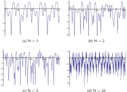
function over the signal bandwidth. Fig.16shows a snapshot of this
overall transfer function obtained with three overlapping beams having 1, 2, 3, 20 paths at the same power level for NFFT = 2048. Note that,
as desired, frequency selectivity is obtained, which enables ourSFSN architecture, at the price of the introduction of channel coding and equalization.
Since theOFDMsignal experiences a frequency selective channel, we need to introduce a figure that can represent the effective performance obtained over the entire band. We elect to use the approximated transfer function, ¯H, defined as the average of the absolute values of the channel transfer coefficients: ¯ H = 1 NFFT N∑FFT n=1 |Hn| (2.6)
Note that this function is an approximation of the merit figure shown in the following, which is representative of system performance. Fig.17
2.3 sfn over satellites 23 500 1000 1500 2000 -15 -10 -5 5 (a) N = 1 500 1000 1500 2000 -20 -15 -10 -5 5 (b) N = 2 500 1000 1500 2000 -25 -20 -15 -10 -5 5 (c) N = 3 500 1000 1500 2000 -40 -30 -20 -10 10 (d) N = 20
Figure 16: Overall transfer function for three beams and N = 1, 2, 3, 20 paths each beam as a function carrier index.
0 2 4 6 0 2 4 6 -40 -30 -20 -10 0 10
H
Ф1 Ф2Figure 17: Effective transfer function withoutMBCDD. Three overlapping beams.
φ3, and variable φ1 and φ2. The overlapping beams are assumed
to be at the same power level, withoutMBCDD. Note that for certain combinations of phases the transfer function of the channel without MBCDDpresents deep fades of the effective transfer function, which correspond to a null-capacity zone. On the other hand Fig.18shows
that these fades are resolved with the introduction of MBCDD, even without a specific optimization procedure, that will be described in the following.
2.3.4 Parameter Optimization
The optimized design of the delay profile have not only to avoid signal cancellation for any possible phase shift in the coverage area, but also to minimize the fluctuations of the effective transfer function. The worst case in terms of beam overlap is given by the three beam cluster structure. This means that three typical reception conditions have to be analyzed in order to optimize the provided QoS: one beam, two
24 s i n g l e f r e q u e n c y s at e l l i t e n e t w o r k s 0 2 4 6 0 2 4 6 -10 -5 0 5 10
H
Ф1 Ф2Figure 18: Effective transfer function withMBCDD. Three overlapping beams. Non-optimized parameters.
overlapping beams, and three overlapping beams. Interference coming from the other beams can be neglected. A deterministic or a statistical design can be followed in order to pursue the optimization. To reduce the number of degrees of freedom, it is possible to assume uniform amplitudes, Ai,k= A∀ i, k, and equally spaced paths, i.e. δi,k= i⋅ δ0,k,
under the fundamental requirement δ0,1∕= δ0,2∕= δ0,3. Moreover, these
three parameters can be optimized through the following expression: (δ0,1, δ0,2, δ0,3)opt= argmin δ0,1,δ0,2,δ0,3 ¯ Hmax− ¯Hmin (2.7) where ¯ Hmax = max φ1,φ2,φ3 (¯ H) ¯ Hmin= min φ1,φ2,φ3 (¯ H) (2.8) It can be shown that best results are obtained when the following three quantities
mod(δ0,1, NFFT), mod(δ0,2, NFFT), mod(δ0,3, NFFT)
are incommensurable. Fig.19shows an optimized (flat) effective transfer
function with incommensurable delays.
0 2 4 6 0 2 4 6 -10 -5 0 5 10
H
Ф1 Ф2Figure 19: Effective transfer function withMBCDD. Three overlapping beams. Optimized parameters.
2.4 sfsn capacity 25
2.4 s f s n c a pa c i t y
In this section we introduce theSFSNcapacity in information theoretic terms. Let P/N be the signal-to-noise ratio over a sub-carrier that would be experienced by a receiver in the absence of self-interference generated by CDDand with an isotropic antenna. Thus, in any specific location the capacity can be obtained as [7]:
C = Na ∑ n=1 log ( 1 +FnP N ) (2.9)
where Fn=|Hn|2forMBCDD, while in the case of a single beam Fnonly
accounts for the antenna gain at the specific location. This function will be used to assess the performance of aSFSNsystem.
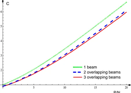
Now we will useSFSNcapacity shown in Eq. (2.9) to provide an initial
comparison between the single and multiple beam cases. In order to ensure fairness, the capacity is estimated assuming to have the same Effective Isotropic Radiated Power (EIRP) available in the two cases. This is reasonable because with multiple beams the antenna gain increases but the beam power decreases. A fair comparison is difficult because the geometry of single-beam/multi-beam coverages are quite different. Let us make a simple assumption which favors completely the single beam case, by placing the user at the sub-satellite point for the single beam case and in the middle point of beam-overlapping regions for the multi-beam case. The capacity obtained in these conditions is shown in Fig.20. Even in this extreme case, it can be seen that theMBCDDcapacity
5 10 15 20 2 3 4 5 6 3 overlapping beams 2 overlapping beams 1 beam P/N C
Figure 20: Capacity comparison in the three scenarios: single beam, two over-lapping beams, three overover-lapping beams.
is not far from the best case of single beam capacity, which is a good and somewhat unexpected result. The comparison would be even more favorable toMBCDDif the average capacity of the entire service area, or the worst case, would be considered. In any case, it is necessary to optimize the on-board antenna radiation diagram (beam apertures and centers) in order to maximize the flatness and fairness of the received power in the entire region.
26 s i n g l e f r e q u e n c y s at e l l i t e n e t w o r k s
2.5 f i r s t p r o o f o f c o n c e p t f o r s f s n
The design of the on-board antenna should be aimed at producing a uniform QoS across the entire service area. We report here a few results obtained in different beam geometry scenarios. The following assumptions have been used:
• NFFT = 2048
• Uniform spaced delays, δi= i⋅ δ0
• Number of multiple paths on each beam Ni equal to 2
• Uniform amplitude delay profile Ai= Awithin the same beam
• Same amplitude delay profile among different beams, A1= A2=
A3
• Incommensurable delays
• Effective antenna aperture daequal to 1.4 m for each beam
• Fixed NP equal to 7dB
• Service area covered with 6 beams
The analysis has been carried out by discretizing the service area into 51× 51 hexagonal cells and evaluating the capacity in their centers. Moreover, since the capacity behavior is insensitive with respect to the phases φk, as shown in Section2.3.4for incommensurable delays, a set
of random φkhas been chosen for the sake of simplicity. As desired,
y x
C
Figure 21: Capacity obtained in an area covered with six beams.
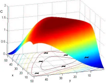
Fig.21shows that a constant capacity can be achieved in the interested
area, inside the projected internal circle, where the contributions of the six beams allow an extremely uniform QoS; besides, out of the service region the capacity obviously decreases since there are no
2.6 link budget analysis 27
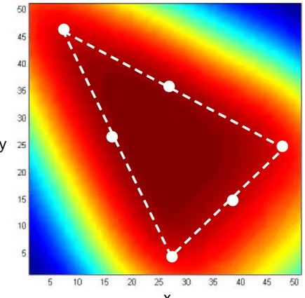
beams covering this area. This capacity shaping is clearly detailed also in Fig.22. The proposed strategy is easily scalable to a wider service
area with several beams which provide a very flat capacity all over it.
y
x
Figure 22: Snapshot of the capacity obtained in an area covered with six beams.
2.6 l i n k b u d g e t a na ly s i s
In the following a link budget analysis is shown for theSFSNconcept considering, for comparison, also the single beam case with a single carrier transmission and the single beam with OFDM. Note that the analysis has been conducted for a service in Kuband (carrier frequency
equal to 12GHz), but the same evaluation can be carried out for other bands. Moreover, aGEOsatellite is assumed.
All the systems have been dimensioned taking into account the best achievable coverage for an area of 650.000 km2 with the same total transmit power. In particular, for the single beam case, the effective antenna diameter of the satellite has been set to obtain the 3dB edge loss on the border of the coverage area. On the other hand, the effective antenna diameter of each beam in theSFSNhas been choose according to the considered beam geometry. In any case, in both the systems, all the parameters in Table1have been set in order to have the best trade-off
between coverage and link budget requirements. Results in Table 1
show that different signal to noise ratios (P/N) are experienced by a receiver using the three systems. In particular, the use ofOFDMboth in theSFSNconcept and in the single beam requires a larger Output Back Off (OBO) with respect to the single carrier approach. On the other hand, the combining of the signals coming from different beams, foreseen by theSFSNconcept, can compensate the losses in the link budget. In the
28 s i n g l e f r e q u e n c y s at e l l i t e n e t w o r k s
Table 1: Link budget for Single Beam andSFSNsystems.
Single Beam OFDM SFSN
Satellite Tsys 723K 723K 723K
Satellite Antenna Efficiency 0.65 0.65 0.65
Satellite Antenna Diameter 1m 1m 16m
Satellite Antenna Gain 40.11dBi 40.11dBi 64.20dBi
Satellite OBO 1dB 4dB 4dB
Satellite Input Loss 2dB 2dB 2dB
Satellite G/T 11.37dB/K 11.37dB/K 35.45dB/K
Receiver Tsys 150K 150K 150K
Receiver Antenna Efficiency 0.65 0.65 0.65
Receiver Antenna Diameter 0.9m 0.9m 0.9m
Receiver Antenna Gain 39.20dB 39.20dB 39.20dB Receiver G/T 17.44dB/K 17.44dB/K 17.44dB/K
Clear Air Atmospheric Loss 3dB 3dB 3dB
Frequency 12GHz 12GHz 12GHz
Bandwidth 500MHz 500MHz 500MHz
Path Loss 205.10dB 205.10dB 205.10dB
Number of Beams 1 1 400
Transmit Power per Beam 19.54dB 19.54dB −6.48dB Total Transmit Power 19.54dBW 19.54dBW 19.54dBW
EIRP 53.66dB 50.66dB 48.72dB
2.7 numerical evaluation 29
following section, a more complete comparison of the two systems is conducted, using the signal to noise ratios obtained in this analysis.
2.7 n u m e r i c a l e va l uat i o n
Now we calculate the capacity obtained with the single beam scheme and with theSFSNapproach. A vast service area of about 650.000 km2
has been considered. Note that this value approximately corresponds to a linguistic beam coverage region. The following assumptions have been used for theSFSNsystem:
• Service area covered with 400 beams organized in a uniform grid (20 × 20)
• NFFT = 2048
• Uniform spaced delays, δi= i⋅ δ0
• Number of multiple paths on each beam Ni equal to 3
• Uniform amplitude delay profile Ai= Awithin the same beam
• Same amplitude delay profile among different beams, A1= A2=
... = Ai=... = A(400)
• Incommensurable delays
Note that the analysis has been carried out considering the outputs of Table1, thus P
N equal to 7.60dB in the single beam single carrier
case, 4.60dB in the single beam with OFDM, and 2.67dB in the SFSN. Moreover, the service area has been discretized into 90 × 90 hexagonal cells and the capacity has been evaluated in their centers. Finally, since the capacity behavior is insensitive with respect to the phases φk, as
shown in Section2.3.4for incommensurable delays, a set of random φk
has been chosen for the sake of simplicity. Fig.23shows the capacity
comparison between the systems according to the link budget shown in Table1. As expected, a quasi-constant capacity can be achieved in the
interested area, where the contributions of the beams allow an uniform QoS; besides, out of the service region the capacity obviously decreases since there are no beams covering this area. On the other hand, the single beam single carrier approach outperformsSFSNin the zone closer to the center of the coverage area, but results in poorer performance in the zone around the boarder, while the single beamOFDMscheme presents the worst behavior. Note that the proposed strategy is easily scalable also to a smaller or a wider service area, just taking into account the beams position andMBCDDparameters.
2.8 s f s n: pros and cons
Let us dwell over the advantages and disadvantages of this approach. As for the main positive aspects, we consider the possibility to: use the same antenna pattern to provide broadcasting and broadband access, for triple play services; deliver efficiently local content and reuse that part of the spectrum extensively; shape precisely and adaptively the contour of beams by grouping spots; use power control selectively over those narrow beams where atmospheric conditions are bad; use a large number of smallHPAsinstead of a few powerfulHPAsfor the same total