Probabilistic approaches to recommendations

(1)

U

NIVERSITÀ DELLA

C

ALABRIA

Dipartimento di Elettronica,

Informatica e Sistemistica

Dottorato di Ricerca in

Ingegneria dei Sistemi e Informatica

XXVciclo

Tesi di Dottorato

Probabilistic Approaches to

Recommendations

Nicola Barbieri

D.E.I.S., Novembre 2012

(2)

(3)

DEIS- DIPARTIMENTO DI ELETTRONICA,INFORMATICA E SISTEMISTICA

Novembre

(4)

Preface

The design of accurate recommender systems is rapidly becoming one of the most successful application of data mining and machine learning techniques. Recommendation is a special form of information filtering, which extends the traditional concept of search, by modeling and understanding personal users’s preference. The importance of an accurate Recommender System is widely witnessed by both academic and industrial e↵orts in the last two decades. In this thesis, we are going to present and discuss the application of novel prob-abilistic approaches for the modeling of users’ preference data. We start our treatment by formally introducing the recommendation problem and sum-marizing the state of the art techniques for the generation of personalized recommendations. This analysis proves the e↵ectiveness of probabilistic mod-els based on latent factors in modeling and identifying patterns within the high dimensional (and exceptionally sparse) preference data. The probabilis-tic framework provides a powerful tool for the analysis and characterization of users and items, as it allows the identification of similar users and items which can be gathered in user communities and item categories.

Rooted on these backgrounds, our work focuses then on the problem of ef-fectively adopting probabilistic models to preference data. Our contributions can be summarized in three directions. First, we study the e↵ectiveness of the probabilistic techniques in generating accurate and personalized recom-mendation lists. Probabilistic techniques provide several kind of item ranking function which can be used to produce the recommendation list. This rankings focus on the estimate of the item selection, or on the predicted preference of each pair user,item or on a combination of these two, that we named item selection and relevance. The latter, which is based on the idea of predicting the chances that a user will “play and enjoy” a given content, is the best per-former in terms of recommendation accuracy, and we design two probabilistic methods for the direct estimation of this function from data. Finally, starting from the observation that thes high dimensional preference data may exhibit both global and local patterns, we propose and a probabilistic hierarchical model, in which user communities and item categories depend on each other.

(5)

VI Preface

This means that di↵erent user communities can exhibit di↵erent preference patterns on di↵erent item categories, where the identification of the latter depend on the considered community. This approach better models relation-ships between users and items and improve existing techniques both in terms of prediction and recommendation accuracy.

During the development of this thesis, it has been my privilege to work with brilliant and wonderful people. Among all, my sincere thanks go to Giuseppe Manco, for his support and guidance over the past three years. I am grateful for his collaboration whose benefits go over and above the learning of data mining techniques. His wide perspective, motivation, passion and, above all, his work ethical standards, had a great impact in shaping my enthusiasm towards research.

Rende,

(6)

1

(9)

2 1 The Recommendation Process

1.1 Introduction

With the increasing volume of information, products, services (or, more gen-erally, items) available on the Web, the role of Recommender Systems (RS) [1] and the importance of highly-accurate recommendation techniques have become a major concern both in e-commerce and academic research. In par-ticular, the goal of a RS is to provide users with not trivial recommendations, that are useful to directly experience potentially interesting items. Moreover, their exploitation in e-commerce can also provide more interactions between the users and the system, that can be profitably exploited for delivering more accurate recommendations. RSs are widely employed in di↵erent contexts, from music (Last.fm 1_{) to books (Amazon} 2_{), movies (Netflix} 3 _{) and news}

(Google News4_{[2] ), and they are quickly changing and reinventing the world}

of e-commerces[3].

Recommendation can be considered as a “push” system which provides users with a personalized exploration of a wide catalog of possible choices. While in a search based system the user is explicitly required to type a query (what she is looking for), here the query is implicit and corresponds to all the past interactions of the user with the system (items/web pages previ-ously purchased/viewed). Recommendations, as introduced before, help users in exploring and finding interesting items which the user may not found on her own. By collecting and analyzing past users’ preferences in the form of ex-plicit ratings or like/dislike products, the RSs provide the user with smart and personalized suggestions, typically in the form of “Customers who bought this item also bought” or “ Customers Who Bought Items in Your Recent History Also Bought”. The goal of the provider of the service is not just to trans-form a regular user in a buyer, but also make her browsing experience more confortable, building a strong loyalty bond . This idea is better explained by Je↵ Bezos (chief of Amazon.com) words: “If I have 3 million customers on the Web, I should have 3 million stores on the Web”.

The strategical importance of the development of always more accurate recommendation techniques has motivated both academic and industrial re-search for over 15 years; this is witnessed by huge investments in the devel-opment of personalized and high accuracy recommendation approaches. On October 2006, Netflix, leader in the movie-rental American market, released a dataset containing more of 100 million ratings and promoted a competition, the Netflix Prize 5[4], whose goal was to produce a 10% improvement on the prediction quality achieved by its own recommender system, Cinematch. The competition lasted three years and was attended by several research groups from all over the world, improving and inspiring a fruitful research. During

1 _last.fm 2 _amazon.com 3 _netflix.com 4 _{news.google.com} 5 _{netflixprize.com/}

(10)

1.2 Formal Framework 3

this period a huge number of recommendation approaches has been proposed and the improvements reached in personalization and recommendation en-couraged the emergence of new business models based on RSs.

In this chapter we will provide an overview of the recommendation sce-nario; in particular, we will firstly provide a formal framework which specifies some notations used throughout this work and discuss how to evaluate recom-mendations. Then we will introduce and discuss the most known collaborative filtering approaches, and we will present an empirical comparison of the main techniques.

1.2 Formal Framework

Recommendation is a particular form of information filtering which analyze past user’s preference on a catalog of items to generate a personalized list of suggested items. Thus, in the following, we will introduce some basilar notations to model users, items, and their associated preferences.

Let_{U = {u}1, . . . , uM} be a set of M users and I = {i1, . . . , iN} a set of N

items. For notational convenience, in the following, we reserve letters u, v to denote users from_{U and letters i, j to indicate items from I. User’ s} prefer-ences can be represented as a M_{⇥N matrix R, whose generic entry r}u

i denotes

the preference value (i.e., the degree of preference) assigned by user u to item i. User preference data can be classified as implicit or explicit. Implicit data corresponds to mere observations of co-occurrences of users and items. Hence, the generic entry ru

i of the user-item rating matrix R is a binary value.

Pre-cisely, ru

i = 0 means that u has not yet experienced i, whereas rui = 1 simply

signifies that user u has been observed to experience item i. Explicit data is more informative, since it records the actual ratings from the individual users on the experienced items. Ratings are essentially judgments on the interest-ingness of the corresponding items. Generally, in the context of real-world recommender systems, ratings are scores in a (totally-ordered) numeric do-main V, which is a fixed rating scale that often includes a small number of interestingness levels, such as a five-star rating scale. In such cases, for each pair_{hu, ii, rating values r}u

i fall within a limited rangeV = {0, . . . , V }, where

0 represents an unknown rating and V is the maximum degree of preference. Notation rR denotes the average rating among all those ratings rui > 0.

The number of users M as well as the number of items N are very large (typically with M >> N ) and, in practical applications, the rating matrix R is characterized by an an exceptional sparseness (e.g., more than 95%), since the individual users tend to rate a limited number of items. The set of items rated by user u is denoted by _IR(u) ={i 2 I|rui > 0}. Dually, UR(i) ={u 2

U|ru

i > 0} is the set of all those users, who rated item i. Any user u with

a rating history, i.e., such that IR(u)6= ; is said to be an active user. Both

IR(u) and UR(i) can be empty. This is known as cold start, and it generally

(11)

system. Cold start is generally problematic in recommender systems, since these cannot provide suggestions for users or items in the absence of sufficient information.

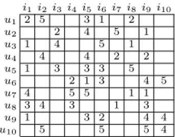
Fig 1.1 exemplifies the aforementioned notions. The illustration sketches a recommendation scenario with 10 users, 10 items and explicit observed pref-erences. The set of users who rated item i2isUR(i2) ={u1, u4, u8, u10}. Also,

the set of items rated by user u2isIR(u2) ={i3, i5, i7, i9}. The rating value of

user u2over item i4as well as the ratings from u4over i1and i3are unknown.

i1i2 i3i4i5i6i7 i8i9 i10 u1 2 5 3 1 2 u2 2 4 5 1 u3 1 4 5 1 u4 4 4 2 2 u5 1 3 3 3 5 u6 2 1 3 4 5 u7 4 5 5 1 1 u8 3 4 3 1 3 u9 1 3 2 4 4 u10 5 5 5 4

Fig. 1.1. Example of Rating Matrix.

Given an active user u, the goal of a RS is to provide u with a recom-mendation list _{L ✓ I including unexperienced items (i.e., L \ I}R(u) = ;),

that are expected to be of interest to u. This clearly involves predicting the interest of u into unrated items. Let ˆru

i denote the predicted rating of the user

u on the item i, while we denote by pu

i the overall predicted preference for the

same pair, which is actually used to produce a ranked list of items. In a first instance, we can assume that candidate items for recommendation are ranked according to their predicted preference. This assumption and other ranking functions will be later analyzed in Chap. 4.

1.2.1 Evaluation Metrics

Di↵erent evaluation metrics have been proposed in order to evaluate the ac-curacy of a RS[5, 6, 7]. Recommendations usually come in the form of a list of the k items that the user might like the most. Intuitively, an accuracy metric should measure how close the predicted list is to the actual ranked list of preferences of the user, or how close is the predicted rating from the its actual preference value. According to [5], evaluation metrics for recommendations can be classified in three classes: prediction accuracy, classification accuracy and rank accuracy metrics. Predictive accuracy metrics measure how close the predicted ratings are to the actual ratings. Classification accuracy is appro-priate metric in case of binary preferences, because it measures the frequency with which the system makes the right choice in the item suggestion phase. Rank accuracy metrics measure how close the top-k list of recommended items is close to the actual order of the same items.

(12)

1.2 Formal Framework 5

A common framework in the evaluation of the predictive capabilities of a RS algorithm is to split the rating matrix R into two matrices T and S, such that the former is used to train a recommendation algorithm, while the latter is used for validation purposes.

Prediction accuracy is measured by using statistical metrics that compare predicted values with actual ratings:

• Mean Absolute Error (MAE): measures the average absolute deviation between a predicted and a real rating. It is an intuitive metric, easily to compute and widely used in experimental studies:

M AE = 1 |S|

X

(u,i)2 S

|riu rˆui| . (1.1)

• Mean Squared Error (MSE): computes the mean squared error be-tween the observed ratings and the predicted values:

M SE = 1 |S| X (u,i)2 S (ru i rˆui) 2 . (1.2)

• Root Mean Squared Error (RMSE): it has been used as Netflix Prize metric for the prediction error. It is very similar to MSE but emphasizes large errors: RM SE = v u u t 1 |S| X (u,i)2 S (ru i ˆrui) 2 . (1.3)

• Mean Prediction Error (MPE): measures how many predictions di↵er from the actual rating values:

M P E = 1 |S|

X

(u,i)2 S

[rui 6= ˆrui] . (1.4)

MPE represents the percentage of data instances for which the recommen-dation system is not able to compute the exact observed rating.

Classification metrics measure the ability of the RS in detecting relevant items for each user. The recommendation list_Lufor the user u is generated by

ranking a set of candidate items according to a personalized ranking function. The accuracy of _Lu is ultimately assessed through a comparison with the

items appearing in_IS(u). Therein, the standard classification-based metrics,

i.e., precision and recall, can be adopted to evaluate the recommendation accuracy of the recommendation list. Such metrics require the capability to distinguish between relevant and irrelevant recommendations. Given a user u and a subset_Tr

u ✓ IS(u) of relevant items, the degree of precision and recall

(13)

Item relevance can be measured in several di↵erent ways. When explicit pref-erence values are available, we consider as relevant all those items that received a rating greater than the average ratings in the training set:

Tur={i 2 IS(u)|riu> rT}.

Precision and Recall are conflicting measures of the accuracy: for instance, by increasing the size of the recommendation list, Recall is expected to increase but Precision decreases. F-score is the harmonic mean of Precision and Recall, used to evaluate them in conjunction:

F = 2_· P recision· Recall

P recision + Recall. (1.6)

Finally, ranking accuracy metrics measure the ability of the RS to gener-ate a personalized ordering of the items, which match up with the the true users’ ordering. Typically the predicted and observed orderings are comparaed by using Kendall’s tau and Spearman’s rho.This perspective is without any doubts approach is the lack of data, since generally the full user-based ranking of all items is not available.

Evaluating recommendation is one of the biggest unsolved problem of cur-rent research in RSs. In particular:

• O✏ine evaluation rarely match up to online results;

• O✏ine metrics like Prediction/Recall, RMSE and MAP are poor proxies for what happens in the online world and they have been reported to be far from measuring the real impact of recommendations on users’ purchasing activities;

• Common evaluations do not consider the real users’s satisfaction.

In general, a more e↵ective evaluation should focus on how the user perceives recommendations and on measuring their helpfulness. Current research is in-vestigating several aspects correlated with evaluation, such as the analysis of the return of investment (ROI) in improving prediction and recommendation metrics and the proposal of more convincing o✏ine evaluation metrics.

1.3 Collaborative Filtering Approaches to

Recommendation

State-of-the art recommendation methods have been largely approached from a Collaborative Filtering (CF) perspective, which essentially consists in the

(14)

1.3 Collaborative Filtering 7

posterior analysis of past interactions between users and items, aimed to iden-tify suitable preference patterns in users’ preference data. Tapestry [8] is con-sidered the ancestor of CF systems. It was designed to support both content-based and collaborative filtering. Recording the reactions of each user on a particular document and explicit feedback, Tapestry allows mail filtering in an area of interest basing on other people annotations.

Modern CF techniques aim to predict the preferences values of users on given items, based on previously observed behavior. The assumption is that users who adopted the same behavior in the past, will tend to agree also in the future. The main advantage in using CF techniques relies on their simplicity: only users’ past ratings are used in the learning process, no further informa-tions, like demographic data or item descripinforma-tions, are needed. CF solves some of the main drawbacks of Content Based (CB) approaches [9, 10]:

• CF approaches are more general and re-usable in di↵erent context, while CB techniques require the specification of a complete profile (set of fea-tures) for each user/item;

• CB techniques provide the user with a list of products whose features are “similar” to ones that she experienced in the past. This approach may imply the recommendations of redundant items and the lack of novelty; • The e↵ectiveness of recommendation increases as the user provides more

feedback.

According to [11], collaborative filtering approaches can be classified in two classes, Memory-based and Model-based. The first class infers the preference of the active user on an item by using the database of preferences. The most common memory-based approaches are the Nearest Neighbors methods, which use the whole preference history of users and items and statistical techniques to infer similarities and then use this similarity measures to make a predic-tion. Model-based approaches operate in two phases: initially the preference database is used to learn a compact model and, in the second phase, this model is used in order to infer users’ preferences. Actually, memory-based approaches can rely on a model as well (i.e. similarity matrix in neighbors models), which is usually built in a o↵-line mode, but they still need to access to a database of preference values. Memory-based approaches are intuitive because, in the sim-plest case, they directly transforms stored preferences data in predictions, but they need to keep the whole dataset in memory. On the other hand, model-based approaches require less memory because they need to access only to the small-size model previously computed from the dataset, but the reason behind the provided predictions may not be easily interpretable. Moreover, memory-based approaches, such as Neighborhood models, are most e↵ective at detecting strong but local relationships, while model-based approaches, such as Latent Factor models, can estimate weak but global relationships. Figure 1.2 summarizes the di↵erent approaches used by the two methods.

(15)

!"#$%&'"()*+

',-.)/01"2,3& !,4.--,$3,)&

5/2(,- 6*7,89*2:*7,

9"("&'.3,: !,4.--,$3,)&'.3,:01"2,3&

5/2(,-6*7,89*2:*7, ;2 ,)2 <(,-2 = >

Fig. 1.2. Memory-based vs Model-based Approaches

In the following we will briefly review three family of CF approaches, namely Baseline, Nearest Neighbors and Latent Factor models, before focusing in more detail on Probabilistic Approaches in the next chapter.

1.3.1 Baseline Models

Baseline algorithms are the simplest approaches for predicting users’ numer-ical preferences. This section will focus on the analysis of the following al-gorithms: OverallMean, MovieAvg, UserAvg, DoubleCentering and the Global E↵ects Model.

OverallMean computes the mean of all ratings in the training set, this value is returned as prediction for each pair hu, ii. MovieAvg predicts the rating of a pairhu, ii as the mean of all ratings received by i in the training set. Similarly, UserAvg predicts the rating of a pairhu, ii as the mean of all ratings given by u. Given a pair hu, ii, DoubleCentering compute separately the mean of the ratings of the movie ¯ri, and the mean of all the ratings given by the user ¯ru.

The prediction is computed as a linear combination: ˆ

rui = ↵ ¯ri+ (1 ↵) ¯ru, (1.7)

where 0 ↵  1.

The Global E↵ects Model is considered one of the most useful and e↵ective technique in the context of the Netflix Prize. The key idea, proposed by Bell and Koren in [12] and widely appreciated by the Netflix Prize’s contestants, is to precede standard collaborative filtering algorithms with simple models that identify systematic tendencies in rating data, called global e↵ects. For example, some users might tend to assign higher or lower ratings to items respect to their rating average (user e↵ect), while some items tend to receive higher rating values than others (item e↵ect). Some other interesting consid-erations involve the time dimension: for example could be identified temporal patterns in user’s ratings which might rise or fall over period of time. A similar analysis could be performed on items: for example some movies might receive higher ratings when they first are proposed, while ratings might fall after their release period. The proposed strategy is to estimate and remove one global

(16)

e↵ect at time, in sequence: at each step we do not focus on the raw ratings but on the residuals of the previous step. In [12] authors identify 11 kind of e↵ects, and empirically evaluate the e↵ectiveness of this method by recording an improvement in RMSE after each cleaning step.

The main advantage of this approach relies on its capacity of removing noise from data. As instance, once global e↵ects has been completely removed from data, the K-Nearest Neighbors approach, which works better on residuals because they make possible to correctly identify neighbors and the actual strength of their relationships, could be used to compute the predicted resid-uals and then, the final predicted values could be obtained by adding the global e↵ects back.

1.3.2 Neighborhood-Based Approaches

Neighborhood based approaches [13, 14] compute each rating prediction by relying on a chosen portion of the data. According to a user-based perspective, the predicted rating on an item is generated by selecting the most similar users to the active one, said neighbors, and then using an aggregate function of their ratings. This intuitive definition corresponds to the classic behavior of asking friends for their opinions before purchasing a new item and it raises some fundamental questions:

1. How is it possible to model similarity about users/items? 2. How can we identify a neighborhood for the current user/item? 3. How can ratings of neighbors be used to generate a rating prediction? The most common formulation of the neighborhood approach is the K-Nearest-Neighbors (K-NN). The rating prediction ˆru

i is computed following

simple steps: (i) a similarity function associates a numerical coefficient to each pair of users, then K-NN finds the neighborhood of u by selecting her the K most similar users; (ii) the rating prediction is computed as the average of the ratings given by neighbors on the same item, weighted by the similarity coeffi-cients. The user-based K-NN algorithm is intuitive but doesn’t scale because it requires the computation of similarity coefficients for each pair of users. Considering that the number of items is generally lower than the number of users, a more scalable formulation can be obtained considering an item-based approach [13]. Thus, in the rest of the section, we will focus on item-based approaches. According to this perspective, the predicted rating for the pair hu, ii can be computed by aggregating the ratings given by u on the K most similar movies to i. The underlying assumption is that the user might prefer movies more similar to the ones he liked before, because they share similar features. The prediction is computed as:

ˆ riu= P j2N (i;u)si,j· ruj P j2NK_(i;u)si,j , (1.8)

(17)

where si,jis the similarity coefficient between i and j, andNK(i; u) is the set

of the K items evaluated by u which are most similar to i.

Similarity coefficients play a central role in the Neighborhood based ap-proaches: in the first phase they are used to identify the neighbors, while in the prediction phase they act as weights. Di↵erent techniques may be used to compute similarity coefficients for items or users and in most cases the similarity is computed by considering only the co-rated pairs. As instance, considering the case of the item-to-item similarity computation, only ratings from users who rated both the items are taken into analysis, Dually, the user-to-user similarity computation is commonly based on the ratings given on co-rated items. Let _UR(i, j) denote the set of users who provided a rating

for both i and j, i.eUR(i, j) =UR(i)\ UR(j). Similarity coefficients are often

computed according to the Pearson Correlation or the Adjusted Cosine, which improves the cosine similarity by taking into account the di↵erences in rating scale between di↵erent users[13]:

sij = P earson(i, j) = P u2UR(i,j)(r u i ri)· ruj rj qP u2UR(i,j)(r u i ri)2qPu2UR(i,j) r u j rj 2; sij = AdjCosine(i, j) = P u2UR(i,j)(r u i ru)· rju ru qP u2UR(i,j)(r u i ru)2qPu2UR(i,j) r u j ru 2.

As discussed in [15], similarity coefficients based on a larger support are more reliable than the ones computed using few rating values, so it is a com-mon practice to weight the similarity coefficients using the support size. This technique is called shrinkage:

s0i,j =

si,j· |UR(i, j)|

|UR(i, j)| + ↵

, (1.9)

where ↵ is an empirical value.

An improved version of K-NN can be obtained by refining the neighborhood model with baseline values. Formally:

ˆ rui = bui + P j2NK_(i;u)si,j· (ruj buj) P j2NK_(i;u)si,j , (1.10) where bu

i denote a baseline value.

An alternative way to estimate item-to-item interpolation weights is by solving a least squares problem minimizing the error of the prediction rule. This strategy, proposed in [16, 17], defines the Neighborhood Relationship Model, one of the most e↵ective approaches applied in the Netflix prize com-petition. In this case the prediction is computed as:

ˆ riu= P j2NK_(i;u)wi,j· rju P j2NK_(i;u)wi,j , (1.11)

(18)

where the non-negative interpolation weights wi,jare computed as the solution

of the following optimization problem: min W X v2UR(i) rvi P j2N (i;u,v)wi,j· rvj P j2N (i;u,v)wi,j !2 s.t. wi,j 08i, j 2 I

where the set_{N (i; u, v) is defined by all the items most similar to i which are} evaluated both by u and v.

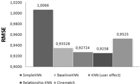
Fig. 1.3 shows the performance in prediction accuracy of K-NN mod-els. We empirically compare two di↵erent choices for the baseline function:

Fig. 1.3. Prediction Accuracy: K-NN models

BaselineK-NN relies on a double-centering baseline, whereas the K-NN (user e↵ect) version computes the baseline values according to the User E↵ect Model [12]. Except the SimpleK-NN, all the considered K-NN approaches improve Cinematch’s precision, and the best performance is achieved by the Neighbor-hood Relationship Model.

1.3.3 Latent Factor Modes

The assumption behind Latent Factor models is that the preference of the user can be expressed considering a set of contributes which represent and weight the interaction between her tastes and the target item on a set of features.

This approach has been widely adopted in information retrieval. For ex-ample, the Latent Semantic Indexing (LSI) [18] is a dimensionality reduction technique which assumes a latent structure in word usage across documents. LSI uses Singular Value Decomposition to represents terms and documents in the features space: some of these feature components are be very small and may be ignored, obtaining an approximate model. Given a m_{⇥ n matrix} A with rank r, the singular value decomposition of A, denoted by SV D(A) Figure 1.4, is defined as:

SV D(A) = U⇥ ⌃ ⇥ VT_, _(1.12)

(19)

• U is an m ⇥ m orthogonal matrix6_{; the first r columns of U are the}

eigenvectors of AAT (left singular vectors of A);

• V is an n ⇥ n orthogonal matrix; the first r columns of V are the eigen-vectors of AT_{A (right singular vectors of A);}

• ⌃ is a n ⇥ n diagonal matrix with only r nonzero values, such that: ⌃ = { 1,· · · , n} , i 08 1  i < n, i i+1, j= 08 j r + 1;

• { 1,· · · , n} are the nonnegative square root of the eigenvalues of ATA

and are called singular values of A.

Fig. 1.4. Singular Value Decomposition

SVD has an important property: it provides the best low-rank linear approx-imation of the original matrix A. Fixed a number k _{ r, called dimension} of the decomposition, the matrix Ak =Pki=1ui iviT minimizes the Frobenius

norm _kA AkkF over all rank-k matrices. Therefore, focusing only on the

first k singular values of ⌃ and reducing the matrices U and V, the original matrix can be approximated using Ak:

A⇡ Ak= Uk⌃kVTk (1.13)

where Uk is obtained by removing (r k) columns from the matrix U and

VT

k is produced by removing (r k) rows from the matrix V . An example of

this approximation is given in Figure 1.5. Considering the text analysis case, LSI factorizes the original term-document matrix into the product of three matrices which reflects the relationships between each single term and docu-ment in the k features-space, where k is the number of considered features. The derived matrix Ak is not the exact factorization of A: the procedure of

selecting only the k largest single values captures the underlying structure of A, removing at the same time noise [19].

Several works have studied the application of SVD in recommender systems [20, 21]: the dimensional reduction approach is very useful for CF because is able to produce a low-dimensional representation of the original high-dimensional rating matrix R and to capture the hidden relationships between

(20)

Fig. 1.5. k-rank approximation of A

users and products that could be used to infer the user’s preference on consid-ered items. Focusing on a scenario that involves ratings given by a set of users on a set of movies, it is plausible to assume that the user’s rating on a movie is influenced by a set of feature of the movie itself and by the user’s prefer-ence on those feautures. An intuitive idea of what of hidden features might represent in this scenario, is the genre interpretation: assuming the existence of a limited number of di↵erent genres of movies (action, romance, comedy, etc.), the rating is influenced by the user’s preference on those genres and by a movie’s factors that represent how much the considered movie belongs to each genre. Figure 1.6 shows an example of this scenario, with 3 hidden factors.

Fig. 1.6. Example of the application of SVD decomposition

With an abuse of notation, in this section will use a simplified but equiva-lent formalization for the SVD, in which the original matrix is approximated by the product of 2 component matrices with K features:

R_⇡⇣Uk p ⌃Tk ⌘ ⇣p ⌃kVTk ⌘ = U_{· V,} (1.14)

where U is a M ⇥ K matrix and V is a K ⇥ N. Intuitively, each users’s preference on an item matrix is decomposed as the product of the dimensional projection of the users and items into the K-dimensional feature space:

ˆ ru i = K X k=1 Uu,k· Vk,i. (1.15)

(21)

Fixed the number of features K, we can estimate the feature matrices by solving this optimization problem:

(U, V) = arg min

U,V 2 4 X (u,i)2 T rui K X k=1 Uu,kVk,i !3 5 . (1.16)

Funk in [22] proposed an incremental procedure, based on gradient descent, to minimize the error of the model on observed ratings. The feature matrices are randomly initialized and updated as follows:

U0u,k= Uu,k+ ⌘ (2eu,i· Vk,i) ,

V0k,i= Vk,i+ ⌘ (2eu,i· Uu,k) ,

(1.17) where eu,i= ˆrui riuis the prediction error on the pairhu, ii and ⌘ is the

learn-ing rate. The optimization procedure could be further improved considerlearn-ing regularization coefficients . Updating rules become:

U0u,k= Uu,k+ ⌘ (2eu,i· Vk,i · Uu,i) ,

V0k,i= Vk,i+ ⌘ 2eu,i· U0u,k · Vk,i .

(1.18) A more refined model can be obtained by integrating a combining a baseline model with the SVD prediction:

ˆ rui = bui + K X k=1 Uu,k· Vk,i, (1.19)

or considering user and item bias components [23]: ˆ rui = cu+ di+ K X k=1 Uu,k· Vk,i, (1.20)

where cu is the user-bias vector and di is the item-bias vector, which are

trained simultaneously with the features matrices with regularization rate 2:

c0u= cu+ ⌘ (eu,i 2(cu+ di r¯T))

d0i= di+ ⌘ (eu,i 2(cu+ di r¯T)) .

(1.21) An alternative and more e↵ective formulation, known as Asymmetric SVD [23], models each user by exploiting all the items that she rated:

Uu,k= p 1

|I(u)| + 1 X

i2 I(u)

wk,i. (1.22)

A slightly di↵erent version, named SVD++ [15], models each user by consid-ering both a user-features vector and the corresponding bag-of-items repre-sentation.

(22)

Latent factor models based on the SVD decomposition change according to the number of considered features and the structure of model, characterized by presence of bias and baseline contributes. The optimization procedure used in the learning phase plays an important role: learning could be incremental (one feature at the time) or in batch (all features are updated during the same iteration of data). Incremental learning usually achieves better performances at the cost of learning time.

To assest the predictive capabilities of latent factor models, we tested several version of SVD model, considering the batch learning with learning rate 0.001. The regularization coefficient, where needed, has been set to 0.02. To avoid overfitting, the training set has been partitioned into two di↵erent parts: the first one is used as actual training set, while the second one, called validation set, is used to evaluate the model. The learning procedure is stopped as soon the error on the validation set increases. Fig.1.7 shows the accuracy of the main SVD approaches. An interesting property of the analyzed models is that they reach convergence after almost the same number of iteration, no matter how many features are considered. Better performances are achieved if the model includes bias or baseline components; the regularization factors decrease the overall learning rate but are characterized by an high accuracy. In the worst case, the learning time for the regularized versions is about 60 min. The SVD++ model with 20 features obtains the best performance with a relative improvement on the Cinematch score of about 5%.

(a) (b)

(23)

(24)

2

(25)

18 2 Probabilistic Approaches to Preference Data

2.1 Introduction

Probabilistic approaches assume that each preference observation is randomly drawn from the joint distribution of the random variables which model users, items and preference values (if available). Typically, the random generation process follows a bag of words assumption and preference observations are as-sumed to be generated independently. A key di↵erence between probabilistic and deterministic models relies in the inference phase: while the latter ap-proaches try to minimize directly the error made by the model, probabilistic approaches do not focus on a particular error metric; parameters are deter-mined by maximizing the likelihood of the data, typically employing an Ex-pectation Maximization procedure. In addition, background knowledge can be explicitly modeled by means prior probabilities, thus allowing a direct control on overfitting within the inference procedure [24]. By modeling prior knowl-edge, they implicitly solve the need for regularization which a↵ects traditional gradient-descent based latent factors approaches.

Further advantages of probabilistic models can be found in their easy inter-pretability: they can often be represented by using a graphical model, which summarizes the intuition behind the model by underlying causal dependen-cies between users, items and hidden factors. Also, they provide an unified framework for combining collaborative and content features [25, 26, 27], to produce more accurate recommendations even in the case of new users/items. Moreover, assuming that an explicit preference value is available, probabilis-tic models can be used to model a distribution over rating values which can be used to infer confidence intervals and to determine the confidence of the model in providing a recommendation.

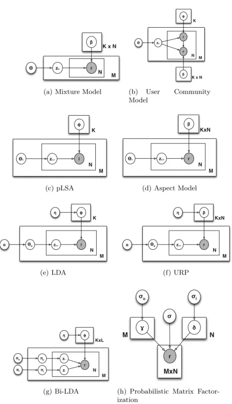
In the following we will briefly introduce some paradigmatic probabilistic approaches to recommendation, which can be categorized into 3 main classes: Mixture Models, Probabilistic Topic Models and Probabilistic Matrix Factor-ization Techniques. Fig. 2.1 o↵ers an overview of the generative models of the main techniques. The underlying idea of probabilistic models based on latent factors is that each preference observationhu, ii is generated by one of k possible states, which informally model the underlying reason why u has chosen/rated i. Based on the mathematical model, two di↵erent inferences can be then supported to be exploited inthe modelling of preference data [28]: • Forced Prediction: the model provides estimate of P (r|u, i), which repre-sents the conditional probability that user u assign a rating value r given the item i;

• Free prediction: the item selection process is included in the model, which is typically based on the estimate of P (r, i_{|u). In this case we are interested} in predicting both the item selection and the preference of the user for each selected item. P (r, i|u) can be factorized as P (r|i, u)P (i|u); the resulting model still includes a component of forced prediction which however is weighted by the item selection component and thus allows a more precise estimate of user’s preferences.

(26)

2.2 Mixture Models 19

2.2 Mixture Models

A mixture model [29] is a general probabilistic approach which introduces a set of latent factor variables to represent a generative process in which data points may be generated according to a finite set of probability distribution. The simplest latent factor approach to model users’ preference data is the Multinomial Mixture Model (MMM, [30]). According to this model, we assume that a user u is associated with a latent factor z, which models her “attitude”, and ratings for an item i are generated according to this factor. The corresponding generative semantic, represented graphically in Figure 2.1(a), can be summarized as:

1. For each user u =_{{1, · · · , M}}

a) Sample a user attitude z according to a multinomial distribution over the latent variable ✓

b) For each i2 I(u)

i. Draw a rating value r according to multinomial distribution over rating values i,z

The ✓ parameter here is the prior probability distribution over the possibile states of the latent variables, P (Z), whereas i,z is a multinomial overV which

drives for the rating generation P (R = r|i, z). The learning of the parameter of the model can be accomplished by employing the EM algorithm, which also provides, with the “responsibilities”, an estimate of the mixing proportion for each user P (z|u). Given those parameters, the probability distribution over ratings for the pairhu, ii can be computed as:

P (r_{|i, u) =} K X z=1 P (z_{|u) ·} z,i,r (2.1) where P (z|u) / P (uobs|z)✓z

and uobsrepresents the observed values (u, i, r) in R.

The User Communities Model (UCM, [31]) (see Sec. 5.2.1) refines the inference formula Eq. 2.1 by introducing some key features. First, the exploitation of a unique prior distribution ✓ over the user communities helps in preventing overfitting. Second, adds flexibility in the prediction by modeling an item as an observed (and hence randomly generated) component, thus following a free-prediction perspective.

(27)

20 2 Probabilistic Approaches to Preference Data β zu r K x N N Ɵ M

(a) Mixture Model

β zu r K x N N Ɵ M i φ K (b) User Community Model zu,n N Ɵu M i φ K (c) pLSA zu,n N Ɵu M r β KxN (d) Aspect Model zu,n N Ɵu M i φ K η α (e) LDA zu,n N Ɵu M r β KxN η α (f) URP zu N πu M r φ KxL η αu zi πi αi (g) Bi-LDA r MxN ɣ σ_u σ_i M ð σ N

(h) Probabilistic Matrix Factor-ization

(28)

2.3 Probabilistic Topic Models 21

2.3 Probabilistic Topic Models

Probabilistic Topic models [32, 33, 34] include a suite of techniques which widely used in text analysis: they provide a low-dimensional semantic repre-sentation that allows the discovering of global relationships within data. Given a corpus of documents, the assumption behind this family of techniques is that each document may exhibit multiple topics and each word in the document is generated by a particular topic. A generative process for CF, based on latent topics, is shown in Figure 2.2. In the CF context, topics could be interpreted as

Fig. 2.2. Latent Class Model for CF - Generative Process

genres, item categories or user’s attitudes, although no prior meaning is gen-erally associated with them. A proper definition of topics might be obtained by considering them as “abstract preference pattern”: users, or items, partic-ipate in each preference pattern with a certain degree, and these membership weights project each user/item into the latent factor space. We assume that there are a fixed number of topics, and each user is characterized by her own preference on genres. For example, in Figure 2.2, the considered user shows a particular interest in action and historic movies, while her interest in ro-mance is low. Each genres specifies the probability of observing each single item. Movies like “Independence Day” and “Die hard” will have an higher probability of being observed given the “action” topic, than in the context of “romance”. Given an user and her preferences on topics (which defines prefer-ences on movies), the corresponding purchasing history can be generated by choosing a topic, and then drawing an item from the corresponding distribu-tion over items. In the example, the first topic to be chosen is “acdistribu-tion”, which generates the movie “Die Hard”; the process of topic and item selection is iteratively repeated to generate the complete purchase history of the current user.

The probabilistic Latent Semantic Analysis approach (PLSA, [35, 36]) specifies a co-occurrence data model in which the user u and item i are conditionally independent given the state of the latent factor Z. Di↵erently from the previous mixture model, where a single latent factor is associated

(29)

with every user u, the PLSA model associates a latent variable with every observation triplethu, i, ri. Given an active user u, her purchase history can be generated according to the following generative semantic:

1. For n = 1 to|I(u)|:

a) Select a user profile z according to user-specific multinomial dis-tribution over topics ✓u= P (Z = z|u);

b) Pick an item i by sampling from the multinomial distribution

z= P (i|z);

Hence, di↵erent ratings of the same user can be explained by di↵erent latent causes in PLSA (modeled as priors_{✓u}1,...,min Figure 2.1(c)), whereas

a mixture model assumes that all ratings involving the same user are linked to the same underlying community. PLSA directly supports item selection:

P (i_{|u) =}

K

X

z=1

z,i✓u,z (2.2)

where zrepresents a multinomial distribution over items. The main drawback

of the PLSA approach is that it cannot directly model new users, because the parameters ✓u,z= P (z|u) are specified only for those users in the training set.

We consider three further variants for the PLSA, where explicit preferences are modeled by an underlying distribution z,i. In the Aspect Model (AM,

[36]) z,i is a multinomial overV. In this case, the rating probability can be

modeled as P (r|u, i) = K X z=1 r,i,z✓u,z (2.3)

Conversely, the Gaussian PLSA (G-PLSA, [24]) models z,i= (µiz, iz) as

a gaussian distribution, and provides a normalization of ratings through the user’s mean and variance, thus allowing to model users with di↵erent rating patterns. The corresponding rating probability is

P (r|u, i) =

K

X

z=1

N (r; µiz, iz)✓u,z (2.4)

The Flexible Mixture Model (FMM) [37] extends the Aspect Model, by allowing each user/item to belong to multiple clusters, which are deter-mined simultaneously, according to a coclustering approach. Assuming the existence of K user clusters indexed by c and L item clusters, indexed by d, and let P (ck) be the probability of observing the user-cluster k with P (u|ck)

(30)

2.3 Probabilistic Topic Models 23

using the same notations for the item-cluster, the joint probability P (u, i, r) is defined as: P (u, i, r) = C X c=1 D X d=1 P (c)P (d)P (u_{|c)P (i|d)P (r|c, d)}

The Latent Dirichlet Allocation [32] is designed to overcome the main drawback in the PLSA-based models, by introducing Dirichlet priors, which provide a full generative semantic at user level and avoid overfitting. The generative process that characterized LDA can be formalized as follows:

1. For each user u =_{{1, · · · , M}}

a) Choose Nu according to a Poisson’s distribution, or to any other

distribution that could model the number of items in the user profile

b) Choose ✓u⇠ Dir(↵)

c) For each of the Nu items to be generated:

i. Choose a topic z_{⇠ Multinomial(✓}u)

ii. Choose an item i according to the multinomial probability conditioned on the selected topic: P (i|z, )

Again, two di↵erent formulations, are available, based on whether we are interested in modeling implicit (LDA) or explicit (User Rating Profile, URP[38]) preference values. In the first case, we have:

P (i|u) = Z _XK

z=1

z,i✓zP (✓|uobs)d✓ (2.5)

(where P (✓_|uobs) is estimated in the inference phase). Analogously, for the

URP we have

P (r_{|u, i) =} Z _XK

z=1

z,i,r✓zP (✓|uobs)d✓ (2.6)

The idea behind the models presented so far, is the starting point of more advanced approaches that include side information to achieve better results in prediction accuracy and provide tools for cold-start recommendation [26, 25, 39]. Interesting results have been obtained by adopting a co-clustering structure [40, 41, 42, 37, 43]. As instance, the Bi-LDA model proposed in [43] (represented in Figure 2.1(g)), extends the URP model employing two interacting LDA models which enforce the simultaneous clustering of users and items in homogeneous groups. The rating probability according to this bayesian coclustering model can be computed as:

(31)

P (r_{|u, i) =}Z Z X

zu,zi

(2.7) where both P (⇡u|uobs) and P (⇡i|iobs) are estimated in the inference phase.

The generative process of the Bi-LDA is as follows:

1. For each user u =_{{1, · · · , M}}

a) Choose Nu according to a Poisson’s distribution

b) For each of the Nu items to be generated:

i. Choose a user attitude zu

u,n⇠ Discrete(⇡u)

ii. Choose an item category zi

u,n⇠ Discrete(⇡i)

iii. Generate a rating value for the chosen item according to the distribution P (r|'zu

u,n,ziu,n)

2.4 Probabilistic Matrix Factorization

The Probabilistic Matrix Factorization approach (PMF, [44]) reformu-lates the rating assignment as a matrix factorization. Given the latent user and item k-feature matrices u and i, (where K denotes the number of the

features employed in the factorization), the preference value is generated by assuming a Gaussian distribution over rating values conditioned on the inter-actions between the user and the considered item in the latent space, as shown in Figure 2.1(h). In practice, P (r|u, i) is modeled as a gaussian distribution, with mean T

u i and fixed variance :

P (r|u, i) = N (r; T

u i, 2) (2.8)

The conditional distribution of the observed data, given the latent user and item feature matrices, and , is computed as

P (R| , , ) = M Y u=1 N Y i=1 N (ru i; u iT , 2) (u, i)

where (u, i) is an indicator function that is equal to 1 if the user u has rated the item i, zero otherwise. Moreover, to avoid overfitting, user and item features are generated by two zero-mean spherical Gaussian priors:

P ( | u) = M Y u=1 N ( u; 0, 2uI) P ( | i) = N Y i=1 N ( i; 0, i2I)

Di↵erent extensions of the basic framework have been proposed: a constrained version [44] of the PMF model is based on the assumption that users who have

(32)

2.4 Probabilistic Matrix Factorization 25

rated similar sets of items are likely to exhibit similar preferences, while its bayesian generalizations [45] and extensions with side information [46, 47, 48] are characterized by an higher prediction accuracy.

(33)

(34)

3 Pattern Discovery and Users’ Profiling in CF

Data

(35)

28 3 Pattern Discovery and Users’ Profiling in CF Data

3.1 Introduction

Recent studies [49, 50] have shown that the focus on prediction does not necessarily helps in devising good recommender systems. As the number of available customers increases, is always more difficult to understand, profile and segment their behaviors and a similar consideration holds for the catalog of products. Under this perspective, CF models should be considered in a broader sense, for their capability to understand deeper and hidden relation-ships among users and products they like. For example, the high dimensional preference matrix can be partitioned to detect user communities and item categories; the analysis of the relationships between these two levels can pro-vide a faithful yet compact description of the data which can be exploited for better decision making.

The latent variable modeling, exploited within a probabilistic framework, of-fers some important, and easily interpretable, insights into the users’s pur-chase and preference patterns. In this chapter we are going to discuss some of the applications of probabilistic models to the task of pattern discovery in collaborative filtering data.

A first study which describes the application of probabilistic approaches, to understand users’s preference and interests, is presented in [51]. In this work, authors exploited the pLSA model to infer the underlying task of a web browsing session and to discover hidden semantic relationships between users and web pages. More specifically, the web session of the user u can be represented using co-occurrence pairs notations (u, p), where p is a collection of web objects, called pageview, resulting from a single action of the user. During a web session the user can visit di↵erent pageviews, and their corresponding importance within the session can be represented using a weight function w(u, p), which could be binary (existence or non existence of the pageview in a user session) or numeric (number of times that the pageview p is visited within the same user session, duration of the pageview in that session). The probability distributions that define the pLSA model and other probabilities, like the prior P (z) or the user specific distribution P (z|u), which can be obtained by marginalization or Baye’s rule, allow the following analysis: • Characterize Topics by Items: Each topic, represented by a latent

factor, can be characterized by a set of web pages which are strongly as-sociated with it. Those pages, or in general products belonging to an user purchase session, are called characteristic objects for the topic z. Intu-itively, a characteristic page given a topic z is a page which exhibits an high probability of being observed given the considered topic (P (i_{|z) is} high) and a low probability for being generated by other di↵erent top-ics. The characteristic objects for a topic zk can be defined as the set of

products/pages, indexed by i, such that: P (i|zk)· P (zk|i) µ, where µ

is a fixed threshold. Characteristic objects identification allows a better understanding of hidden factors. The pLSA model does not associate any a priori meaning with the states of the hidden variables which are used to

(36)

3.1 Introduction 29

detect relationships between users, grouping like-minded users in the same community, and items, grouping similar items in the same category. Char-acteristic objects might provide a posteriori interpretation for the state of the hidden variable, which can be an useful starting point for the following analysis of users patterns and relationships between di↵erent topics. • Characterize Topics by User Histories: A similar approach can be

used to associate each topic with a set of characteristic users. A charac-teristic user uk for a given topic zk is an user which prefers zk over the

other di↵erent topics, which implies that a wide fraction of the products in the purchase history of uk share the topic zk. The characteristic users

for the topic zk can be formally defined as the set of users u which

sat-isfy P (u|zk)· P (zk|u) µ. In this case p(u|zk) can be computed from

P (Z = z|u) by applying the Bayes’ rule.

• User Segments Identification: The relationships among the state of the hidden variable, users and items can be used to understand common inter-ests and preferences of users. An user segment is a set of users that shared a similar topic in their past sessions. The user segment corresponding to the topic zk can be computed by selecting those users with P (u|zk) µ

where the parameter µ is used as threshold. A projection of the user seg-ment into the item space can be obtained considering the most frequent items for the user segment.

• Topic Identification: the pLSA model provides an easy way to iden-tify the topic in a given user session. Given an active user u and a list of items/pages recently purchased/viewed called session, the probabil-ity P (z_{|session) can be estimated via a modified version EM algorithm,} known as folding-in approach [52], in which the the probabilities P (i_|z) are fixed.

In the next, we are going to discuss two novel applications of probabilistic approaches to pattern discovery in CF data. Mutual relationship between users and items can be detected by means of co-clustering approaches. The key idea is that similar users are detected by taking into account their ratings on similar items, which in turn are identified considering the ratings assigned by similar users. In Sec. 3.2, we will provide a co-clustering approach to model preference data, and then we will discuss some of its applications.

As the volume of the users grows, users profiling and segmentation techniques are becoming essential to understand their behavior and needs. Identifying groups of similar minded users is a powerful tool to develop targeted marketing campaigns. Motivated by these observations, in Sec. 3.3 we will propose a probabilistic method to detect communities of customers who exhibit the same preference patterns.

(37)

3.2 Characterizing Relationships Through Co-Clustering

In this section we present a co-clustering approach to preference prediction and rating discovery. Unlike traditional CF approaches, which try to discover similarities between users or items using clustering techniques or matrix de-composition methods, the aim of the BMM is to partition data into homo-geneous blocks enforcing a simultaneous clustering which consider both the dimension of the preference data. This approach highlights the mutual rela-tionship between users and items: similar users are detected by taking into account their ratings on similar items, which in turn are identified considering the ratings assigned by similar users.

To detect this hidden block structure within preference matrix, in the fol-lowing we will provide an extension the Block Mixture Model (BMM) proposed in [53, 54] for binary incidence matrices. We extend the original BMM formula-tion to model each preference observaformula-tion as the output of a gaussian mixture employing a maximum likelihood (ML) approach to estimate the parameter of the model. The strict interdependency between user and item cluster makes difficult the application of traditional optimization approaches like EM; thus, we perform approximated inference based on a variational approach and a two-step application of the EM algorithm. The block structure retrieved by the model in the inference phase allows to infer patterns and trends within each block. Overall, the proposed model guarantees a competitive prediction accuracy with regards to state-of-the art co-clustering approaches, it allows to infer topics for each item category, and finally allow as learn character-istic items for each user community, or to model community interests and transitions among topics of interests.

3.2.1 A Block Mixture Model for Preference Data

In this section, we are interested in devising how the available data fits into ad-hoc communities and groups, where groups can involve both users and items. Fig. 5.1 shows a toy example of preference data co-clustered into blocks. As we can see, a coclustering induces a natural ordering among rows and columns, and it defines blocks in the preference matrix with similar ratings. The discovery of such a structure is likely to induce information about the population, and to improve the personalized recommendations.

Formally, a block mixture model (BMM) can be defined by two partitions (z, w) which, in the case of preference data and considering known their re-spective dimensions, have the following characterizations:

• z = {z1,· · · , zK} is a partition of the user set U into K clusters and

zuk= 1 if u belongs to the cluster k, zero otherwise;

• w = {w1,· · · , wL} is a partition of the item set I into L clusters and

(38)

3.2 Characterizing Relationships Through Co-Clustering 31

Fig. 3.1. Example Co-Clustering for Preference Data

Given a rating matrix R, the goal is to determine such partitions and the respective partition functions which specify, for all pairshu, ii the probabilistic degrees of membership wrt. to each user and item cluster, in such a way to maximize the likelihood of the model given the observed data. According to the approach described [53, 54], and assuming that the rating value r observed for the pair_{hu, ii is independent from the user and item identities, fixed z and} w, the generative model can be described as follows:

1. For each u generate zu⇠ Discrete(⇡1; . . . ; ⇡K)

2. for each i generate wi⇠ Discrete( 1; . . . ; L)

3. for each pair hu, ii:

• detect k and l such that zuk= 1 and wil= 1

• generate r ⇠ N(R; µl

k, lk)

The corresponding data likelihood in the Block Mixture can be modeled as p(R, z, w) = Y u2U p(zu) Y i2I p(wi) Y hu,i,ri2R P (r_|zu, wi)

and consequently, the log-likelihood becomes: Lc(⇥; R, z, w) = K X k=1 X u2U zuklog ⇡k+ L X l=1 X i2I willog l + X hu,i,ri2R X k X l ⇥ zukwillog '(r; µlk, kl) ⇤ (3.1)

where ⇥ represents the whole set of parameters

⇡1, . . . , ⇡K, 1, . . . , L, µ11, . . . , µLK, 11, . . . , KL ,

and '(r; µ, ) is the gaussian density function on the rating value r with parameters µ and : '(r; µ; ) = (2⇡) 1/2 1_exp ✓ ₁ 2 2(r µ) 2 ◆

(39)

Inference and Parameter Estimation.

Denoting P (zuk = 1|u, ⇥(t)) = cuk, P (wil = 1|i, ⇥(t)) = dil and P (zukwil =

1_{|u, i, ⇥}(t)_{) = e}

ukil, The conditional expectation of the complete data

log-likelihood becomes: Q(⇥; ⇥(t)) = K X k=1 X u cuklog ⇡k+ L X l=1 X i dillog l+ X hu,i,ri2R X k X l ⇥ eukillog '(r; µlk, kl) ⇤

As pointed out in [53], the above function is not tractable analytically, due to the difficulties in determining eukil; nor the adoption of its variational

approx-imation (eukil = cuk · dil) allows us to derive an Expectation-Maximization

procedure for Q0_{(⇥, ⇥}(t)_{) where the M-step can be computed in closed form.}

In [53] the authors propose an optimization of the complete-data log-likelihood based on the CEM algorithm. We adapt the whole approach here. First of all, we consider that the joint probability of a a normal population xi with i = 1

to n can be factored as:

n Y i=1 '(xi; µ, ) = h(x1, . . . , xn)⇤ '(u0, u1, u2; µ, ), where h(x1, . . . , xn) = (2⇡) n/2, '(u0, u1, u2; µ, ) = u0exp ✓_2u 1µ u2 u0µ2 2 2 ◆ , and u0, u1 and u2 are the sufficient statistics.

Based on the above observation, we can define a two-way EM approxima-tion based on the following decomposiapproxima-tions of_Q0_:

Q0(⇥, ⇥(t)) =_Q0(⇥, ⇥(t)_{|d) +}X i2I L X l=1 dillog l X u2U X i2I(u) dil/2 log(2⇡) where Q0(⇥, ⇥(t) |d) = M X u=1 K X k=1 cuk(log(⇡k) + ⌧uk) ⌧uk = L X l=1

log⇣'(u(u,l)0 , u

(u,l) 1 , u (u,l) 2 ; µlk, lk) ⌘ u(u,l)₀ = X i2I(u) dil; u(u,l)1 = X i2I(u) dilriu; u (u,l) 2 = X i2I(u) dil(rui) 2

(40)

3.2 Characterizing Relationships Through Co-Clustering 33 Analogously, Q0(⇥, ⇥(t)) =_Q0(⇥, ⇥(t)_{|c) +}X u2U K X k=1 cuklog ⇡k X i2I X u2U(i) cuk/2 log(2⇡) where Q0(⇥, ⇥(t)|c) = N X i=1 L X l=1 dil(log( l) + ⌧il) ⌧il= K X k=1

log⇣'(u(i,k)₀ , u(i,k)₁ , u(i,k)₂ ; µlk, kl)

⌘ u(i,k)₀ = X u2I(u) cuk; u(i,k)1 = X u2I(u) cukrui u (i,k) 2 = X u2I(u) cuk(rui) 2

The advantage in the above formalization is that we can approach the single components separately and, moreover, for each component it is easier to estimate the parameters. In particular, we can obtain the following:

1. E-Step (user clusters): cuk= P (u_|zk)· ⇡k PK k0=1P (u|zk0)· ⇡k0 P (u_|zk) = L Y l=1 '(u(u,l)0 , u (u,l) 1 , u (u,l) 2 ; µlk, kl)

2. M-Step (user clusters): ⇡k= P u2Ucuk M µlk= PM u=1 P i2I(u)cukdilriu PM u=1 P i2I(u)cukdil ( kl)2= PM u=1 P i2I(u)cukdil(riu µlk)2 PM u=1 P i2I(u)cukdil

3. E-Step (item clusters): dil=P_LP (i|wl)· l l0=1p(i|wl0)· l0 P (i|wl) = K Y k=1 '(u(i,k)0 , u (i,k) 1 , u (i,k) 2 ; µlk, lk)

4. M-Step (item clusters):

l= P i2Idil N µlk= PN i=1 P u2U(i)dilcukrui PN i=1 P u2U(i)dilcuk ( lk)2= PN i=1 P u2U(i)cukdil(rui µlk)2 PN i=1 P u2U(i)dilcuk

(41)

Rating Prediction

The blocks resulting from a co-clustering can be directly used for prediction. Given a pair_{hu, ii, the probability of observing a rating value r associated to} the pair_{hu, ii can be computed according to one of the following schemes:} • Hard-Clustering Prediction: P (r_{|i, u) = '(r; µ}l k, lk), where k = argmax j=1,··· ,K cuj and l = argmax h=1,··· ,L dih are

the clusters that better represent the observed ratings for the considered user and item respectively.

• Soft-Clustering Prediction:

P (r_{|i, u) =} PK_k=1PL_l=1cukdil'(r; µlk, lk), which consists of a weighted

mixture over user and item clusters.

The final rating prediction can be computed by using the expected value of P (r_{|u, i).}

In order to test the predictive accuracy of the BMM we performed a suite of tests on a sample of Netflix data. The training set contains 5, 714, 427 ratings, given by 435, 656 users on a set of 2, 961 items (movies). Ratings on those items are within a range 1 to 5 (max preference value) and the sample is 99% sparse. The test set contains 3, 773, 781 ratings given by a subset of the users (389, 305) in the training set over the same set of items. Over 60% of the users have less than 10 ratings and the average number of evaluations given by users is 13.

We evaluated the performance achieved by the BMM considering both the Hard and the Soft prediction rules and performed a suite of experiments varying the number of user and item clusters. Experiments on the three models have been performed by retaining the 10% of the training (user,item,rating) triplets as held-out data and 10 attempts have been executed to determine the best initial configurations. Performance results measured using the RMSE for two BMM with 30 and 50 user clusters are showed in Figure 3.2(a) and Figure 3.2(b), respectively. In both cases the soft clustering prediction rule overcomes the hard one, and they show almost the same trend. The best result (0.9462) is achieved by employing 30 user clusters and 200 item clusters. We can notice from Table 3.1 that the results follow the same trend as other probabilistic models (pLSA[28], FMM [37], ScalableCC[55]).

Method Best RMSE K H

BMM 0.946 30 200

PLSA 0.947 30

-FMM 0.954 10 70

Scalable CC 1.008 10 10

(42)

3.2 Characterizing Relationships Through Co-Clustering 35 0 50 100 150 200 0.95 0.96 0.97 0.98 #Item Clusters RMSE Soft Clustering Hard CLustering (a) K=30 0 50 100 150 200 0.95 0.96 0.97 0.98 0.99 #Item Clusters RMSE Soft Clustering Hard CLustering (b) k=50 Fig. 3.2. Predictive Accuracy of BMM

3.2.2 Pattern Discovery using BMM.

The probabilistic formulation of the BMM provides a powerful framework for discovering hidden relationships between users and items. As exposed above, such relationships can have several uses in users segmentation, product cata-log analysis, etc. Several works have focused on the application of clustering techniques to discover patterns in data by analyzing user communities or item categories. The co-clustering structure proposed so far increases the flexibility in modeling both user communities and item categories patterns. Given two di↵erent user clusters which group users who have showed a similar prefer-ence behavior, the BMM allows the identification of common rated items and categories for which the preference values are di↵erent. For example, two user community might agree on action movies while completely disagree on one other. The identification of the topics of interest and their sequential patterns for each user community lead to an improvement of the quality of the rec-ommendation list and provide the user with a more personalized view of the system. In the following we will discuss examples of pattern discovery and user/item profiling tasks on Movielens data.

Co-Clustering Analysis

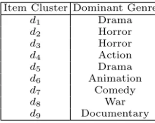
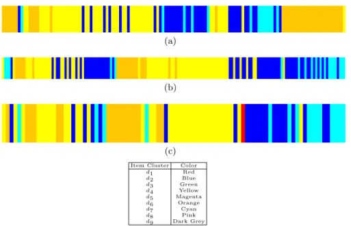
The relationships between groups of users and items captured by the BMM can be easily recognized by analyzing the distribution of the preference values for each cocluster. Given a co-cluster _{hk, li, we can analyze the} correspond-ing distribution of ratcorrespond-ing values to infer the preference/interest of the users belonging to the community k on item of the category l. Figure 3.3 shows graphically a block mixture model with 10 users clusters and 9 item clusters built on the MovieLens dataset. A hard clustering assignment has been per-formed both on users and clusters: each user u has been assigned to the cluster

(43)

c such that c = argmax

k=1,··· ,Kcuk. Symmetrically, each item i has been assigned to

the cluster d such that: d = argmax

l=1,··· ,L dil. The background color of each block

Fig. 3.3. Coclustering

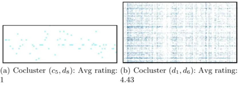
hk, li describes both the density of ratings and the average preference values given by the users (rows) belonging to the k-th group on items (columns) of the l-th category: the background intensity increases with the average rating values of the coclusters, which are given in Table 3.2. Each point within the coclusters represents a rating, and again an higher rating value corresponds to a more intense color. The analysis underlines interesting tendencies: for ex-ample, users belonging to the user community c1tend to assign higher rating

values than the average, while items belonging to item category d6 are the

most appreciated. Two interesting blocks of the whole image are further ana-lyzed in Figure 3.4(a) and in Figure 3.4(b). Here, two blocks are characterized by opposite preference behaviors: the first block contains few (low) ratings, whereas the second block exhibits a higher density of high value ratings.