POLITECNICO DI MILANO
SCHOOL OF INDUSTRIAL AND INFORMATION
ENGINEERING
MASTER OF SCIENCE IN MANAGEMENT ENGINEERING
Applying Six Sigma on private equity firms and their
assessment on the operating performance and overall
industry economic benefits
SUPERVISOR Prof. ALESSANDRO BRUN
AUTHORS
DINESH BABU KONDA RAMADOSS – 10603327
TABLE OF CONTENTS 1. Abstract
2. Implementing Six sigma in private equity firms 2.1 Introduction
2.2 What is Six Sigma? 2.3 Application of Six Sigma. 2.4 Six Sigma at IDS
3. Economic Benefits Through Six Sigma 3.1 The Hypotheses
3.2 The Test Of Hypotheses
3.2.1 Six Sigma and business improvement 3.2.2 Evaluation of Six Sigma Project by Savings
3.3 Financial based concepts to evaluate benefits of Six Sigma projects
3.4 Process for continuous evaluation of the project benefits during project life 4. Increasing returns and operating performance through Six Sigma
4.1 Methodology and Data Specification
4.1.1 Assessing Long-Run Stock Performance 4.1.2 Assessing Long-Run Operating Performance 4.1.3 The Performance of Long-Run Stock Returns
4.1.4 The Performance of Long-Run Operating Performance 4.2 Robustness Checks
4.2.1 Operating Performance Across all Six-Sigma Firms
4.2.2 Operating Performance for Company Wide Implementation 4.2.3 Operating Performance of Before and After the 2000’s 5. Summary and Conclusions
6. References
1. ABSTRACT
In recent years, companies have begun using Six Sigma Methodology to reduce errors, excessive cycle times, inefficient processes, and cost overruns related to private equity firms. This paper presents a case study to illustrate the application of Six Sigma Methodology within a finance department. The goal of the project was to streamline and standardize the
establishment and maintenance of costing and planning for all business activities within the current financial management process. The Six Sigma implementation resulted in a significant reduction in the average cycle time and cost, per unit of activity, needed to produce the required financial reports. In this study we expand the literature by looking at both financial and operational effects of undergoing through Six-Sigma trainings. We provide evidence of a four year catching up period of Six-Sigma companies listed in the Fortune 500 when adjusted for size and industry; we provide evidence of a negative mean abnormal returns following the first three years after implementation of Six-Sigma, but it becomes positive thereafter. In addition, we further analyze the effects on operating performance of undertaking Six-Sigma, also adjusted for industry and size. We only find significant statistical differences in two, out of 5 financial/operating performance aspects analyzed. Our findings, which are robust to several specifications of the tests, suggest that Six-Sigma firms, on average, are less liquid and have lower employee growth than Non-Six-Sigma firms.
2. IMPLEMENTING LEAN SIX SIGMA IN PRIVATE EQUITY FIRMS 2.1 INTRODUCTION
In 1987, Motorola developed and organized the Six Sigma process improvement
Methodology to achieve “world-class” performance, quality, and total customer satisfaction. Since that time, at least 25% of the Fortune 200, including Motorola, General Electric, Ford, Boeing, Allied Signal, Toyota, Honeywell, Kodak, Raytheon, and Bank of America, to name a few, have implemented a Six Sigma program (Antony et al. 2008, Hammer, 2002). These companies claim that Six Sigma has significantly improved their profitability (Hammer, 2002). For example, in 1998 GE claimed benefits of $1.2 billion and costs of $450 million, for a net benefit of $750 million. The company’s 1999 annual report further claimed a net benefit of more than $2 billion through the elimination of all non–value added activities in all business processes within the company (Lucas, 2002). Similarly, Allied Signal reported that Six Sigma was a major factor in the company’s $1.5 billion in estimated savings (Lucas, 2002). Six Sigma has also enabled Honeywell to reduce the development time required to redesign Web sites by 84% for its specialty materials (Maddox, 2004b). Six Sigma has been defined as a
management strategy for improving product and process quality (Hahn et al. 2000, Harry and Schroeder, 2000, Sanders and Hild, 2000). It is also a statistical term used to measure process variations, i.e., how far a given process deviates from perfection, which causes defects. Six Sigma works to systematically manage variation and eliminate defects--or to get them as close to zero as possible (Harrison, 2006). Six Sigma initiatives have typically been
implemented on shop floors of manufacturing firms to manage “process variations” (defects or errors), to improve quality and productivity (Revere and Black, 2003), and as a result, to increase the profitability of a company (Aggogeri and Gentili, 2008, Anand et al., 2007, Lucas, 2002). Functional support areas such as finance, accounting, marketing, human resources, procurement, and retail, however, have generally not kept pace with manufacturing in implementing Six Sigma programs. In part, this is due to the rigorous statistical requirements of applications that were considered too difficult to be applied within other functional areas or to predominantly service organizations (Harrison, 2006, Pyzdek, 2003, Watson, 2004). For example, in the areas of finance and accounting, Six Sigma has been used only to monitor and measure the financial impact of a program on the shop floor, in spite of the fact that,
according to a 2005 Ernst & Young study (cited in Juras et al., 2007), 14% of public companies have ineffective internal controls, which results in output errors, excessive cycle times, inefficient processes, and cost overruns. This paper presents a case study of Six Sigma as practiced in the finance department within a major division (hereafter referred as IDS) of a leading Private Equity firms. Purposes of this paper were to describe the application of the Six Sigma Methodology in streamlining the financial reporting process within the finance division of IDS, to report preliminary findings, and to examine conditions which contributed to the successful implementation. The company’s name and other attributes have been altered for reasons of confidentiality. A detailed review of Six Sigma literature was not deemed
necessary for the purpose of this case study since the literature is well known and pervasive, at least within manufacturing operations. First, this study will briefly summarize the five phases of the Six Sigma Methodology. Next, it will briefly describes the application of Six Sigma in various functional areas other than manufacturing operations. Third, the paper presents an overview of the Six Sigma initiative at IDS, to provide a context for the case
study. Finally, the actual implementation of Six Sigma Methodology in the Account Reconciliation process is discussed along with preliminary performance results.
2.2 WHAT IS SIX SIGMA?
Over the past two decades Six Sigma has evolved from a focus on metric to the Methodology level and finally to the design and development of entire Management Systems. As a Metric, when a process is operating at Six Sigma level, it will produce nonconformance (i.e., defects or errors) at a rate of not more than 3.4 defects per one million opportunities. As a
Methodology, Six Sigma leads to business process improvement by focusing on
understanding and managing customer expectations and requirements (Brewer and Eighme, 2005; Rudisill and Clary, 2004). As a Management System, Six Sigma is used to ensure that critical improvement opportunity efforts developed through the Metrics and Methodology levels are aligned with the firm’s business strategy. The focus of this paper, however, is on the application of Methodology for business process improvement within the financial reporting process. The core of the Six Sigma Methodology level is DMAIC which stands for define, measure, analyse, improve, and control. These are explained in detail in the following sections. In the Define phase, the project team must work closely with stakeholders to clearly define the problem statement, project scope, budget, schedule, and constraints. Understanding customer (internal and external) requirements is the key to achieving the project’s goal. The team has to define problems and goals of the project that are consistent with customer demands and with the firm’s business strategy. Process mapping and “voice of the customer” (VOC) tools are iterative techniques recommended as a means of
incorporating customer requirements. During the Measure phase, the team creates a value stream mapping (VSM) of the process, capturing the flow of information—where and what information is needed. Then, based on the VSM, the team starts collecting data relevant to measuring the current process performance relative to the project’s goals. The most important activities in this phase are the identification and validation of data accuracy. The most widely used tools are VSM, run charts, brainstorming, balanced scorecards,
documentation tagging, data collection check sheets, and decision metrics. During the
Analyse phase, the team needs to collect and analyse the data to understand the key process input variables that affect the project’s goal, such as whether time spent on current activities is value added or non–value added. A VMS may be used as part of the overall analysis to generate a list of potential root causes for why the process is not performing as desired. The tools that can be used are process flow chart, value stream mapping, cause-and effect diagram, Pareto analysis, histograms, control charts, and root cause analysis. During the Improve phase, the team needs to design and conduct experiments (DOE) on a small scale using a formal evaluation process to identify and evaluate optimal or desired alternatives against the established criteria. A list of all possible solutions should be developed, enabling the team to eliminate the root causes of problems. The recommended tools include
brainstorming, cost-benefit analysis, priority metrics, failure mode and effect analysis, and process flow diagrams. Finally, during the Control phase, the team should standardize and document the new process to support and sustain desired improvements. To sustain long-term improvements, how the improved process is expected to result in operational and
financial improvements (Foster, 2007) should be transparent to all employees. Tools used include statistical process control charts, flow diagrams, and pareto charts.
2.3 APPLICATIONS OF SIX SIGMA
In recent years, a number of manufacturing and service companies have realized that Six Sigma Methodology is flexible enough to be applied throughout all business functions. Examples of Six Sigma applications in different functional areas other than manufacturing operations are discussed next.
2.3.1 Sales and Marketing
In recent years, several companies have considered using Six Sigma to improve marketing processes. For example, the marketing and sales organizations at GE and Dow have been using Six Sigma for new product development and customer support to reduce costs, improve performance, and increase profitability (Maddox, 2004a). Other companies use Six Sigma in marketing and sales as a road map to capture market data and competitive
intelligence that will enable them to create products and services that meet customers’ needs (Pestorius, 2007; Rylander and Provost, 2006). Rylander and Provost (2006) suggest that companies should combine Six Sigma Methodology and online market research for better customer service, and Pestorius (2007) noted that Six Sigma could improve sales and marketing processes.
2.3.2 Accounting and Finance
The Six Sigma Methodology has made its way into the accounting function and has
contributed to reduced errors in invoice processing, reduction in cycle time, and optimized cash flow (Brewer and Bagranoff, 2004). The accounting department at a healthcare insurance provider, for instance, developed an applied Six Sigma Methodology to improve account withdrawal accuracy. Prior to Six Sigma implementation, rectifying an error in the billing process involved a number of reconciliation checkpoints and manual workflow, which resulted in 60% of customer accounts being charged less than the amount due and about 40% being overcharged. After Six Sigma implementation, the defect rate reached near zero and cycle times were reduced from two weeks to three days (Stober, 2006). The U.S. Coast Guard Finance Center used Six Sigma to create a new standardized process for accounts payable services, which improved customer satisfaction levels (Donnelly, 2007). A number of companies have applied Six Sigma to the finance process to reduce variability in cycle times, error rates, costs, “days to pay” of accounts payable, and improve employees’ productivity ratios (Brewer and Bagranoff, 2004; McInerney, 2006). Other companies have used Six Sigma to reduce the cycle time of the quarterly financial reporting process (Brewer and Eighme, 2005) and to reduce the time needed to close books, reduce variability in financial reporting, improve shareholder value, and increase the accuracy of the finance process (Gupta, 2004). Foster (2007) conducted a longitudinal study comparing the financial performance of companies who had implemented Six Sigma programs with those who did not have such a programs. He found significant effects for those firms using Six Sigma on free cash flow, earnings, and asset turnover. Six Sigma, however, did not appear to affect sales return on
assets, return on investment, or firm growth. As a result, Foster (2007) suggested if firms want to improve cash flow, earnings, or productivity in using assets, Six Sigma may of use. He also found that the companies with low cash flow and no Six Sigma programs did better than companies using Six Sigma. He suggested that for cash poor firms, Six Sigma may be a drain on resources in that these companies may not have the cash and time necessary to sustain effective Six Sigma results over time. In another industry level analysis, York and Miree (2004) studied the link between quality improvement programs and financial performance. They studied the financial performance of “quality award winning” companies against SIC control groups both before and after winning the award. They found that quality award winning firms had better financial performance both before and after winning quality awards, suggesting that winning the award was a covariate for financial success. Most studies have attempted to assess the impact of Six Sigma on financial performance have occurred at the aggregate industry level of analyses. Very few actual case studies have been reported of the impact of Six Sigma on the finance process itself. That is, how Six Sigma can change the way in which finance conducts its various work activities and the resulting impact has seldom been documented in the literature. This case study attempts to address this gap at the more micro level of within firm process analysis.
2.4 SIX SIGMA AT IDS
This case study is based on the information gathered from IDS’s implementation of a companywide Six Sigma initiative. The Six Sigma initiative at IDS was developed by
benchmarking the best practices of two other private equity firms, as well as Toyota’s Lean Thinking model, to meet the stringent standard requirements of the PE firms. The initiative at IDS received the total commitment of senior executives, a consortium of external Six Sigma experts, and a group of highly trained individuals throughout the company’s business
divisions. The Six Sigma team was comprised of a full-time master expert (Master Black Belt -- a common Six Sigma designation for the project leader) and a network of internal experts (Black Belts) working very closely with project managers. The primary goal of the team was to develop an overall Six Sigma strategy consistent with customers’ requirements and the company’s mission statement. The long-term goal of the team was to create special-level project opportunities for the division that could eventually lead to cultural change in the workplace. Forty projects were identified that encompassed the division’s business profile. Using a formal standardized metric, the team prioritized a list of project opportunities in order of their anticipated contribution to the goals of the company. In the next section, the implementation of DMAIC Methodology in one of these 40 projects i.e., the Continuing Account Reconciliation Enhancement (CARE) project is discussed in detail.
Define
Through collaborative efforts with other stakeholders in the project, the team visualized an opportunity to develop and document a standardized process for establishing and
maintaining cost and financial planning for all business divisions within its current financial system. The primary stakeholders in this project were from the finance organization, which is responsible for generating cost analyses and other financial reports for managements’
consideration. The team had the commitment of the vice president of the division, who sponsored the CARE project. The process entailed identifying undesirable or non–value added activities within the current process, implementing improvements in control systems
for achieving sustainability, and delivering measurable results that change the way people think and act. The Six Sigma team began by working with internal customers to define the objectives of the project, including the deliverable, opportunity statement, scope, schedule, budget, and constraints. The team defined the current problem as “the process cannot produce all Financial Planning and Analysis (FP&A) requirements in the most efficient and effective manner.” The primary objective of the project, therefore, was to streamline and document all cost elements in the planning process for the current financial system. To achieve the objective, the Six Sigma team recognized two primary issues. First, there was a need to clarify and simplify the current financial reporting process for internal customers by identifying all non–value added and confusing steps to reduce reporting cycle time and cost. Second, the team envisioned an improved process for both internal (called Firm contracts) and external customers (called Non-Firm) companies who outsourced their financial
reporting to IDS. The improved processes were expected to result in more timely, complete, and accurate data for planning.
Measure
At this stage, the team conducted value stream mapping analysis to measure the
performance of the current reporting process in terms of average hours required to complete the FP&A reports and the subsequent cost of preparing all the reports using activity based costing (ABC) methods. The existing cost and financial planning process was not clearly documented or consistently followed, which often resulted in rework and dual update loops, as shown in Figure 1 (Appendix). These loops inevitably create opportunities for non–value added activities such as errors, excess movement, additional IT training and maintenance costs, inconsistent data, and waiting time to creep into the process. For example, in step 1 on Figure 1, when an internal (Firm) contract was received it was entered into SAP; whereas Non-Firm business was not entered into business planning and simulation (BPS) software until it was required by the five-year plan, resulting in delays and substantial variations in the process. In step 2, when a project is not defined, it costs more and delays the process
because the finance department has to request more information (step 3). Only when a project definition was sufficiently established for a Firm for a contract, will a transaction be opened in SAP in step 4. Another problem with the existing process, step 5, was that the financial reporting for project definition was produced with data from the Business Information Warehouse (BIW), which is a combination of databases, and database
management tools that are used to support management decision making. The BIW is used in SAP and as well as other applications to support management decision making. In step 6, the project cost plans were not necessarily developed by the finance team for the program (i.e., the Cost Experts), and preparers consequently used a myriad of different financial tools (e.g., Microsoft Excel, BPS, etc.). Next, in step 7, cost element breakouts were defined using input from the various reporting tools. The Non-Firm data was added in BPS as requested by external clients, and Firm data was entered into SAP for the five-year plan FP&A
requirements. In step 8, the analysis was prepared along with reports and presentations. Finally, in step 9 the FP&A’s were revised to incorporate management change requests and both SAP and BPS data bases were updated as needed. The team found that they were spending, on average 150 hours to produce 10 internal Firm financial statements and 50 hours on 10 outside Non-Firm reports. In summary, the finance department spent a total of 200 hours to generate 20 reports (including the ongoing costs of preparing 12 monthly
reports) for an overall cost of $360,000. Using activity based-costing principles the cost of an activity is equal to: Volume x Time x Labor Cost. In this case, this would be equal to 32 reports times 200 hours times a fully burden labor costs for a total of $360,000.
Analysis
The team began this stage by creating a cause-and-effect diagram, as shown in Figure 2 (Appendix). This tool is used to identify possible root causes of why “the process cannot produce all cost and FP&A requirements in the most efficient and effective manner.” The team identified three major causes and grouped them into the following categories: 1. Lack of complete Firm cost and financial plans 2. Multiple sources of data and databases 3. Lack of complete Non-Firm cost and financial plans Next, the team used these categories as the basis for further detailed analysis to identify the contributing factors for each major cause, as shown in Figure 2. For example, one of the major causes related to the “Lack of Firm complete cost and financial plan” (activity 1) was attributable to: a) incomplete costs being entered into BPS and SAP for all businesses within the division, b) the current project cost plans were defined in various, inconsistent formats at the discretion of the finance
managers, c) the cost element plan was not required for contracts to be established in SAP. Furthermore, planning was done using multiple tools and was not copied into or maintained in a common centralized database. Additionally, planning was not consistently performed at the cost-element level because it was not previously considered necessary for FP&A
requirements. Hence, the analysis concluded that planning was not required for contracts to be established in SAP, nor was it necessary for FP&A requirements. The team used VSM analysis to recommend the following actions for overall process performance improvement: 1. Identify all business divisions that require a baseline in the current financial database. 2. Establish baseline data by resource, cost element, and time phasing for each project. 3. Identify and eliminate all non–value added activities to improve the response time at all levels of management for a variety of cost analysis and FP&A requirements, including five-year plans, bookings forecasts, sales forecasts, and annual operating plans.
Improve
In this stage, the team provided two solutions for implementation by the finance department. First, implement all the actions identified through VSM analysis. Second, redesign the process by following the flow chart shown in Figure 3 (Appendix) which essentially simplified the process by eliminating non-value added steps in the current process.
In addition, the Six Sigma team recommended that all business divisions be required to implement the following actions to enhance financial reporting capabilities:
1. Develop initial cost-element plans by project for both internal and external contracts.
2. Regularly copy cost plans to various FP&A versions for five-year planning, sales forecasting, and bookings forecasting.
3. Update and maintain cost-element plans as new businesses are identified and funding is received.
4. Update and maintain financial plans.
5. Copy updated financial plans to various FP&A versions accordingly.
After implementing the recommended process changes and actions, the following results were achieved: • Cost-element and financial planning activities for all business divisions were standardized, consistently created and maintained in a centralized database;
• Processes were streamlined, documented, and consistently followed throughout the reporting process;
• Significant reduction in cycle time was achieved for producing the FP&A reports;
specifically, the revised process resulted in 100 hours reduction in cycle time, resulting in cost savings of $130,000 per year or roughly a 64 percent reduction.
A cost savings of $130,000 may not appear to be much considering the cost of Six Sigma implementation, but recall this is only one of forty projects within the finance function. In reality, the reported cost savings of $130,000 a year is actually cost avoidance. That is, in order to increase profitability one must lower cost by, for example, reducing headcount through attrition or by absorbing future increases in the volume of work but with the same labor costs.
Control
The goal of the project was to pull cost elements and financial plans from their various sources, organize them, and combine the information into one comprehensive report for analysis and monthly program presentations. To sustain results, the team standardized, documented, and distributed the new process for the finance department to follow. Additionally, ongoing performance was monitored and became part of the formal performance evaluation process.
3. ECONOMIC BENEFITS THROUGH SIX SIGMA
Today, companies and industries are under increasing pressure to reduce the costs while the business performance has to improve. The objective related to the business improvement is for the top management obvious: maximization of shareholder value through increased profits.
The activities to assure quality in a company can be grouped in three processes: quality planning, quality control and quality improvement (Juran & De Feo, 2010). Quality improvement activities does not enhance the quality level only but leads to the cost’s optimization, improvement of market share or a pricing effect. These outcomes have positive effect on the company profit. From another – production – perspective long-term performance of a manufacturing company depends on quality and efficiency of the production processes therefore the improvement in this area has the positive effect on the profit as well. In addition, a quality improvement program leads to the creation of the product that customer values, so the customer satisfaction increases as another important long- term success indicator for a company.
3.1 THE HYPOTHESES
Quality improvement activities are executed in projects and this systematic project base distinguishes quality improvement from quality control, which is based on the reactive approach. Several quality improvement strategies, which are statisticaly based have been developed, in order to guide quality professionals to perform improvement projects. The most frequently used are the Six Sigma methodology, the Shainin System and Taguchi’s methods.
The selection of the quality improvement projects in the rapidly developing industries such as automotive or electronics suggests evaluation of effort and resources allocated to the project in order to deliver maximum benefits to the company. Project selection process have become crucial as the effectiveness of
the quality improvement programs is one of the key factors for the fulfilment of the business objectives and development of the employees.
The way the Six Sigma methodology is used has changed in last few years. The influence of the economic crisis led to the situation the improvement programs are evaluated more strongly by economic criteria. In the past the Six Sigma programs were not defined based on the economics aspects primarily but rather on a confidence or a trust the quality improvement can bring a positive effect. Six Sigma was taken as a quality initiative that does target the cost reduction secondarily. It means the quality improvement could save money by eliminating of the defective products, rework or returned products but this was taken as a by- product of the project.
In this paper we will seek for the estimation of benefits coming out of an improvement project especially focusing on Six Sigma projects.
3.2 TEST OF HYPOTHESES Six Sigma methodology
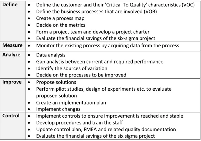
Six Sigma is a robust continuous improvement strategy that rely on statistical methods. But Six Sigma is more than a set of tools. Six Sigma is the strategic and systematic application of the tools on a project in order to reach significant and long-term improvement. In general, Six Sigma methodology solves the process or business problem by reduction of the variation (Nave, 2002). Six Sigma methodology provides a structured data-driven approach based on statistical methods that companies use to measure their performance both before and after an improvement project. No changes are made until the current process is completely understood, documented and measured. The revised process is measured and verified after the improvement action is finished. Apart from that we have to consider Six Sigma as the approach strongly focused on the customer needs. Basically, the DMAIC process translates customer requirements into operational terms and defines the processes critical to quality which must be completed to meet customer needs (Juran & De Feo, 2010). Six Sigma methodology consists of five steps known as DMAIC process (Table 1).
Table 1 – DMAIC structure of Six Sigma strategy
Define • Define the customer and their 'Critical To Quality' characteristics (VOC) • Define the business processes that are involved (VOB)
• Create a process map • Decide on the metrics
• Form a project team and develop a project charter • Evaluate the financial savings of the six-sigma project
Measure • Monitor the existing process by acquiring data from the process Analyze • Data analysis
• Gap analysis between current and required performance • Identify the sources of variation
• Decide on the processes to be improved Improve • Propose solutions
• Perform pilot studies, design of experiments etc. to evaluate proposed solution
• Create an implementation plan • Implement changes
Control • Implement controls to ensure improvement is reached and stable • Develop procedures and train the staff
• Update control plan, FMEA and related quality documentation • Evaluate the financial savings of the six sigma project
3.2.1 Six Sigma and business improvement
To select a beneficial improvement project a company has to to work with two main inputs: Voice of Customer (VOC) and Voice of Business (VOB). VOC is the most powerful input. Why VOC is so strong? The reason is obvious: the customer is the reason to run the business. Significant portion of the Six Sigma projects is initiated based on customer request or, in the worst case, on customer complaint. Voice of Business (VOB) is an inner voice of the company. Perhaps it is not as strong voice as VOC but many improvement actions and activities have arisen from the identification of the internal needs and gaps within the processes.
These two voices are linked together through process output that has to comply with requirements specified internally by business needs and externally by customer requirements. Properly selected Six Sigma project will be in line with customer expectation and business priorities if the VOC and VOB is reflected. This would guarantee the validity and the priority of the project which can be recognized by management.
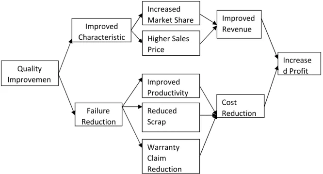
A quality improvement activity brings two main effects: improvement of the product characteristics and failure reduction. A real quality improvement should end up by the economical benefit represented increased profit at the end (see Figure 1).
Maximum price
Price range
The improvement of the production quality and product quality leads to the high production efficiency, prevention of the scrap and decreasing of the process variance. The costs of poor quality are minimized and thereby the production costs are lower so unit costs are decreased as well. Higher internal quality contributes to low level of external failures. It causes the external effect as customer satisfaction increases due to low defect rate of the product in the market.
The better quality can have a positive effect on the pricing as customer will start to distinguish between low- and high-quality product as shown on Figure 2 (Freiesleben, 2004).
Figure 1 – Economics of a quality improvement project
A B Quality
Lower level of quality Higher level of quality
Warranty Claim Reduction Reduced Scrap Improved Productivity Failure Reduction Quality Improvemen t Higher Sales Price Improved Characteristic Increased
Market Share Improved Revenue Cost Reduction Increase d Profit Un it pri ce
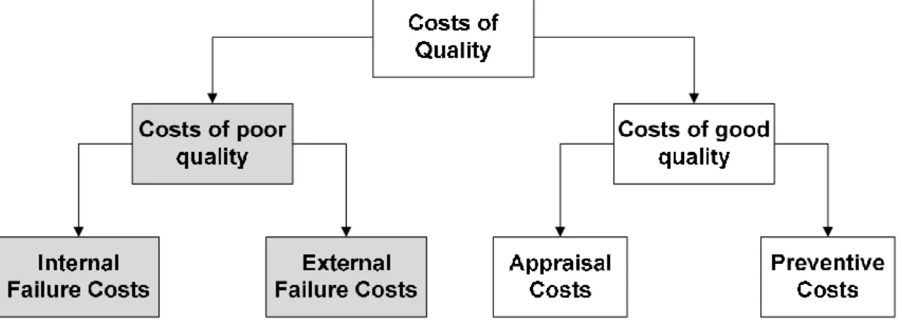
Quality improvement is linked to quality costs. The structure of the quality costs can be explained by traditional quality costs model, (PAF model, Prevention- Appraisal-Failure model) which defines these costs consisting of four costs categories: internal failure costs, external failure costs, appraisal costs and prevention costs. (Nenadal, 2004). Total quality costs are the sum of the costs of poor quality and the costs of achieving good quality then (see Figure 3).
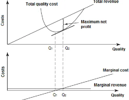
The analysis of the costs of poor quality itself does not create a good base for the financial evaluation of the quality improvement project. The reduction of the quality costs will minimize the production costs, but this analysis will not demonstrate the contribution to the profit increase (Miller & Morris, 2000). The missing link between benefits and costs of poor quality is revenue (Figure 4). As shown in Figure 1 revenue can be increased if market share is increased and/or the price is heightening. In Figure 4 revenue is shown as increasing function of quality. Net profit of the company is the difference between total revenue and total quality costs. Point Q1 represents the quality level with total costs of quality being minimized. Profit maximization is reached in the point Q2. Further improvement of the quality between Q1 and Q2 causes the slight increase of the total quality costs however the slope of the total revenue line is steeper therefore the additional profit is created The lower graph illustrates the same situation displaying marginal values of the revenue and costs in relation to quality. Marginal lines represents the slope of the absolute characteristics: marginal costs shows the slope of the total costs line and marginal revenue is equal to the slope of the total revenue line. Revenue exceeds marginal costs in point Q1 so at minimum costs of quality.
Figure 3 – Costs of quality structure (PAF model)
3.2.2 Evaluation of Six Sigma projects by savings
The assessment of the project benefits using revenue or net profit is not an easy part especially for green belts. The financial impact of the individual Six Sigma project is evaluated through savings. The project charter of each Six
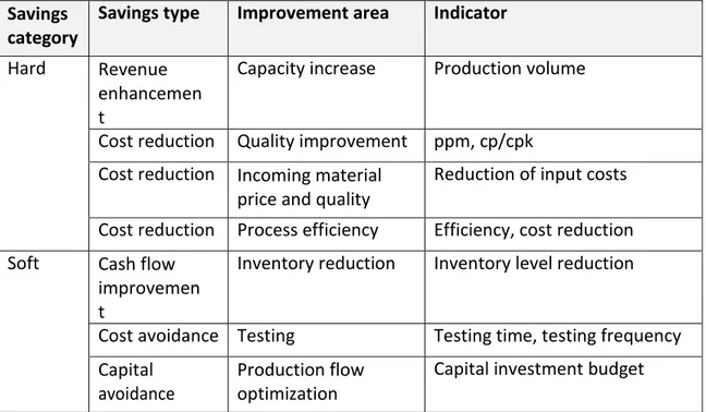
Sigma project should show the overview of the expected savings in the Define phase already. Two groups of Six Sigma savings are defined: hard and soft. Hard savings influence the year-to-year financial results, reduce spending and budget variances. The hard savings are categorized as cost reduction and revenue enhancement. Soft savings improve the cash flow, impact future capital budgeting and they may influence the capital spending. There are three categories of the soft savings: cash flow improvement, cost and capital avoidance (Snee & Rodebaugh, 2002).
Figure 4 – Quality costs versus revenue
Explanation: Q1 – the quality level with total costs of quality being minimized; Q2 –
profit maximization
Although savings are well defined from economical point to assess the project savings is the most difficult point for green belts and black belts and it could become blocking point to start a project. Why is this point so painful? Most of the green belts and black belts are employees with technical background but with low knowledge regarding business economy. If we look at the agenda of a Six Sigma green belt or black belt course we will find sporadic information about business economics related to the Six Sigma methodology. Not sufficient economical knowledge leads to the fact the green belts and black belts are trying to link their Six Sigma project to a most obvious saving. The simplification does not allow proper project rating as one project influences several categories of savings usually. The situation is more complicated with soft savings which are difficult to recognize and quantify.
Table 2 – Savings categories
Savings category
Savings type Improvement area Indicator Hard Revenue
enhancemen t
Capacity increase Production volume
Cost reduction Quality improvement ppm, cp/cpk Cost reduction Incoming material
price and quality
Reduction of input costs Cost reduction Process efficiency Efficiency, cost reduction Soft Cash flow
improvemen t
Inventory reduction Inventory level reduction
Cost avoidance Testing Testing time, testing frequency Capital
avoidance
Production flow optimization
Capital investment budget
3.3 Financial based concepts to evaluate benefits of Six Sigma projects
The most popular concept (and to be honest the one which is usually explained on the green belt/black belt course) is known as hidden factory. This concept is based on the elimination of so called hidden factory costs. Example: we have to produce x good products and our actual defect rate is q. To fulfill customer needs for delivered volume (v) we have to produce volume
v = x / 1 – q,
If we consider c as variable cost per unit then related variable costs C = c(v-x)
are indirect costs of poor quality caused by overproduction (Bisgaard & Freiesleben, 2000). The calculation of the cost savings related to Six Sigma project could be simplified using this concept as hidden factory costs are equal to the savings. This simplified way of calculation ignores the investment to the improvement of the process. The improvement action has long-term effect while spending related to improvement could be taken as a one-time investment. From accounting point of costs related to investment will be written off for certain time. This allows us to evaluate the benefit of Six Sigma program by return of investment (ROI) calculation.
Unadjusted return of investment can be expressed by formula (Bisgaard & Freiesleben, 2000):
ROI = 100.(operating advantage - amortization) / Investment
(3) This calculation does not include the interest rate in to judgement.
The expectation related to the usage of the ROI as the criteria for the evaluation of the benefit of Six Sigma program is one time investment. This condition comes true for green belt projects which take approximately three to six months to complete. The situation differentiates from ongoing long-term improvement activities. Leading companies implemented different approach to improve the quality of their product based on the continuous, systematic innovation strategy. Such strategy can contain process innovation, product innovation as well as radical and incremental innovation (Bisgaard & De Mast, 2006) . The innovation strategy is executed by the structured improvement programs where the Six Sigma is used as an engine to run the improvement process. An advanced innovation programme starts in the design phase already where the Design for Six Sigma (DFSS) approach can be used to set up the appropriate quality level and economical effectiveness of the product and process prior production phase. These improvement activities have to be evaluated from economical point as long-term projects that have different cash flow developing over several years. The net present value (NPV) could be suitable characteristic to evaluate such long-term activity. The expected future incomes and outcomes are converted to current value using an estimated rate taking in account the “time value of money”. The NPV can be expressed by the formula:
NPV = ∑ investment value / (1 + rate)^2.
Investment value is the sum of the costs and revenues related to investment realization, n represents individual years of the investment utilization, t means total investment utilization and rate is related to the alternative valorization which reflects amount of interests (Kral, 2010).. Even the formula looks simple I would strongly recommend to ask financial department for the support in case of the evaluation of NPV.
There are further methods the financial impact evaluation of six sigma projects which are even more based on the accounting approach i.e. EVA method (Mader, 2009).
3.4 Process for continuous evaluation of the project benefits during project life time
The financial benefits are the key aspects of the Six Sigma projects which have to be taken in consideration before a project is launched. Unfortunately there is no simple way how to calculate the financial benefit coming out of the project. The idea the cost savings being assessed by green belts or black belts themselves does not bring a value usually. The only effective solution is to involve finance department in the evaluation of the Six Sigma project from an early phase. This is nothing revolutionary new: a Six Sigma project has to be simply traced any
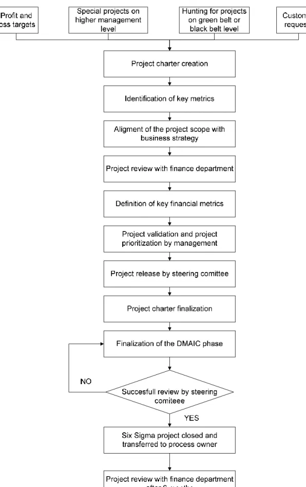
valuated as any other project in the company. The financial metrics are just implemented as the key performance indicators of the project. The most effective way to evaluate benefits of Six Sigma projects is to create continuous project evaluation process to maintain the tracking of project development closely. At the beginning of the project the key metrics are defined in the project charter which has been created as soon as the project idea is generated. Well-defined project charter outlines the scope of a project, financial targets, anticipated benefits and. In the initial phase it is important to generate the metrics by green belt and black belt. The financial metrics are reviewed with finance department taking in account product life cycle phase, complexity and expected duration of the project, expected investments, hard and soft savings. The project pre-agreed with finance department is submitted to Six Sigma steering committee to decide about release of project for execution. The status of the project is reviewed after each milestone of the project (Define, Measure, Analyze, Improve, Control milestone at least) including the financial indicators. The project status at the point of milestone is the key decision point (but not only one) to differentiate the projects with high benefit potential from projects with low expectation. The final evaluation of the Six Sigma project benefits is done six months after the project closure. The complete flow describing the process of continuous evaluation of the Six Sigma benefits is shown by Figure 5.
26 4. Increasing returns and operating performance through Six Sigma
Managers are increasingly held accountable for delivering maximum shareholder value while also providing an improved relationship with stakeholders, and particularly customers. Since the
1980’s,industrial organizations have adopted quality control practices, such as Six Sigma, to maintain and enhance competitiveness. According to Derming (1990) most failures in organizations are caused by systemic flaws rather than individual errors, which prevent companies from achieving levels of quality, or productivity, that companies might otherwise be capable of achieving. Bacidore et al. (2005) discuss that a quality control programs have:
Six-Sigma is currently one of the most popular quality management programs to date. Researchers describe Six Sigma as a data-driven management strategy focus on problem solving based on statistical analysis (Blakeslee, 1999; Hahn et al., 1999; Harry and Schroeder, 2000; Braunscheidel et al., 2011). This quality control process can be viewed as an attempt to communicate organizational attributes to parties, customers and investors, who cannot observe them directly. Although the literature has focused on the effects of the quality improvements on the business process itself, little attention has been given to the financial outcome of incorporating these practices; financially speaking, quality control programs must be translated into larger profits and increased shareholder wealth which is, after all, the fiduciary duty of managers and the board of directors.
The net operating effects of these types of investments have not been rigorously examined. Most scholarly work to date involves perceptual data from surveys, or financial studies of a few select companies (Goh et al., 2003; Zu et al., 2008; Gutierrez et al., 2009; Braunscheidel et al., 2011). In this paper, we expand the literature on the financial effects of operations management by employing a larger dataset, both in number of firms analyzed and the time frame of the study, of companies that have implemented Six-Sigma. We assess the financial consequences of undertaking Six-Sigma principles by comparing the long-run stock performance and operating performance of Fortune 500 companies with and without Six-Sigma principles.
The Six-Sigma approach, formulated by Motorola in the 1980s, can be synthesized in improving the capability of business processes by using statistical methods to identify, decrease, or fully eliminate process variation to no more than 3.4 defects per million (Motorola 2009). It is expected that by reducing defects in production, thereby improving product quality, employee morale and ultimately profits will soar. Simply put, adopting Six-Sigma would improve the organizational performance through higher employee productivity without negatively affecting the company’s performance (Shafer and Moeller, 2012). In this regard, companies are willing to invest large amounts of capital in such quality management systems; training costs can be as high as $50,000 per worker (Antony, 2006; Fahmy, 2006) increasing training expenses to upwards of $1.6 billion as it was the case of General Electric (Feng, 2008).
Six-Sigma appeared as a response to the fact that organizations with poor processes management are less effective than those that do (Kaplan and Norton 2001). Without specific quality control processes,
organizations rely on learning-by-doing which takes longer times of improvement (Aldrich and Ruef, 2006). The objective of Six-Sigma is thus to eliminate inefficient steps through check sheets, Pareto
27 analysis, cause and effect diagrams, root cause analysis, and value added analysis, among others (Conger, 2015)1. And these administrative innovations affect the ways that organizational members conduct their routine work (Sinha and Van de Ven, 2005).1997, Citibank hired Motorola University Consulting and Training Services to teach Six Sigma to 650 senior managers. Moreover, between November 1997 and the end of 1998, another 7,500 senior-manager-led teams were trained. And by early 1999, a total of 92,000 employees worldwide had been trained. Furthermore, Six-Sigma has even been adopted by many firms that had already possessed quite mature quality management processes like 3M, Ford, Honeywell, and American Express (Schroeder et al., 2008). Currently, most Fortune 500 companies have invested in Six-Sigma training (Nakhai and Neves, 2009).
Still, there is a cast of doubt surrounding the efficacy of Six-Sigma. For instance, research has shown that corporate improvements could be due to social aspects (Powell, 1995), a supportive learning culture (Detert et al., 2000; Schroeder et al., 2008; Naor et al., 2008), implementation of a shared vision (Gutierrez, et al., 2009), and/or cooperative values (Kull and Narasimhan, 2010), rather than a direct consequence of the Six-Sigma training. Furthermore, many researchers have questioned the
effectiveness of adopting Six-Sigma (see: Abernathy, 1978; Tushman and O’Reilly, 1996; Clifford, 2001; Benner and Tushman, 2002; Rowlands, 2003; Goh et al., 2003; Naveh and Erez, 2004; Zu et al., 2008). Finally, managers from General Electric and 3M suggested that Six Sigma practices may have constrain innovation needed to drive growth (Rogers, 2003; Brady, 2005; Hindo, 2007).
But the literature shows supporting evidence of a positive effect of adopting Six-Sigma. The benefits range from effective cost savings (Pande et al., 2000; Harry and Schroeder, 2000, Braunscheidel et al., 2011) and innovation (Braunscheidel et al., 2011), to increased return on investments (Dorgan and Dowdy, 2004; Swink and Jacobs, 2012), to enhanced overall performance across different business aspects (Jacobs, Swink and Linderman, 2015). In fact, post-adoption of Six-Sigma, firms show that overall quality is improved in both production (Ittner et al., 2001; Choo et al., 2007; Molina et al., 2007; Swink and Jacobs, 2012;), as well as job quality (Linderman et al., 2003 and 2006; Levine and Toffel, 2010)
Although the literature shows proficiency looking at the effects of quality controls, to our knowledge, no prior research has extensively looked at all areas of the business from operations to profitability to stock prices. It remains uncertain whether Six-Sigma enhances profitability given that it is exclusively a
customer-driven system (Breyfogle, 2003) which emphasizes on customer-oriented metrics (Linderman et al., 2003; Sinha and Van de Ven, 2005; Schroeder et al., 2008). Moreover, it is necessary to look at the long term performance of companies which have adopted Six-Sigma, given the evolving nature of processes over time (Robertson et al., 1996; Rogers, 2003; Strang and Kim, 2004). Companies must first learn to understand the specific business processes before they can remove excess (vom Brocke et al. 2010).
In this regard, we provide an analysis of the effects of adopting Six-Sigma practices within the 2006 Fortune 500 companies. This provides a sample of 108 companies that were identified as having implemented Six-Sigma. We then estimate five-year performance metrics for the 108 Six-Sigma companies and 398 non-Six-Sigma companies. Our study is split into two parts: (1) long-run stock performance and (2) long-run effects on operating performance.
28 Our findings suggest that Six-Sigma companies outperform the market, as evidenced by positive mean abnormal returns and mean buy-and-hold returns for every year during the window [−3, +5] years, where 𝑡0 is the implementation year. Furthermore, we find supporting evidence suggesting that Six- Sigma firms go through a catching up period of four years before outperforming companies matched by size and industry. But since this positive difference only appears four years after the adoption of Six- Sigma, we caution the reader because a direct causality of this over-performance of Six-Sigma firms is not proven.
In comparison, our findings are somehow aligned with those of Goh et al. (2003) and Zu et al. (2008). Goh et al. investigate, based on a sample of 20 firms, stock price reactions on the day when Six-Sigma
activities are made known publicly, as well as the long-run stock performance of those companies. They report no significant increase in returns surrounding the announcement date or an abnormal long-term performance increase. Moreover, Zu et al. find that the long run stock performance of Six-Sigma firms is not better than the S&P 500. Further examples of the reactions to Six-Sigma announcements include Ramasesh (1998) and Przasnyski and Tai (1999).
In addition to stock performance, we look at operational performance. We investigated the effects of undertaking the Six-Sigma principles on fourteen ratios dealing with liquidity, activity, management, earnings, and labor. We can only find statistical significance in ratio performance for 2 out of 5 areas: liquidity and labor performance. The evidence suggests that Non-Sigma firms are more liquid than Six-Sigma firms before and after the training, which is of statistical significance at the traditional levels. Also, the only significant difference is given by growth in staff, but only after the implementation of Six— Sigma; we find a decrease of 8% in staff over the 5 years following the implementation of Six-Sigma. Altogether, there is no evidence of superior operational performance of Six-Sigma companies despite the reduction of personnel. Our findings are robust to reducing the dataset to account only for company- wide adoptions, early adoptions,
It is worthwhile noting that the literature shows other non-quantitative desired effects of undertaking Six-Sigma. For example, the literature shows that Six-Sigma practices requires structured improvement methods which lead to better organizational learning and knowledge transfer (Ittner et al., 2001; Choo et al., 2007; Molina et al., 2007; Swink and Jacobs, 2012), as well as overall improved job quality (Levine and Toffel, 2010), and that the interaction of the structured method and rigorous goal setting of Six Sigma explains its impact on the performance of specific projects (Linderman et al. 2003 and 2006).
Additionally, De Mast and Lokkerbol, 2012, argue that Six-Sigma itself is a generic process, and that research should focus on the implementation of DMAIC2 processes. Furthermore, newer research has focused on the adoption of Lean Principles to Six-Sigma, ergo Lean Six Sigma (see: Hilton and Sohal., 2012; Assarlind, et al., 2013; Antony, 2015). But such questions, including the analysis qualitative benefits, are beyond the scope of this paper and is left for future research.
The remaining of this paper remains as follows: section 2 describes the data description of both the Six-Sigma and the matching non-Six-Six-Sigma companies, as well as the methodology used to assess long- run
29 stock performance and the description of an event study methodology used to assess operational performance; section 3 provides a summary of our findings; section 4 then develops several robustness checks; and finally section 4 provides concluding remarks.
4.1 Methodology and Data Specification Data
We hand collected public financial data from the companies listed in the Fortune-500 2006 report, and identify the list of companies which have adopted Six-Sigma practices. This process results in a dataset containing 108 companies. In addition, the 108 Six-Sigma companies are adjusted for relative
performance by adjusting for size and industry within the 2006 Fortune 500 listing. That is, each Six-Sigma company is paired with a Non-Six-Sigma company. This matching is done on a one-to-one bases based on the SIC 3-digit code for industries and within a 30% size adjustment.
We, therefore, gather yearly SEC filings for three years before and five years after the reported Six- Sigma implementation; this results in a dataset with yearly financial data from 1984 through 2013. But because the data spam is focused on three years before and five years after the implementation of Six- Sigma, all data is centered on the implementation date, 𝑡0 = 0; thus creating and event-window [−3, +5] years. Finally, because we use yearly data, all event windows are centered on December of the implementation year (𝑡0 = 𝐷𝑒𝑐𝑒𝑚𝑏𝑒𝑟 = 0).
Looking at the data, the earliest implementation reported was in 1987 (Motorola) and the latest was in 2007 (Walmart)3. Most companies implemented them in the 1990s and 2000s, where the median implementation date is 2001. It is thus interesting to analyze the difference between implementation periods to test the advantages of early adoption. We therefore split the sample into pre- and post-2001 implementation to account for possible advantages of early movers.
Moreover, we recognize 4 levels at which companies can implement Six-Sigma: (1) the corporate level which is an enterprise-wide initiative with corporate commitment and support; (2) the business unit level which is deployment and support by a corporate executive or business unit executive; (3) the pilot level which describes trial initiatives in a selected business unit; and (4) the belt level which is limited to selected projects organized around personnel who have green belt or black belt certification. Of the 108
companies, eighty-five had implemented Six Sigma at the corporate level, fourteen at the business unit level, four at the pilot level, and five at the belt level. Finally, data regarding stock prices is included to assess financial performance. We download monthly pricing data for all 216 companies from CRSP. Once again, this is done based on a [−3, +5] window centered around 𝑡0. Furthermore, we include the returns on the S&P500 from 1984 to 2013, as it is always required to have a benchmark for average market performance.
Based on this data, we tests two hypothesis: (1) we look at the long-term stock performance of Six- Sigma companies using average cumulative abnormal returns and buy-and-hold returns, and (2) we look at the overall effect on operating performance of Six-Sigma firms, by doing an event study based on their financial ratios pre- and post- adoption of Six-Sigma. Our expectation is that Six-Sigma adopters will
30 𝑇
𝑇
perform better not only operationally, but also financially. We report our results based on the size- and industry-adjusted performance and unadjusted performance. The following sub-sections describe the methodology for testing both hypothesis.
4.1.1 Assessing Long-Run Stock Performance
We start by defining market-adjusted monthly abnormal returns as the difference between a firm’s return and the benchmark; formally:
𝐴𝑅𝑖,𝑇 = 𝑅𝑖,𝑇 − 𝑅𝑆&𝑃500
where 𝐴𝑅𝑖,𝑇 is the abnormal return of stock 𝑖 in month 𝑡, 𝑅𝑖,𝑇 is the return of stock 𝑖 at month 𝑡, and 𝑅𝑆&𝑃500 is the market return, based on the S&P500 index, during month 𝑇. Since the objective is to estimate long-term performance, we estimate both: expected equally weighted abnormal returns and buy and hold abnormal returns.
While the expected return is just a measurement of the long term average performance over a particular investment period, the buy and hold return shows the actual amount of money generated. Thus,
following an event study centered on the company’s Six-Sigma adoption date, we define event windows not only to differentiate between pre- and post-adoption performance, but also between different stages of the adoption process. It is worthwhile noting, however, that 𝑡 = 0 varies depending on the year on which the company decided to implement the Six-Sigma training; but the event window itself remains thus constant.
We estimate a total of 8 different event windows. The first three windows define the pre adoption period: [−36,0], [−24,0], and [−12,0]; and the remaining five define the post-adoption period: [0,12], [0,24], [0,36], [0,48], and [0,60]. Formally then, expected cumulative abnormal returns are defined as: 𝑇 𝐴𝑅𝐸 = 1 ∑ 𝐴𝑅 , 𝑖 𝑁 𝑡 𝑖,𝑇
31 and buy-and-hold returns are defined as:
𝑇 𝑇
𝐴𝑅𝐵𝐻 = ∏(1 + 𝑅𝑖,𝑇) − ∏(1 + 𝑅𝑆&𝑃500) ;
𝑖 𝑇
𝑡 𝑡
where [𝑡, 𝑇] represents the particular event window. 4.1.2 Assessing Long-Run Operating Performance
Next, we examine the relative operating performance of firms that adopted Six-Sigma to the remaining Fortune 500 companies. For robustness, we match the 108 Six-Sigma firms in the dataset to industry- and size-matched companies. Five different measures of operating performance are, thus, analyzed: liquidity analysis, activity analysis, management efficiency, earnings ability, and labor. This results in fourteen total ratios being analyzed. Table 1 summarizes the estimation of all rations, while details sustain the rationale of using these ratios are explicated in Appendix A.
[TABLE 1 ABOUT HERE]
All ratios are estimated based on the same full event-window described above: [𝑡 = −3, 𝑡 = +5], on yearly bases. We also use two extra event windows to differentiate between pre- and post-adoption periods: [𝑡 = −3, 𝑡 = 1] and [𝑡 = 1, 𝑡 = +5]. The actual effects on operating performance are therefore examined by comparing the Six Sigma firms’ ratios from both pre- and post-implementation windows.
Researchers maintain that a firm must possess certain resources and make certain commitments in order to make Six Sigma successful. Hence, Six Sigma methods and tools may be more or less effective in
certain technological and operational contexts. (Antony et al., 2008; Schroeder et al., 2008; Jacobs, et al. 2015). Therefore, to account for the possibility that the ratios may, indeed, be biased in favor of certain companies4, industry- and size-adjusted median ratios (performance) are reported. The Industry- and size-adjusted performance is calculated as the difference between the ratios for Six-Sigma firms and ratios for the matching firms described above.
Moreover, each year, companies and their adjusting firms are ranked based on the performance of each ratio. This results on 108 matching pairs per year within the testing period [−3, +5]. Following Otchere (2005), who uses the Wilcoxon (1945) signed-rank test, we estimate a w-test-statistic5 for differences in median performance within the pairs. This is based on a z-test statistic because 𝑛 is sufficiently large; that is, the critical 𝑧 − 𝑣𝑎𝑙𝑢𝑒 is given by:
32 𝑤 − 𝑛(𝑛 − 1)
𝑧 = 4
√𝑛(𝑛 − 1)(2𝑛 − 1) 24
Finally, we test for a change in the mean/median performance between the pre-Six Sigma period (window [−3, +1]) and the Six Sigma period (window [+1, +5]); we separate between pre- and post-adoption periods at year 1 to allow changes to take effect before analyzing the results. This is done by performing a t-test of differences in means.
Results
4.1.3 The Performance of Long-Run Stock Returns
The long-run stock performance of sample firms is examined by analyzing three different mean returns,
viz., market-adjusted returns, buy-and-hold returns, and unadjusted returns of firms that have
implemented Six Sigma versus industry- and size-matched firms. It is expected that the Six Sigma process compels management to pursue process improvement and cost-cutting projects that will enable firms to generate higher returns for investors.
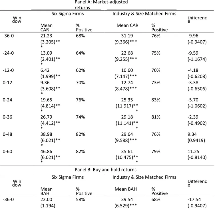
Table 2 summarizes the stock returns for the 108 companies that implemented Six-Sigma along with the industry- and size-matched firms. Panel A shows the mean abnormal returns and Panel B shows the buy-and-hold abnormal returns. To analyze the timely effect of adopting Six-Sigma, all returns are reported for all the suggested event windows: [−36,0], [−24,0], [−12,0], [0,12], [0,24], [0,36], [0,48], and [0,60]. In addition, for comparison purposes, Table 2 Panel C reports unadjusted returns. Finally, all findings are tested for a null hypothesis of zero abnormal returns based on a t-test.
[TABLE 2 ABOUT HERE]
Rapid inspection shows that Six Sigma firms always outperform the market, regardless of the event period; though it is not statistically significant for the [−36,0], and [−24,0] windows. Still, buy-and-hold returns are significantly higher than the S&P 500 after implementing Six Sigma: the results show a 7.48% mean buy and hold return after the first year, which increases to 48.34% over the five years after the implementation. All results are statistically significant at the one percent level, except for the [0,12] window which is significant at the 5% level.
But more importantly, Six-Sigma returns are compared to industry- and size-matching firms within the Fortune 500. This is estimated as the difference 𝑅𝑁𝑜𝑛𝑆𝑖𝑥𝑆𝑖𝑔𝑚𝑎 − 𝑅𝑆𝑖𝑥𝑆𝑖𝑔𝑚𝑎. Based on market adjusted returns, the results suggest that Six-Sigma firms need at least three years to catch up, and perform better, than the matching firms, as evidenced by a negative difference during windows [0,12], [0,24], [0,36] and subsequent positive difference thereafter. But it is worthwhile noting that, on average,
33 Non-Six-Sigma firms outperformed Six-Sigma firms even before the latter firms implemented the Six- Sigma process.
For controlling purposes, unadjusted mean cumulative returns are also analyzed. The evidence suggest that Non-Six-Sigma companies perform better. This is true regardless of the period of analysis. The cumulative return over the three years before the implementation date is reported to be 50.81% for the Six-Sigma firms, while the matching firms provided a 57.35% over the same period. Moreover, over the five years after the implementation, the cumulative returns of Six-Sigma firms is 66.23%, which is 4.30% lower than the matching firms.
Overall, this does not provide strong supporting evidence of a long-term improved financial performance post Six-Sigma implementation. Although the evidence suggest that stock returns do increase four years post the implementation process, we caution the reader given the plausible existence of other external factors directly causing this improvement. We further this discussion in the following section by looking at financial performance across different areas of the business.
4.1.4 The Performance of Long-Run Operating Performance
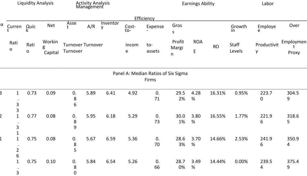
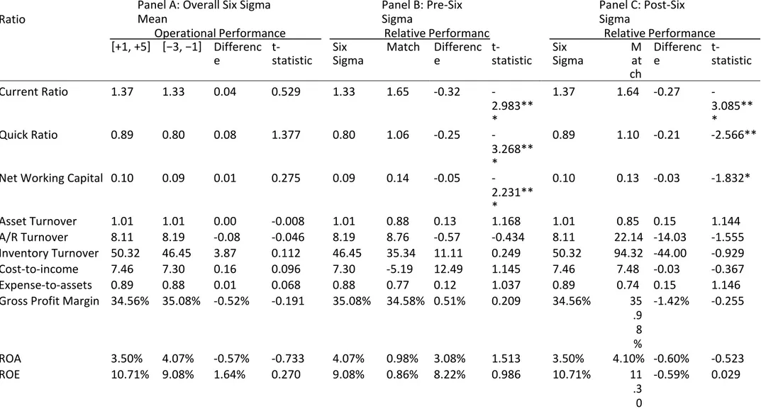
In this section, we analyze the proposed five different measures of operating performance. We estimate 14 financial ratios to signal the effects on liquidity analysis, activity analysis, management efficiency, earnings ability, and labor. Table 3 summarizes the results. Panel A describes the yearly median ratios for the 108 Six-Sigma companies, while Panel B summarizes the results for the matching firms. For
comparison purposes, the Wilcoxon test is included in Panel C.
The results show that Six Sigma firms have lower liquidity than matching firms across all years.
Considering the implementation year, 𝑡0, liquidity for Six-Sigma firms is lower than the liquidity of the matching firms, but not statistically significant except for the quick ratio; this is expected if the investment is made with liquid assets. But there is not sufficient evidence that liquidity improves even after 5 years after the implementation of Six-Sigma; in year five, the current ratio is estimated to be 1.36, the quick ratio 0.83, and the net working capital is 0.08 for the Six sigma firms in comparison to 1.52, 0.91, and 0.12 respectively6.
On the other hand, Six Sigma firms are at parity with matching firms in terms of activity analysis and management efficiency, given that the difference in ranked paired ratios is not statistically significant per the Wilcoxon test. The only events when Six-Sigma firms outperform their controlling firms, is in median inventory turnover during year 3 and year 4 after implementation; median inventory turnover ratio improves to 8.03 compared to 6.32 during year 3, and 7.86 compared to 5.98 (statistically significant at the 10% level) during year 4.
Regarding earnings, results show that Six Sigma firms have significantly higher return on equity (ROE) before implementation compared to matching firms. Three years prior to implementation, the median ROE is 16.31% for Six Sigma firms, which is significantly higher than 11.42% for matching firms (significant
34 at the 1% level). The difference in ROE declines after implementation, dropping to a lowest of 1.74% difference in year 4; but the difference increase to 3.69% in year five, which is at par with the level during the implementation year. The remaining profitability measurements remain relatively at the same level throughout the years, where any differences with the matching firms has no statistical significance. Finally, labor wise, the median difference in growth of staff levels declines immediately after
implementation during the next five years. During the same period, Non-Six-Sigma companies experience a positive growth. Within the implementation year, Six-Sigma companies reduced staff by 1.23%
(significant at the 10% level) in comparison to the matching firms, and by 2.46% and 2.25% over years 1 and 2 (significant at the 5% and 1% repetitively). All other differences in labor productivity are non- statistically significant.
Quite surprisingly, there is not supporting evidence suggesting improved efficiencies across the board post implementation of Six Sigma, as it would be expected given the high costs of going through Six-Sigma trainings. For example, although a staff reduction over the implementation of Six-Sigma is perhaps expected in order to reduce redundancies and increase productivity, thereby increasing profits; the evidence does not support this scenario. At best, performance remains relatively stable post
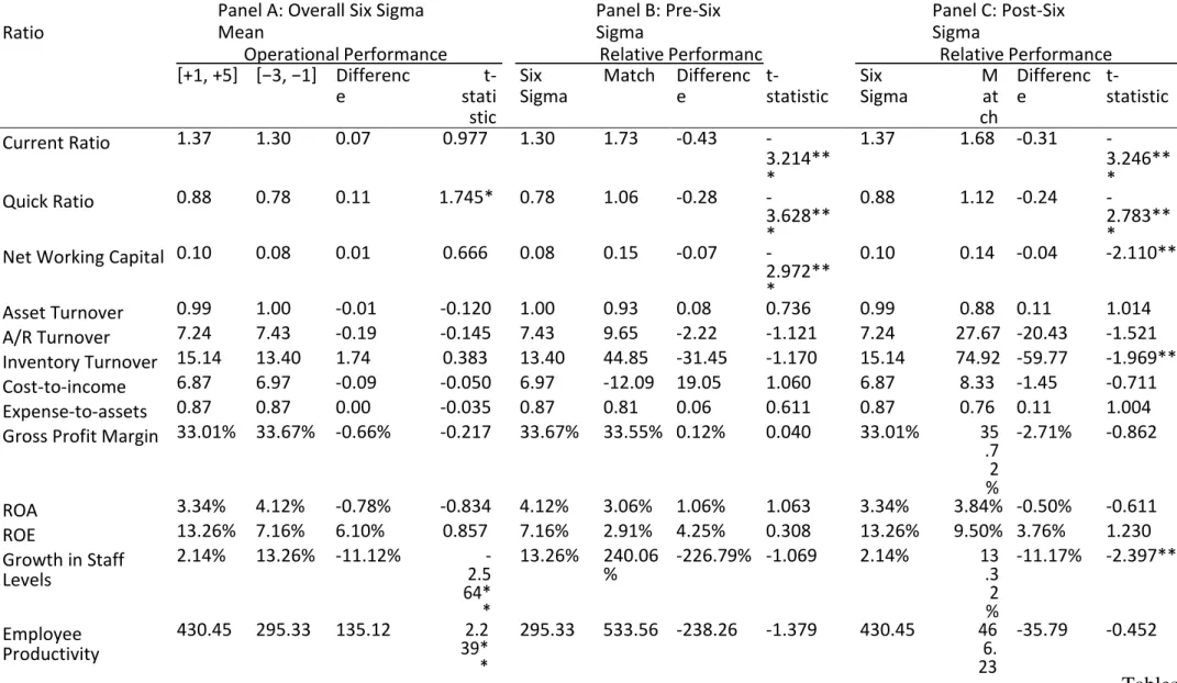
implementation of Six-Sigma processes. 4.2 Robustness Checks
Based on the prior section, our findings are in line with other studies that suggest that labor productivity comes at the price of overworked employees, due to a reduction of staff members (Abernathy, 1978; Tushman and O’Reilly, 1996; Benner and Tushman, 2002, 2003; Naveh and Erez, 2004; Bilgili, et al., 2013). By the same token, we don’t find any supporting evidence of a cost-saving feature of Six-Sigma (as
reported by Dorgan and Dowdy, 2004 or Braunscheidel et al. (2011)), since neither of the expense or cost ratios are statistically better than those for the matching firms.
Partially consistent with Swink and Jacobs (2012), when assessing adjusted performance, we do find mild evidence of a positive long-term effect on ROE post adoption (10% significance at best after year 3), but we fail to find a statistical significantly effect on ROA. The authors find that Six Sigma adoption provides strong evidence of a positive impact on ROA, but the Wilcoxon test reported in this paper suggest that any yearly effect on ROA during the window [−3, +5] is of no statistical significance.
Therefore, we include further tests, as a robustness check. We start by differentiating between two event windows, [−3, −1] and [1,5], to account for full pre- and post-implementation periods rather than yearly performance. We first look at the whole sample and compare the ratios pre- and post-training while also comparing the 108 Six-Sigma companies to the matching 108 companies based on a differences-in-mean-ratios test. Then, we reduce the sample to account for only the eighty-five companies that introduced Six-Sigma at the corporate-wide level. And finally we provide evidence regarding the difference between early and late adoption of Six-Sigma practices, also adjusted for size and industry.