Electrical measurement of cross-sectional position of particles flowing through a microchannel

https://doi.org/10.1007/s10404-018-2055-3 RESEARCH PAPER

Electrical measurement of cross‑sectional position of particles flowing

through a microchannel

Riccardo Reale1 _{· Adele De Ninno}1 _{· Luca Businaro}2 _{· Paolo Bisegna}1 _{· Federica Caselli}1

Received: 15 December 2017 / Accepted: 6 March 2018 © The Author(s) 2018

Abstract

The first high-throughput system for the electrical detection of cross-sectional position and velocity of individual particles flowing through a rectangular microchannel is presented. Lateral position (along channel width) and vertical position (along channel height) are measured using two different sets of coplanar electrodes. In particular, the ratio of travel times measured with electrodes generating a current flow transverse or oblique with respect to particle trajectory yields lateral position. The relative prominence and transit time of a bipolar double-Gaussian signal obtained with a suited electrode configuration, respectively, supply vertical position and velocity. The operating principle is presented by means of finite element numeri-cal simulations. The method is experimentally validated by comparing the electrinumeri-cal estimates of position and velocity of polystyrene beads with optical estimates obtained by processing high-speed images. The system is used to observe bead focusing at different particle Reynolds numbers. This system, providing a fully electrical characterization of single-particle motion, represents a powerful tool, e.g. to understand fluid motion at the microscale, in particle separation studies, or to assess the performance of particle focusing devices. Moreover, it can be simultaneously used to perform single-cell imped-ance spectroscopy, thus achieving an unprecedented multiparamteric characterization.

Keywords Electrical impedance · Microfluidics · Position detection · Coplanar electrodes

1 Introduction

Microfluidic applications are continuing to expand in the fields of nanotechnology, manufacturing and life sciences, and therefore, there is a pressing need for methods to charac-terize fluid behaviour at the microscale and suspended parti-cle motion (Williams et al. 2010; Winer et al. 2014; Tasad-duq et al. 2015). As an example, detecting cross-sectional position of flowing particles is essential in the investigation of self-ordering mechanisms (Gao et al. 2017), inertial parti-cle focusing (Di Carlo 2009) or active particle focusing [e.g.

dielectrophoretic (Shaker et al. 2014) and acustophoretic (Muller et al. 2013)], which have applications in single-cell analysis and sorting (Wyatt Shields IV et al. 2015). In fact, under specific force fields, position can directly indicate the property of target cells (Wang et al. 2017).

Numerous optical methods have been developed to obtain flow field and particle position in microfluidic channels. Conventional video microscopy depicts particle motion projected onto a plane defined by the focus of the objective. For many applications (e.g. micromixers or particle focus-ing devices), visualization of motion in the third dimension is required to fully understand the trajectory of particles (Tasadduq et al. 2015). To that aim, multi-camera (e.g. ste-reoscopic imaging, tomographic imaging) and single camera (e.g. confocal scanning microscopy, anamorphic/astigmatic imaging, digital holographic microscopy, deconvolution and defocusing microscopy) approaches have been proposed [for a description and comparative analysis see e.g. the reviews Lee and Kim (2009), Williams et al. (2010) and Cierpka and Kähler (2012)]. However, those methods require expen-sive and intricate optical setups involving numerous lenses, aperture designs and light sources, or demand for refined Electronic supplementary material The online version of this

article (https ://doi.org/10.1007/s1040 4-018-2055-3) contains supplementary material, which is available to authorized users. * Federica Caselli

caselli@ing.uniroma2.it

1 _{Department of Civil Engineering and Computer Science,}

University of Rome Tor Vergata, 00133 Rome, Italy

2 _{Institute for Photonics and Nanotechnologies, Italian National}

and intensive processing of massive image data (Winer et al. 2014; Lin and Su 2016).

An attractive alternative to optical systems is repre-sented by electrical impedance-based approaches (Wang et  al. 2017; Caselli et  al. 2017; Brazey et  al. 2018). Impedance-based microfluidic devices have been exten-sively studied in the last decade due to their simplicity and potential for low-cost and portable implementation. In par-ticular, microfluidic impedance cytometers for label-free analysis of single particles and cells at high throughput (Cheung et al. 2010; Sun and Morgan 2010; Petchakup et al. 2017) have been used in different biological assays, including particle sizing and counting, cell phenotyping and disease diagnostics [e.g. Haandbæk et al. (2016), McGrath et al. (2017), Rohani et al. (2017), Esfandyar-pour et al. (2017) and Rollo et al. (2017)]. Those systems use electrodes integrated in a microchannel to measure variation in the electric field caused by the transit of par-ticles. The accuracy of the technique is challenged by the positional dependence issue, i.e. identical particles flow-ing in the microchannel along different trajectories pro-vide different signals (Spencer and Morgan 2011). This is due to fringing electric field and may introduce blurring in the estimated particle properties. Compensation strat-egies aimed at solving the positional dependence issue have been proposed by our group, thus achieving high

accuracy particle sizing. To this end, new metrics have been devised, correlating with either lateral (i.e. along channel width) (Caselli et al. 2017, 2018) or vertical (i.e. along channel height) (Spencer et al. 2016; De Ninno et al. 2017) particle position.

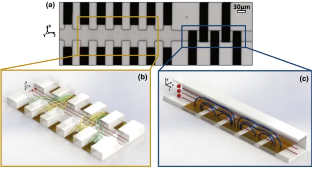
Those metrics are here exploited for quantitative par-ticle localization. The first impedance-based device for high-throughput determination of cross-sectional (i.e. both lateral and vertical) position and velocity of single particles flowing through a rectangular microchannel is presented. The system comprises two consecutive regions, each equipped with a different set of coplanar electrodes (Fig. 1). As detailed in Sect. 2,

(i) an electrical estimate, X, of lateral particle coordi-nate (x-coordicoordi-nate) is obtained from the ratio R of the travel times measured using two sets of electrodes placed in lateral channels (first region, Fig. 1b); (ii) an electrical estimate, Y, of vertical particle

coor-dinate (y-coorcoor-dinate) is obtained from the relative prominence P (De Ninno et al. 2017) of a bipolar double-Gaussian impedance signal recorded using five electrodes spanning the width of the main chan-nel (second region, Fig. 1c);

(a) x

z y

30 m

LATERAL POSITION DETERMINATION VERTICAL POSITION AND VELOCITY DETERMINATION

(c) (b)

Fig. 1 a Microscope image of the electrical sensing area. The region highlighted with a yellow box, comprising five pairs of lateral elec-trodes, is used for the determination of particle lateral position. The region highlighted with a blue box, formed by five electrodes span-ning the channel width, is used for the determination of particle verti-cal position and velocity. b, c 3D rendered models of the two

meas-uring regions. Lateral position is determined by comparing signals relevant to transverse and oblique current flows (yellow and green field lines in panel (b), respectively). Vertical position and velocity are determined exploiting an electrode configuration that generates a peculiar current distribution (blue field lines), characterized by alter-nating high- and low-field regions (colour figure online)

(iii) particle velocity is extracted from the latter signal, dividing the spatial length of the sensing zone by the transit time.

A thorough validation of the proposed approach is reported. Impedance signals for 6- and 10-μ m polystyrene beads have been collected. The electrical estimates of parti-cle cross-sectional position and velocity are compared with the estimates derived by image processing of optical frames recorded using a high-speed camera. Moreover, the method is used to monitor the bead flow under different flow rates, and partial inertial focusing is observed.

The paper is organized as follows: the operating principle enabling the electrical estimate of particle cross-sectional position and velocity is presented in Sect. 2, the experi-mental methods are described in Sect. 3, and validation and results are presented in Sect. 4. Finally, conclusions are drawn.

2 Operating principle

2.1 Electrical estimate of particle lateral position The chip region used for the electrical estimation of particle lateral position (i.e. x-coordinate) exploits the concept of liquid electrodes (Demierre et al. 2007). They are vertical equipotential surfaces generated on apertures of the main channel walls by recessed coplanar electrodes patterned at the bottom of dead-end lateral chambers (Fig. 1b). Liquid electrodes provide a nearly homogeneous electric field over the total channel height while keeping a simple process flow with a single planar metal layer (Mernier et al. 2012).

In the present work, five pairs of coplanar electrodes are considered and the following wiring scheme is proposed (Fig. 2a): an AC voltage is applied to two stimulation elec-trodes on one side of the main channel (the 2nd and the 4th electrodes along z, at x > 0 ), and two differential current signals are measured using four sensing electrodes located on the opposite side (i.e. at x < 0 ). The first signal, denoted

I_TSV , is the difference in electric current flowing through

the sensing electrodes with the same z-coordinate as the stimulation electrodes (the 2nd and the 4th electrodes along

z) which features a current path transverse to particle flow.

The second signal, denoted IOBQ , is the difference in

elec-tric current flowing through two sensing electrodes with a

z-coordinate different from the stimulating electrodes (the

1st and the 5th electrodes along z) featuring a current path oblique with respect to particle flow. An analogous wiring scheme was introduced in Spencer et al. (2016) for a chip comprising five pairs of facing electrodes, aimed at solving the positional dependence issue.

1 2 (a) (b) (c) ITSV IOBQ V -+ + -1 2 x z y (d)

Fig. 2 _{Electrical metric encoding particle lateral position. a Diagram} showing the electrode design and the wiring scheme. Two differen-tial current measurements are taken: a transverse measurement ( ITSV )

and an oblique measurement ( IOBQ ). b, c FEM simulations of the

dif-ferential current signals (real part) generated by a flowing particle (6-μm-diameter insulating bead). b When a particle travels near the stimulation electrodes (i.e. in the positive x region, trajectory 1) the peak-to-peak distances ΔzTSV and ΔzOBQ are similar and their ratio is

close to one. c When a particle travels near the measuring electrodes (i.e. in the negative x region, trajectory 2) ΔzOBQ is greater than ΔzTSV

and their ratio is greater than one. d Simulated peak-to-peak time ratio R (equivalent to ΔzOBQ∕ΔzTSV ) versus particle x-coordinate. The

one-to-one relationship between R and x shows that the ratio R can be used to estimate particle lateral position

Figure 2b [resp. c] shows the trace (real part) obtained in simulation when a dielectric bead travels along trajectory 1 [resp. 2] depicted in Fig. 2a. The differential signals ITSV and I_OBQ exhibit a bipolar profile, and the relevant peak-to-peak

distances are denoted by ΔzTSV and ΔzOBQ , respectively.

While ΔzTSV is the same for both trajectories, ΔzOBQ depends

on particle lateral position: it is higher for particles travelling near the sensing electrodes (trajectory 2, Fig. 2c) than for particles travelling near the stimulation electrodes (trajectory 1, Fig. 2b). From the experimental point of view, the peak-to-peak times ΔtTSV and ΔtOBQ are available, instead of the

peak-to-peak distances ΔzTSV and ΔzOBQ . Although ΔtTSV

and ΔtOBQ depend on particle velocity, their ratio

coinciding with ΔzOBQ∕ΔzTSV , is a dimensionless quantity,

independent of velocity, that correlates with particle lateral position. Consequently, R can be used to obtain an electrical estimate X of particle x-coordinate.

A simple geometric argument, assuming straight current paths (Fig. 2a), yields the following linear estimate:

where W denotes the channel width. Simulation results (Fig. 2d) confirm that such a simple model is valid, except for a slight saturation at extremal lateral positions. A refined model, involving quadratic and cubic corrections, is intro-duced to cover the whole position range:

The calibration procedure of the parameters b1 and b2 is

described in Sect. 4.3.

2.2 Electrical estimate of particle vertical position and particle velocity

In order to estimate particle vertical position (i.e. y-coor-dinate), the sensing zone comprising five electrodes span-ning the main channel width (Fig. 1c) is used. The relevant wiring scheme, introduced in De Ninno et al. (2017), is depicted in Fig. 3a: an AC voltage signal is applied to the central electrode, and the difference in electric current flow-ing through the lateral electrodes is measured. Intermediate electrodes are left floating. This wiring scheme results in a non-homogeneous electric field distribution along the chan-nel axis (z-direction), characterized by weak-field regions in front of the floating electrodes, which in turn are reflected as local minima in the collected current. Therefore, the result-ing signal trace exhibits a bipolar double-Gaussian (BDG) profile and is denoted as IBDG.

(1) R= Δt_OBQ∕Δt_TSV, (2) X_lin= W ( 3 2− R ) , (3) X= W(3 2− R )[ 1+ b₁(3 2− R ) + b₂(3 2 − R )2] . 1 2 1 2 FL V FL IBDG -+ x z y (a) (b) (c) (d)

Fig. 3 Electrical metric encoding particle vertical position. a Diagram show-ing the electrode design and the wirshow-ing scheme. Compared to the standard three-electrode measurement configuration [e.g. Gawad et  al. (2001)], two additional floating electrodes are inserted between the stimulation and the measuring electrodes. These electrodes create a non-homogeneous electric field distribution, shunting particles travelling close to them. b, c FEM simula-tions of the differential current signal (real part) generated by a flowing particle (6-μm-diameter insulating bead). The signal exhibits bipolar double-Gaussian (BDG) shape which is characterized by the relative prominence P of the peaks compared to the saddle. b When a particle travels far from the electrodes (i.e. in the positive y region, trajectory 1) the relative prominence P is low. c When a particle travels near the electrodes (i.e. in the negative y region, trajectory 2) the relative prominence P is high. d Simulated relative prominence P versus particle y-coordinate. The one-to-one relationship between P and y shows that the relative prominence P can be used to estimate particle vertical position

Figure 3b [resp. c] shows the trace (real part) obtained in simulation when a dielectric bead travels along trajec-tory 1 [resp. 2] depicted in Fig. 3a. The prominence of the two peaks with respect to the saddle in between is higher for particles travelling close to the electrodes (trajectory 2, Fig. 3c) than for particles travelling away from the elec-trodes (trajectory 1, Fig. 3b). Because signal amplitude also depends on particle size, the following normalized metric, referred to as relative prominence, was introduced in De Ninno et al. (2017):

where m and M are the signal amplitude at the saddle and peaks, respectively.

Finite element simulations (Fig. 3d) show that the rela-tive prominence P correlates with the height of particle tra-jectory (y-coordinate): the higher the former, the lower the latter. This claim has been experimentally supported in De Ninno et al. (2017) by means of a quantitative defocusing approach (Wu et al. 2005). As a consequence, the relative prominence P can be used to obtain an electrical estimate Y of particle y-coordinate. In particular, a quadratic model is used in this work:

where H denotes channel height. As shown in Caselli and Bisegna (2017), the parameters ci depend on the experimen-tal setup (e.g. buffer conductivity, frequency of the AC stim-ulation, electrode double-layer capacitance). The relevant calibration procedure is described in Sect. 4.3.

An electrical estimate V of particle velocity is obtained from the signal IBDG as follows:

where ΔzBDG is the distance between the centres of the

float-ing electrodes ( ΔzBDG= 80 μ m for the present geometry)

and ΔtBDG is the relevant transit time (De Ninno et al. 2017).

3 Experimental

The impedance chip consists of a glass microscope slide with integrated gold microelectrodes, bonded to a PDMS-embedded microchannel (Fig. 1). The device was fabricated following standard microfabrication techniques, as reported elsewhere (De Ninno et al. 2017). The main channel was 40 μ m wide and 21.5 μ m high. The lateral channels in the lateral position determination region were 30 μ m wide and 30 μ m apart from each other, with electrodes recessed by 20  μ m with respect to the main channel. The five electrodes (4) P= M− m M , (5) Y = H (c₀+ c₁P+ c₂P2), (6) V = Δz_BDG∕Δt_BDG,

in the vertical position determination region, spanning the main channel width, were 30 μ m wide with a 10-μ m gap between them. For fluidic access, Teflon tubing (OD: 1/16″) was inserted into chip inlet and connected to a 500-μ l glass syringe (Hamilton) loaded on a syringe pump (Elite 11, Har-vard Apparatus). The chip was connected electrically to a custom chip holder using pogo pins.

3.2 Sample preparation

The system was tested using polystyrene beads with diam-eters of 6 or 10 μ m (Sigma-Aldrich). The beads were re-suspended to a concentration of approximately 106 beads/

ml in PBS containing 0.1% Tween 20 and enough sucrose to match particle density (1050 kg/m3 ). The conductivity of

the final medium was 1.1 S/m. The samples were sonicated prior to the experiments, in order to prevent bead aggrega-tion. Samples were pumped through the device at a flow rate of 3, 10 or 30 μl/min.

3.3 Impedance data acquisition and processing Electrical signals were measured using two transimpedance amplifiers (HF2TA, Zurich Instruments) and an impedance spectroscope (HF2IS, Zurich Instruments). Details of the electrical connections are reported in Supplementary mate-rial, Figure S1. Excitation signals of 8 V, 1 MHz and 6 V, 884.8 kHz were used for the determination of lateral and vertical positions, respectively. Differential currents were sampled at 115.2 kSa/s, with 6, 20 or 60 kHz filter band-width, respectively, for 3, 10 or 30 μl/min flow rate.

Event detection in the data streams was performed with a previously reported algorithm (Caselli and Bisegna 2016), and a simple MATLAB script was used for event feature extraction by template fitting (Spencer et al. 2016; De Ninno et al. 2017). In particular, for each detected event the ratio

R (Eq. 1) was computed from the peak-to-peak times of the

oblique and transverse signals IOBQ and ITSV , whereas the

relative prominence P (Eq. 4) and the transit time ΔtBDG

were extracted from the bipolar double-Gaussian signal

I_BDG . Parameters R , P and Δt_BDG were then used to

com-pute electrical position X, electrical height Y and electrical velocity V by means of Eqs. (3), (5) and (6), respectively. 3.4 Optical data acquisition and processing

For validation purposes, independent estimates of parti-cle cross-sectional position and velocity were obtained by means of an optical approach. The optical recording region was located downstream the electrical sensing region. Images of a 1024 × 112 pixels area around the channel were recorded using a high-speed camera (Photron FASTCAM Mini UX100, 4000 fps, 4 μ s shutter time) mounted on an

inverted microscope (Zeiss Axio Observer, 20× objec-tive). Images were first saved on the camera local memory (10.6 GB) and then moved to a desktop computer. These settings allowed for a continuous optical recording of 25 s.

In order to ease the image segmentation step (i.e. the identification of beads in the recorded frames), the elec-trical velocity V of each event detected in the impedance data streams was used to predict particle entrance time in the optical region, thus reducing the computational cost of image processing. For each particle, the optical lateral posi-tion Xopt was computed as the distance between the particle

centre and the channel z-axis (Fig. 4a), whereas the optical velocity Vopt was computed as the product of the distance

travelled by the particle across two consecutive frames and the camera frame rate (Fig. 4b). The optical vertical position

Y_opt (Fig. 4c) was obtained by using a quantitative

defocus-ing approach (Wu et al. 2005; Winer et al. 2014) based on

calibration data relating the y-position of a particle to its observed central intensity (De Ninno et al. 2017).

3.5 Particle inertial focusing

The onset of particle focusing can be observed in the lami-nar regime, when inertial effects start to become relevant. It can be predicted by particle Reynolds number, defined for a rectangular channel as (Di Carlo et al. 2007):

where Re is channel Reynolds number, a is particle diam-eter, U is fluid maximum velocity, Dh is cannel hydraulic diameter (defined as 2 WH∕(W + H) ) and μ and 𝜌 are fluid dynamic viscosity and density, respectively.

At Rep≥1 , randomly dispersed particles in a

rectan-gular microchannel tend to order in specific equilibrium positions. They first migrate from the channel bulk towards equilibrium positions near the walls (fast migration), and then, they migrate parallel to channel walls into wall-centred equilibrium positions (slow migration) (Zhou and Papautsky 2013). In a square channel, there are four stable position in correspondence with the middle of each wall, whereas in a rectangular channel the positions close to the short walls become unstable and only two equilibrium position are left (Zhou and Papautsky 2013; Amini et al. 2014).

4 Results

4.1 Information provided by the electrical metrics R and P

Figure 5 shows the density plot for 6-μm-diameter beads pumped at 3 μl/min, with the relative prominence P plotted against the peak-to-peak time ratio R. The particle Reynolds number Rep , equal to 0.11, implies that little inertial focusing

is established, so that particles adopt a random distribution in the rectangular channel cross section. Since a one-to-one monotonic decreasing relationship prevails between R and x [resp. P and y], topological information on particle position in the cross section is provided by the (R, P) density plot. In particular, particles are expected to visit a rectangular region, as experimentally confirmed.

Examples of experimental single-particle impedance sig-nals are shown in Fig. 5, along with arrows indicating the position of the particle on the density plot. Particles (i), (ii), (iv) and (v) have trajectories near the corners of the cross section. As an example, particle (i) flows near the lower-left channel corner, because its signal exhibits high relative prominence P (i.e. low y-coordinate) and high peak-to-peak (7) Re_p= Re ( a Dh )2 = 𝜌Ua 2 μDh

(a) LATERAL POSITION

x z x z x z (b) VELOCITY x z x z (c) VERTICAL POSITION 15 m 15 m 15 m 15 m 15 m 15 m 15 m 15 m

Fig. 4 _{Optical estimate of particle position and velocity. The optical} recording region is located downstream the electrical sensing region. The dark area on the left in panels (a) and (b) is part of the rightmost electrode shown in Fig. 1a. a Lateral position Xopt is determined by

measuring the distance between particle centre and channel z-axis. b Velocity Vopt is determined by measuring the distance travelled by a

particle along the z-axis between two consecutive frames and multi-plying it by the camera frame rate (1∕Δt) . c Vertical position Yopt is

determined by measuring particle central intensity and referring to a quantitative defocusing calibration set

time ratio R (i.e. low x-coordinate). Particle (iii), exhibiting intermediate values of R and P and shortest ΔtBDG (i.e.

high-est velocity), flows along the channel axis. 4.2 Inertial focusing detection

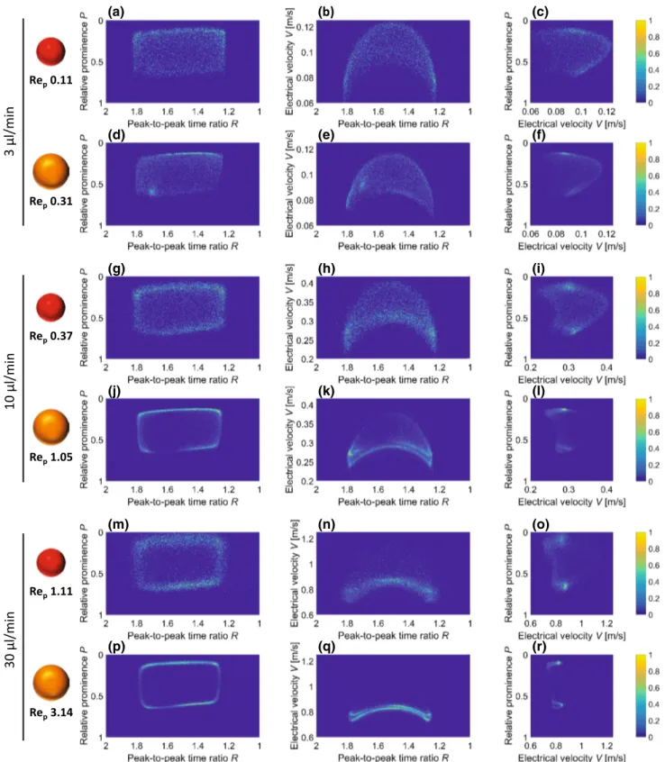
The topological information provided by the electrical metrics R and P, along with the electrical velocity V, was used to investigate inertial focusing effects. To this aim, different degrees of focusing were obtained experimentally by varying flow rate and beads diameter, thus varying Rep .

In particular, Rep values from 0.11 (6-μm-diameter beads,

3 μl/min) to 3.14 (10-μm-diameter beads, 30 μl/min) were considered (Fig. 6).

As shown in the (R, P) plane, at Rep= 0.11 particles

were randomly distributed in the cross section (Fig. 6a). By increasing Rep , particles migrated away from the

chan-nel centre towards lines parallel to the four chanchan-nel walls (Fig. 6, first column). The higher the particle Reynolds number Rep , the more pronounced the hydrodynamic

focusing. This effect was analysed on the (R, V) plane as well (Fig. 6, second column): at low Rep , the complete

parabolic velocity profile could be observed, whereas when Rep was increased, the high-velocities region

(rel-evant to particles travelling close to the channel centre) became progressively less populated and visited by fewer particles. At Rep= 3.14 , the parabolic velocity profile

collapsed to the zones corresponding to velocities of the preferential positions parallel to channel walls. The same behaviour could be observed on the (P, V) plane (Fig. 6, third column).

At all values of Rep , the ranges of R and P values visited by

the 10-μm-diameter beads were slightly narrower than those of the 6-μm-diameter beads, since a narrower cross section is available to the centres of the former particles, due to their larger size. Moreover, compared to 6-μ m beads, 10-μ m beads showed more pronounced focusing when operated under the same hydrodynamic conditions (i.e. same Rep ). This might

be explained considering that for 10-μ m beads the ratio of bead diameter to channel hydraulic diameter, a∕Dh , is close to 0.4 and additional steric effects become relevant (Amini et al. 2014).

4.3 Calibration procedure used to map the (R, P)‑plane onto the (X, Y)‑plane

In order to transform the electrical metrics (R and P) into electrical estimates (X and Y) of the Cartesian coordinates of particle centre (x and y), model Eqs. (3) and (5) were used. The relevant model parameters were calibrated using the experiment at Rep= 0.11 (6-μm-diameter beads at 3 μ

l/min flow rate), where particles adopt a random distribu-tion in the channel cross secdistribu-tion (Fig. 6a–c). In particular,

(iii)

(i)

(iv)

(iii)

(v)

(i)

(ii)

(iv)

(v)

(ii)

Fig. 5 _{Density plot for 6-μm-diameter beads (flow rate 3 μl/min), with} the relative prominence P plotted against the peak-to-peak time ratio

R. i–v Are experimental single-particle signals for the data points in

the density plot ( ITSV : orange line; IOBQ : green line; IBDG : blue line).

Fitting templates are also shown (grey lines). The histogram of the root-mean-square error of the fit, normalized by peak amplitude, is reported in Supplementary material, Figure S2 (colour figure online)

3 l/mi n 10 l/mi n 30 l/mi n (a) Rep0.11 Rep0.31 (b) (c) (d) (e) (f) (g) (h) (i) (j) (k) (l) (m) (n) (o) (p) (q) (r) Rep0.37 Rep1.05 Rep1.11 Rep3.14

Fig. 6 Density plots of relative prominence P versus peak-to-peak time ratio R (first column); electrical velocity V versus peak-to-peak time ratio R (second column); electrical velocity V versus relative prominence P (third column). Six-μm-diameter beads (odd rows) or 10-μm-diameter beads (even rows) were pumped through the device

at flow rates of a–f 3 μl/min, g–l 10 μl/min, and m–r 30 μl/min. The higher the particle Reynolds number Rep , the more pronounced the

hydrodynamic focusing. At least 6500 events are reported in each density plot and colour-bar values are normalized with respect to the highest bin count (colour figure online)

accounting for finite particle diameter a = 6 μ m, and allow-ing for a small gap, g ≈ 2 μ m, between particle boundary and channel walls, particle centre coordinates satisfy the following inequalities:

where s = (a∕2) + g . Accordingly, parameters b1 and b2

appearing in Eq. (3) were determined by imposing the conditions:

where RL and RH are the 1 and 99% percentile values of R,

respectively (Fig. 7a, red lines). Their values are reported in Table 1, along with the resulting calibration coefficients

b₁ and b₂.

An analogous procedure was used to calibrate parameters

c₀ , c₁ and c₂ appearing in Eq. (5). However, an additional

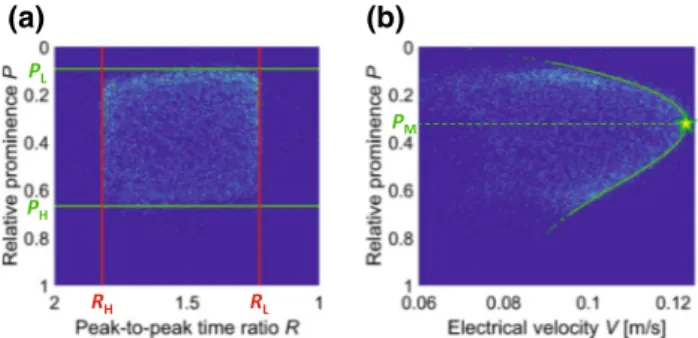
con-dition was needed in this case. Figure 7b shows the density plot of the electrical velocity V versus the relative prominence P. The curve Vmax(P) that gives the maximum velocity V

meas-ured at each relative prominence value P is also plotted (green curve). It was computed using cubic 95% quantile regression instead of maxima search, in order to obtain a robust algorithm against outliers. Because, for any y, the maximum particle velocity in the channel cross section is attained at x = 0 , and a one-to-one correspondence between y and P prevails, the curve

V_max(P) represents the velocity profile on the line x = 0 , as a function of P. That curve attains its maximum value at a rela-tive prominence value PM which corresponds to y = 0 , since

the maximum velocity is attained at channel centre.

(8) |x| ≤W 2 − s , |y| ≤ H 2 − s, (9) X(R_L) = W 2 − s, X(RH) = − W 2 + s,

Therefore, the parameters c0 , c1 , c2 entering Equation (5)

were determined by imposing the conditions:

where PL and PH are the 1 and 99% percentile values of P,

respectively (Fig. 7a, green lines). The values of PL , PM and P_H are reported in Table 2, along with the resulting

calibra-tion coefficients c0 , c1 and c2.

4.4 Optical validation of electrical position (X, Y) and electrical velocity V

The electrical estimates of particle lateral position X (Eq. 3), vertical position Y (Eq. 5) and velocity V (Eq. 6) were com-pared with the optical estimates Xopt , Yopt and Vopt in Fig. 8

(6-μ m beads, 10 μl/min flow rate).

The density plot of the electrical lateral position X against the optical lateral position Xopt shows a very good

agree-ment between the two estimates along the whole position range (Fig. 8a, 0.97 correlation coefficient, 2.2 μ m root-mean-square difference, that is 5.6% of channel width). It is pointed out that even the very simple estimate Xlin proposed

in Eq. (2), based on a geometric argument and not requiring any calibration, provides a reasonably accurate estimate of particle lateral position as shown by the density plot of Xlin

versus Xopt (Supplementary material, Figure S4).

A reasonable agreement is found between the electrical vertical position Y and the optical one Yopt (Fig. 8b, 0.94

cor-relation coefficient, 1.7 μ m root-mean-square difference, that is 8.1% of channel height). As a matter of fact, the procedure used to estimate the lateral position Xopt , which is based on

bead segmentation within image frames, is more accurate than the procedure used to estimate the vertical position

Y_opt , which uses a calibration-based defocusing approach

(De Ninno et al. 2017). Moreover, the electrical estimate of the vertical position Y, based on the relative prominence P, may exhibit some blurring due to fitting inaccuracy at low relative prominence values (corresponding to high Y values). It is noticed that the electrical method used for the lateral (10) Y(P_L) = H 2 − s, Y(PH) = − H 2 + s, Y(PM) = 0, (b) (a) R_H R_L P_L PH PM

Fig. 7 Calibration experiment (6-μ m beads, 3  μl/min flow rate,

Re_p= 0.11 ). a Density plot of relative prominence P versus peak-to-peak time ratio R. The 1 and 99% percentile values of R (red lines) and P (green lines) are shown. The corresponding values are labelled as RL , RH (Table 1), and PL , PH (Table 2). See also Supplementary

material, Figure S3. b Density plot of electrical velocity V versus rel-ative prominence P. The cubic 95% quantile regression is shown in green. The relative prominence value PM corresponding to the

maxi-mum velocity Vmax= 0.12 m/s is visualized (Table 2). Colour-bar

values are normalized with respect to the highest bin count (colour figure online)

Table 1 Values of 1 and 99% percentile of R (Fig. 7a) and resulting calibration parameters (Eq. 3)

RL RH b1 b2

1.22 1.82 0.48 3.14

Table 2 _{Values of 1 and 99% percentile of P (Fig. 7a) and value of}

P at maximum velocity (Fig. 7b). Resulting calibration parameters

(Eq. 5)

PL PM PH c0 c1 c2

position determination could be replicated in a vertical con-figuration using five pairs of facing electrodes (Spencer et al. 2016), thus providing an even more accurate estimate of particle vertical position, at the expense of a more complex microfabrication process.

The density plot of the electrical velocity V against the optical velocity Vopt is shown in Fig. 8c. An excellent

agree-ment is found between the two measureagree-ments (0.97 correla-tion coefficient, 0.01 m/s root-mean-square difference, that is 2.3% of maximum particle velocity). The velocity range measured optically and electrically is (0.20–0.39) m/s, with average particle velocity of 0.30 m/s. By comparison, the velocity distribution in steady state, hydrodynamically fully developed, laminar flow for Newtonian fluids in rectangular channels (Spiga and Morini 1994) has maximum 0.39 m/s and average 0.19 m/s for the present channel cross section and flow rate. In fact, particles tend to avoid trajectories very close to the channel walls, so that their average velocity is greater than average fluid velocity.

4.5 Quantitative particle positioning within the channel cross section

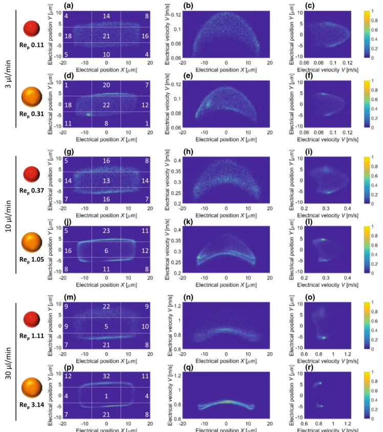
The R ↦ X and P ↦ Y mappings (namely Eqs. 3 and 5 with the coefficient values reported in Tables 1 and 2) were applied to the data sets considered in Fig. 6. The resulting (X, Y), (X, V) and (Y, V) density plots are shown in Fig. 9. For each experimental condition, the percentage of particles falling in each bin of a 3 × 3 regular grid in the (X, Y) plane (Fig. 9, first column) is also indicated (bin size W∕3 × H∕3).

At Rep= 0.11 , when particles are randomly distributed,

21% of the particles visited the central bin and lower per-centages were found in the other bins (especially the corner

bins), due to a minimum distance of particle centres from channel walls imposed by finite particle size. By increasing

Re_p , the particles moved away from the central bin towards

peripheral bins. At Rep = 3.14 , only 1% of the particles

vis-ited the central bin, and the highest particle concentration was found in the bin corresponding to the centre of the long walls, in agreement with the literature (Zhou and Papaut-sky 2013; Amini et al. 2014) (see Supplementary material, Figure S5).

The evolution of particle distribution in the channel cross section as Rep increases is reflected in changes of the

veloc-ity profiles observed in the (X, V) and (Y, V) planes (Fig. 9, second and third column, respectively).

5 Conclusion

In this work, we reported the first high-throughput electrical system for the measurement of cross-sectional position and velocity of single particles flowing through a microchan-nel. Lateral position was computed measuring the ratio of oblique and transverse transit times, whereas vertical posi-tion and velocity were extracted from the relative promi-nence and transit time of a bipolar double-Gaussian signal measured with a suited wiring scheme. Transit-time ratios and relative prominence values supplied valuable topo-logical information on particle position in the microchan-nel cross section. Moreover, they could be transformed to quantitative estimates of lateral and vertical positions using a simple calibration procedure. Optical validation confirmed the soundness of the proposed approach. As an applicative example, the effects of particle size and flow rate on inertial particle focusing were investigated.

Fig. 8 Comparison between electrical estimates X,  Y,  V and optical estimates Xopt, Yopt, Vopt (6-μ m beads, 10 μl/min flow rate). Data are

shown as density plots (2500 events), and the bisector line is dashed in red. Colour-bar values are normalized with respect to the highest bin count. a Electrical lateral position X (Eq. 3) versus optical lateral position Xopt (0.97 correlation coefficient, 2.2 μ m root-mean-square

difference, that is 5.6% of channel width). b Electrical vertical posi-tion Y (Eq. 5) versus optical vertical position Yopt (0.94 correlation

coefficient, 1.7 μ m root-mean-square difference, that is 8.1% of chan-nel height). c Electrical velocity V (Eq. 6) versus optical velocity Vopt

(0.97 correlation coefficient, 0.01  m/s root-mean-square difference, that is 2.3% of maximum particle velocity) (colour figure online)

3 l/mi n 10 l/mi n 30 l/mi n (a) Rep0.11 Rep0.31 (b) (c) (d) (e) (f) (g) (h) (i) (j) (k) (l) (m) (n) (o) (p) (q) (r) Rep0.37 Rep1.05 Rep1.11 Rep3.14 12 11 4 7 32 1 21 4 8 5 11 16 8 23 6 11 12 8 1 7 18 11 20 22 8 12 1 5 8 14 7 16 13 16 14 7 9 9 9 7 22 5 21 10 8 4 8 18 5 14 21 10 16 4

Fig. 9 Effect of particle Reynolds number Rep on particle focusing.

Measurements of 6-μ m (odd rows) or 10-μm-diameter (even rows) beads, pumped through the device at 3 μl/min (a–f), 10 μl/min (g–l) or 30 μl/min (m–r) flow rate, are shown. For each experimental con-dition, density plots of electrical position Y versus electrical posi-tion X (first column), electrical velocity V versus electrical posiposi-tion

X (second column), electrical velocity V versus electrical position Y

(third column) are reported. In the (X, Y) density plot (first column), the percentage of particles falling in each bin of a 3 × 3 grid (white dotted lines) is also indicated. The higher the particle Reynolds num-ber Rep , the more pronounced the hydrodynamic focusing. At least

6500 events are reported in each density plot and colour-bar values are normalized with respect to the highest bin count (colour figure online)

The method has been demonstrated with reference to spherical beads. It applies as well to spherical cells, whose behaviour at low frequency (i.e. below the range of the 𝛽 -dispersion) is similar to that of an insulating particle (e.g. Schade-Kampmann et al. (2008), Haandbaek et al. (2014)). The method is also promising for nonspherical particles or cells because, although the latter yield impedance signals depending on their orientation (Jones 1995; Fernandez et al. 2017), the transit times and the relative prominence are not significantly affected by particle orientation.

This fully electrical label-free approach to particle moni-toring, implemented with a simple coplanar chip layout and based on current signals instead of massive image data, rep-resents an effective tool for investigating the behaviour of flowing particles at the microscale. Moreover, the device can be simultaneously used to perform single-cell impedance spectroscopy, thus achieving a multi-parametric characteri-zation embracing size, membrane properties and intracellu-lar conductivity in addition to particle position and velocity. Acknowledgements _{This work was supported by the Scientific} Inde-pendence of Young Researchers Programme (SIR 2014) under Grant RBSI14TX20-MUSIC “Multidimensional Single-Cell Microfluidic Impedance Cytometry”.

Open Access This article is distributed under the terms of the Crea-tive Commons Attribution 4.0 International License (http://creat iveco mmons .org/licen ses/by/4.0/), which permits unrestricted use, distribu-tion, and reproduction in any medium, provided you give appropriate credit to the original author(s) and the source, provide a link to the Creative Commons license, and indicate if changes were made.

References

Amini H, Lee W, Di Carlo D (2014) Inertial microfluidic physics. Lab Chip 14:2739. https ://doi.org/10.1039/C4LC0 0128A

Brazey B, Cottet J, Bolopion A, Van Lintel H, Renaud P, Gauthier M (2018) Impedance-based real-time position sensor for lab-on-a-chip devices. Lab Chip 18(5):818. https ://doi.org/10.1039/C7LC0 1344B

Caselli F, Bisegna P (2016) A simple and robust event-detection algo-rithm for single-cell impedance cytometry. IEEE Trans Biomed Eng 63(2):415. https ://doi.org/10.1109/TBME.2015.24622 92

Caselli F, Bisegna P (2017) Simulation and performance analysis of a novel high-accuracy sheathless microfluidic impedance cytometer with coplanar electrode layout. Med Eng Phys 48:81. https ://doi. org/10.1016/j.meden gphy.2017.04.005

Caselli F, De Ninno A, Reale R, Businaro L, Bisegna P (2018) A novel wiring scheme for standard chips enabling high-accuracy imped-ance cytometry. Sens Actuators B Chem 256:580. https ://doi. org/10.1016/j.snb.2017.10.113

Caselli F, Reale R, Nodargi NA, Bisegna P (2017) Numerical inves-tigation of a novel wiring scheme enabling simple and accurate impedance cytometry. Micromachines 8(9):283. https ://doi. org/10.3390/mi809 0283

Caselli F, Reale R, De Ninno A, Errico V, Businaro L, Bisegna P (2017) 3D particle localization in a microfluidic impedance

cytometer. In: 21th international conference on miniaturized sys-tems for chemistry and life sciences, MicroTAS

Cheung KC, Di Berardino M, Schade-Kampmann G, Hebeisen M, Pierzchalski A, Bocsi J, Mittag A, Tárnok A (2010) Microfluidic impedance-based flow cytometry. Cytom Part A 77(7):648. https ://doi.org/10.1002/cyto.a.20910

Cierpka C, Kähler CJ (2012) Particle imaging techniques for volumet-ric three-component (3D3C) velocity measurements in microflu-idics. J Vis 15(1):1. https ://doi.org/10.1007/s1265 0-011-0107-9

Di Carlo D (2009) Inertial microfluidics. Lab Chip 9:3038. https ://doi. org/10.1039/B9125 47G

Di Carlo D, Irimia D, Tompkins RG, Toner M (2007) Continuous iner-tial focusing, ordering, and separation of particles in microchan-nels. Proc Natl Acad Sci USA 104:18892. https ://doi.org/10.1073/ pnas.07049 58104

De Ninno A, Errico V, Bertani FR, Businaro L, Bisegna P, Caselli F (2017) Coplanar electrode microfluidic chip enabling accurate sheathless impedance cytometry. Lab Chip 17:1158. https ://doi. org/10.1039/C6LC0 1516F

Demierre N, Braschler T, Linderholm P, Seger U, van Lintel H, Renaud P (2007) Characterization and optimization of liquid electrodes for lateral dielectrophoresis. Lab Chip 7:355. https ://doi.org/10.1039/ B6128 66A

Esfandyarpour R, DiDonato MJ, Yang Y, Durmus NG, Harris JS, Davis RW (2017) Multifunctional, inexpensive, and reusable nanoparticle-printed biochip for cell manipulation and diagnosis. Proc Natl Acad Sci USA 114(8):E1306. https ://doi.org/10.1073/ pnas.16213 18114

Fernandez RE, Rohani A, Farmehini V, Swami NS (2017) Review: microbial analysis in dielectrophoretic microfluidic systems. Anal Chim Acta 966:11. https ://doi.org/10.1016/j.aca.2017.02.024

Gao Y, Magaud P, Baldas L, Lafforgue C, Abbas M, Colin S (2017) Self-ordered particle trains in inertial microchannel flows. Microfluid Nanofluid 21(10):154. https ://doi.org/10.1007/s1040 4-017-1993-5

Gawad S, Schild L, Renaud P (2001) Micromachined impedance spec-troscopy flow cytometer for cell analysis and particle sizing. Lab Chip 1(1):76. https ://doi.org/10.1039/B1039 33B

Haandbaek N, Bürgel SC, Heer F, Hierlemann A (2014) Characteriza-tion of subcellular morphology of single yeast cells using high frequency microfluidic impedance cytometer. Lab Chip 14(2):369.

https ://doi.org/10.1039/C3LC5 0866H

Haandbæk N, Bürgel SC, Rudolf F, Heer F, Hierlemann A (2016) Char-acterization of single yeast cell phenotypes using microfluidic impedance cytometry and optical imaging. ACS Sens 1(8):1020.

https ://doi.org/10.1021/acsse nsors .6b002 86

Jones TB (1995) Electromechanics of particles. Cambridge University Press, Cambridge

Lee SJ, Kim S (2009) Advanced particle-based velocimetry techniques for microscale flows. Microfluid Nanofluid 6(5):577. https ://doi. org/10.1007/s1040 4-009-0409-6

Lin CH, Su SY (2016) Depth position detection for fast moving objects in sealed microchannel utilizing chromatic aberration. Biomicro-fluidics 10(1):011904. https ://doi.org/10.1063/1.49399 43

McGrath JS, Honrado C, Spencer D, Horton B, Bridle HL, Morgan H (2017) Analysis of parasitic protozoa at the single-cell level using microfluidic impedance cytometry. Sci Rep 7:2601. https ://doi. org/10.1038/s4159 8-017-02715 -y

Mernier G, Duqi E, Renaud P (2012) Characterization of a novel impedance cytometer design and its integration with lateral focusing by dielectrophoresis. Lab Chip 12(21):4344. https ://doi. org/10.1039/c2lc4 0551b

Muller PB, Rossi M, Marín AG, Barnkob R, Augustsson P, Laurell T, Kähler CJ, Bruus H (2013) Ultrasound-induced acoustopho-retic motion of microparticles in three dimensions. Phys Rev E 88:023006. https ://doi.org/10.1103/PhysR evE.88.02300 6

Petchakup C, Li KHH, Hou HW (2017) Advances in single cell imped-ance cytometry for biomedical applications. Micromachines 8(3):87. https ://doi.org/10.3390/mi803 0087

Rohani A, Moore JH, Kashatus JA, Sesaki H, Kashatus DF, Swami NS (2017) Label-free quantification of intracellular mitochondrial dynamics using dielectrophoresis. Anal Chem 89(11):5757. https ://doi.org/10.1021/acs.analc hem.6b046 66

Rollo E, Tenaglia E, Genolet R, Bianchi E, Harari A, Coukos G, Guiducci C (2017) Label-free identification of activated T lym-phocytes through tridimensional microsensors on chip. Biosens Bioelectron 94:193. https ://doi.org/10.1016/j.bios.2017.02.047

Schade-Kampmann G, Huwiler A, Hebeisen M, Hessler T, Di Berar-dino M (2008) On-chip non-invasive and label-free cell discrimi-nation by impedance spectroscopy. Cell Prolif 41(5):830. https :// doi.org/10.1111/j.1365-2184.2008.00548 .x

Shaker M, Colella L, Caselli F, Bisegna P, Renaud P (2014) An imped-ance-based flow micro-cytometer for single cell morphology dis-crimination. Lab Chip 14(14):2548. https ://doi.org/10.1039/c4lc0 0221k

Spencer D, Caselli F, Bisegna P, Morgan H (2016) High accuracy par-ticle analysis using sheathless microfluidic impedance cytometry. Lab Chip 16(13):2467. https ://doi.org/10.1039/c6lc0 0339g

Spencer D, Morgan H (2011) Positional dependence of particles in microfludic impedance cytometry. Lab Chip 11(7):1234. https :// doi.org/10.1039/c1lc2 0016j

Spiga M, Morini GL (1994) A symmetric solution for velocity profile in laminar flow through rectangular ducts. Int Commun Heat Mass Transf 21(4):469. https ://doi.org/10.1016/0735-1933(94)90046 -9

Sun T, Morgan H (2010) Single-cell microfluidic impedance cytom-etry: a review. Microfluid Nanofluid 8(4):423. https ://doi. org/10.1007/s1040 4-010-0580-9

Tasadduq B, Wang G, Banani ME, Mao W, Lam W, Alexeev A, Sulchek T (2015) Three-dimensional particle tracking in micro-fluidic channel flow using in and out of focus diffraction. Flow Meas Instrum 45:218. https ://doi.org/10.1016/j.flowm easin st.2015.06.018

Wang H, Sobahi N, Han A (2017) Impedance spectroscopy-based cell/particle position detection in microfluidic systems. Lab Chip 17(7):1264. https ://doi.org/10.1039/c6lc0 1223j

Williams SJ, Park C, Wereley ST (2010) Advances and applications on microfluidic velocimetry techniques. Microfluid Nanofluid 8(6):709. https ://doi.org/10.1007/s1040 4-010-0588-1

Winer MH, Ahmadi A, Cheung KC (2014) Application of a three-dimensional (3D) particle tracking method to microfluidic particle focusing. Lab Chip 14(8):1443. https ://doi.org/10.1039/C3LC5 1352A

Wu M, Roberts JW, Buckley M (2005) Three-dimensional fluorescent particle tracking at micron-scale using a single camera. Exp Fluids 38(4):461. https ://doi.org/10.1007/s0034 8-004-0925-9

Wyatt Shields IV C, Reyes CD, Lopez GP (2015) Microfluidic cell sorting: a review of the advances in the separation of cells from debulking to rare cell isolation. Lab Chip 15(5):1230. https ://doi. org/10.1039/C4LC0 1246A

Zhou J, Papautsky I (2013) Fundamentals of inertial focusing in micro-channels. Lab Chip 13(6):1121. https ://doi.org/10.1039/C2LC4 1248A

https://doi.org/10.1007/s10404-018-2055-3

Supplementary material to:

Electrical measurement of cross-sectional position of

particles flowing through a microchannel

Riccardo Reale · Adele De Ninno · Luca Businaro · Paolo Bisegna ·

Federica Caselli

R. Reale·A. De Ninno·P. Bisegna·F. Caselli

Department of Civil Engineering and Computer Science, Uni-versity of Rome Tor Vergata, 00133 Rome, Italy

E-mail: caselli@ing.uniroma2.it L. Businaro

Institute for Photonics and Nanotechnologies, Italian Na-tional Research Council, 00156 Rome, Italy

FL

FL

f

=1MHz

f

=884.8kHz

Fig. S1 Electrical connections for impedance data acquisition. Excitation signals at frequenciesf1= 1 MHz andf2= 884.8 kHz

are supplied by Signal Output 1 and 2 of the HF2IS impedance spectroscope and are applied to the first and second sensing region, respectively. The two regions are separated by a pair of grounded electrodes to minimize current cross talk. Currents

I4 andI1 (at frequencyf1) are fed into a transimpedance amplifier (HF2TA-1), which in turn is connected to Signal Input

1 (+In and -In Diff) of the HF2IS. The differential current I4− I1 is lock-in demodulated at frequencyf1, yielding signal

IOBQ. Currents I3 andI2(at frequency f1) are respectively added to currentsI6andI5 (at frequencyf2), as indicated by

cable connections A and B, and are fed into a second transimpedance amplifier (HF2TA-2), connected to Signal Input 2 (+In and -In Diff) of the HF2IS. The differential current (I3+I6)−(I2+I5) is lock-in demodulated at frequencyf1, yielding

ITSV=I3− I2, and at frequencyf2, yieldingIBDG=I6− I5. When demodulating, e.g. at frequencyf1, the excitation signal

at frequencyf2 is shifted to frequencyf2− f1, comparable to the bandwidth of the demodulator low-pass filter, and hence

it may not be completely removed. Upon readout, the residual component is replicated by multiples of the sampling rate

fs= 115.2 kSa/s. The low-frequency replica, possibly overlapping with the useful signal, is easily purged out by DC removal

I

TSV

& I

OBQ

Fig. S2 Histograms of the root-mean-square error of the fit (RMSE), normalized by peak amplitude. Bipolar Gaussian tem-plates (Ref. Spencer et al. 2016 of the main text) were fitted to the experimental tracesITSVandIOBQ. Bipolar double-Gaussian

templates (Ref. De Ninno et al. 2017 of the main text) were fitted to the experimental traces IBDG (cf. Fig. 5 of the main

R

R

P

Fig. S3 Calibration experiment (6µm beads, 3µl/min flow rate, Rep= 0.11), cf. Fig. 7a of the main text. Most of the particles

are randomly distributed in a rectangular region of the (R, P) plane, defined by the boundary values RL,RH, andPL,PH.

Those boundary values have been identified using percentile values ofRandP corresponding top% (L) and (100− p)% (H) percent ranks. As shown in this figure,RL,RH, andPL,PHare not significantly sensitive to the percent rankp. The value

p= 1 (i.e., 1 and 99% percentile values ofRandP, marked with stars) was chosen, yielding a rectangular region of the (R, P) plane well fitted to the particle distribution (cf. Fig. 7a of the main text). The events outside that rectangular region (3.4%, 230 out of 6800) are particles traveling very close to the channel walls (a small fraction of processing artifacts, e.g. because of coinciding events, may also be present)

root-mean-square difference, that is 6.3 % of channel width) and the bisector line is dashed in red. Colour-bar values are normalized with respect to the highest bin count

(Rep= 3.14, cf. Fig. 9p of the main text). The fast migration stage (cf. Sect. 3.5 of the main text) was completed, as shown

by the appearance of two peaks in the histogram ofY /(H/2). Their location favourably compares with the theoretical location aty= 0.5H/2 (Ref. Amini et al. 2014 of the main text). On the other hand, the slow migration stage of particle focusing was not completed, as shown by the lack of a central peak in the histogram ofX/(W/2) (cf. also Fig. 2b and Fig. 5b of Ref. Zhou and Papautsky 2013 of the main text)