A comprehensive empirical analysis of the performances of value-at-risk estimation techniques and the proposal of an alternative approach

(1)

POLITECNICO DI MILANO

Department of Management, Economics and Industrial

Engineering Master of Science in Management Engineering

A Comprehensive Empirical Analysis of the

Performances of Value-at-Risk Estimation

Techniques and the Proposal of an Alternative

Approach

Relatore: Chia.mo prof. Rocco Roberto Mosconi

Tesi di laurea di:

Luca Caruana matr. 841510

(2)

Acknowledgments

A sincere thanks to Professor R.Mosconi who made this

dissertation possible.

(3)

(4)

Abstract (English)

Value-at-Risk is a fundamental risk measure that has been employed by regulators to compute the regulatory capital. Financial institutions are therefore committed to find the best method to estimate it, in order to minimise the capital to cover market risk. The purpose of this dissertation is to make a deep analysis of the Value-at-Risk measure, both theoretically and empirically, to understand the strengths and the weaknesses of the current VaR estimation techniques and of the statistical tests to measure their performance.

The aim of this study is to find a possible gap in the literature in order to address it. In the firsts two sections I made an introduction of the financial risk management’s world, giving some mathematical definitions among which the one of the Value-at-Risk.

In the third section, I presented the earliest methods employed for Value-at-Risk analysis, considered as standard approaches.

In section 4, more advanced approaches are illustrated.

Section 5 is instead devoted to backtesting, presenting the main statistical techniques employed to measure the performances of Value-at-Risk methods. In section 6, I applied the methods of the previous section to two different fully concentrated portfolios; one is completely exposed to the energy sector, the other to the financial one. The timeframe considered for the testing is 2007-2009, in the financial crisis period with the aim of calculating a stressed VaR.

In the last section I presented an alternative approach developed during this dissertation, which creates a linkage between the volatility and the tails of the errors distribution; I tested it on both the energy and the finance portfolio, obtaining very good results.

(5)

Abstract (Italian)

Il VaR (Value-at-Risk), è un’importante misura di rischio impiegata dalle autorità per calcolare il capitale governativo. Le istituzioni finanziarie sono quindi spinte a trovare il metodo migliore per calcolarlo, in modo da minimizzare il capitale per coprire il rischio di mercato.

Lo scopo di questa tesi è analizzare il VaR, sia dal punto di vista teorico che empirico, per comprendere i punti di forza e di debolezza delle attuali tecniche di stima del VaR e dei test statistici che misurano le performance di questi.

Lo scopo di questo studio è trovare una possibile lacuna nella letteratura e quindi colmarla.

Nelle prime due sezioni ho fatto un’introduzione sul mondo della gestione del rischio finanziario, fornendo alcune definizioni matematiche tra cui quella del VaR. Nella terza parte ho presentato i primi metodi utilizzati nell’analisi del VaR, considerati come standard.

Nella quarta parte ho illustrato degli approcci più avanzati. Il quinto capitolo è destinato al backtesting, presentando le principali tecniche statistiche utilizzate per misurare le performance dei metodi VaR. Nel sesto capitolo ho applicato i metodi spiegati in precedenza a due differenti portafogli; il primo esposto nel settore dell’energia, il secondo in quello finanziario. Il periodo preso in considerazione nei test va dal 2007 al 2009, quando c’era la crisi finanziaria, con lo scopo di calcolare il VaR in un periodo di stress.

L’ultima parte è volta a proporre un approccio alternativo sviluppato attraverso la mia tesi, il quale stabilisce una relazione tra la volatilità e le code della distribuzione. Questo approccio è stato testato su entrambi i portafogli proposti precedentemente ottenendo dei buoni risultati.

(6)

(7)

Index of contents

ACKNOWLEDGMENTS ... 2

ABSTRACT (ENGLISH) ... 4

ABSTRACT (ITALIAN) ... 5

INDEX OF CONTENTS ... 7

1. INTRODUCTION TO FINANCIAL RISK MANAGEMENT ... 18

1.1. HISTORY ... 18

1.2. MAINTYPOLOGIESOFFINANCIALRISK ... 20

1.3. WHYMANAGINGFINANCIALRISK? ... 21

1.3.1. Regulatory capital ... 21

1.4. BASICALMATHEMATICALCONCEPT ... 24

1.4.1. Risk factors, loss operator and loss distributions ... 25

1.5. COHERENTRISKMEASURES ... 27

2. VALUE-AT-RISK AS A MEASURE OF MARKET RISK ... 29

2.1. BIRTHANDHISTORY ... 29

2.2. MATHEMATICALDEFINITION ... 30

2.3. SHORTCOMINGOFVAR AND EXPECTEDSHORTFALL ... 32

3. CLASSICAL VALUE AT RISK METHODS ... 35

3.1. VARIANCECOVARIANCEMETHOD ... 35

3.1.1. Mathematical definition and application ... 35

3.2. HISTORICALSIMULATIONS ... 38

3.3. MONTECARLOMETHOD ... 40

4. MORE ADVANCED APPROACHES ... 43

4.1. CONDITIONALVARIANCECOVARIANCEMETHOD ... 43

(8)

4.1.2. Literature ... 52

4.2. HULLANDWHITEAPPROACH ... 53

4.2.2. Literature ... 55

4.3. FILTEREDHISTORICALSIMULATIONS ... 56

4.3.2. Literature ... 59

4.4. CONDITIONALANDUNCONDITIONALEXTREMEVALUETHOERY ... 60

4.4.2. Literature ... 75

5. BACKTESTING VALUE-AT-RISK MODELS ... 76

5.1. KUPIEC’STEST ... 78

5.2. CHRISTOFFERSEN’STEST ... 80

5.3. QUADRATICLOSS ... 81

6. EMPIRICAL ANALYSIS ... 85

6.1. MODELSIMPLEMENTED ... 86

6.2. PORTFOLIOSELECTIONANDTIMEFRAME ... 88

6.3. ENERGYPORTFOLIO ... 89

6.3.1. Historical simulations ... 98

6.3.2. Conditional Variance Covariance method ... 101

6.3.3. Hull and White approach ... 110

6.3.4. Filtered Historical Simulations ... 117

6.3.5. Conditional Variance Covariance combined with Historical Simulations ... 125

6.3.6. Unconditional Extreme Value Theory ... 130

6.3.7. Conditional Extreme Value Theory ... 133

6.3.8. Best performing model selection ... 138

6.4. FINANCIALPORTFOLIO ... 141

6.4.1. Historical simulations ... 148

6.4.2. Conditional Variance Covariance method ... 151

6.4.3. Hull and White approach ... 159

6.4.4. Filtered Historical Simulations ... 166

6.4.5. Conditional Variance Covariance method combined with Historical Simulations ... 173

6.4.6. Unconditional Extreme Value Theory ... 178

6.4.7. Conditional Extreme Value Theory ... 180

6.4.8. Best performing model selection ... 185

(9)

7.1. MOTIVATIONS ... 188 7.2. IMPLEMENTATIONS ... 190 7.3. EMPIRICALRESULT ... 194 7.3.1. Energy portfolio ... 195 7.3.2. Financial portfolio ... 201 7.4. CONCLUSIONS ... 206 BIBLIOGRAPHY ... 207 SITOGRAPHY ... 213

(10)

INDEX OF FIGURES

FIGURE 1: EXAMPLE OF LOSS DISTRIBUTION 31 FIGURE 2: GRAPHICAL RESULT OF HULL AND WHITE ANALYSIS 56

FIGURE 3: GENERALISED EXTREME VALUE DENSITIES 63

FIGURE 4: TALES OF THE GENERALISED PARETO DISTRIBUTIONS 68

FIGURE 5: EXAMPLE OF MEAN EXCESS PLOT 71 FIGURE 6: XOM- MRO- EXC- AEP’S PLOT PRICES 92

FIGURE 7: ETR- DTE- DUK- CVX’S PLOT PRICES 93

FIGURE 8: HES- TSO- VLO- COP’S PLOT PRICES 93

FIGURE 9: XOM- MRO- EXC- AEP’S ADJUSTED PLOT PRICES 94

FIGURE 10: ETR- DTE- DUK- CVX’S ADJUSTED PLOT PRICES 94

FIGURE 11: HES- TSO- VLO- COP’S ADJUSTED PLOT PRICES 95

FIGURE 12: COMPANIES’ADJUSTED PRICES PLOT 95

FIGURE 13: XOM- MRO- EXC- AEP’S ADJUSTED LOG RETURNS PLOT 96

FIGURE 14: ETR- DTE- DUK- CVX’S ADJUSTED LOG RETURNS PLOT 96

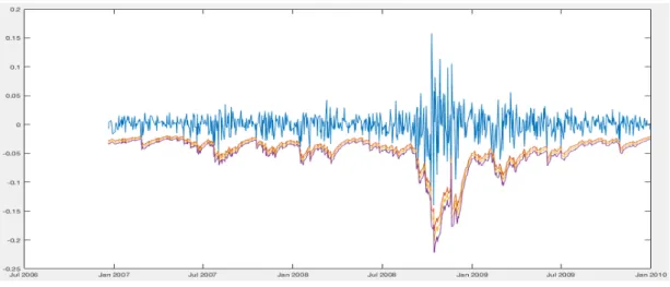
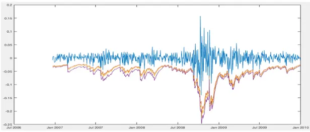
FIGURE 15: HES- TSO- VLO- COP’S ADJUSTED LOG RETURNS PLOT 97 FIGURE 16: ENERGY PORTFOLIO’S LOG RETURNS PLOT 98 FIGURE 17: 95%, 97% AND 99% VALUE-AT-RISK PLOT OF THE HISTORICAL SIMULATIONS

METHOD 99

FIGURE 18: 99,5%, 99,75% AND 99,9% VALUE-AT-RISK PLOT OF THE HISTORICAL SIMULATIONS

METHOD 99

FIGURE 19: 95%, 97% AND 99% VALUE-AT-RISK PLOT OF THE GJR(2,1) WITH GAUSSIAN

DISTRIBUTED ERRORS 103

FIGURE 20: 99,5%, 99,75% AND 99,9% VALUE-AT-RISK PLOT OF THE GJR(2,1) WITH GAUSSIAN

FIGURE 21: 95%, 97% AND 99% VALUE-AT-RISK PLOT OF THE HULL AND WHITE METHOD

ADOPTING THE GJR(2,1) WITH GAUSSIAN DISTRIBUTED ERRORS 110

FIGURE 22: 99,5%, 99,75% AND 9,99% VALUE-AT-RISK PLOT OF THE HULL AND WHITE

METHOD ADOPTING THE GJR(2,1) WITH GAUSSIAN DISTRIBUTED ERRORS 110 FIGURE 23: 95%, 97% AND 99% VALUE-AT-RISK PLOT OF THE FILTERED HISTORICAL

SIMULATION METHOD ADOPTING THE GJR(2,1) WITH GAUSSIAN DISTRIBUTED ERRORS

117

FIGURE 24: 99,5%, 99,75% AND 99,9% VALUE-AT-RISK PLOT OF THE FILTERED HISTORICAL

118

FIGURE 25: 95%, 97% AND 99% VALUE-AT-RISK PLOT OF THE CONDITIONAL VARIANCE

COVARIANCE METHOD COMBINED WITH THE HISTORICAL SIMULATION ADOPTING THE

(11)

FIGURE 26: 99,5%, 99,75% AND 99,9% VALUE-AT-RISK PLOT OF THE CONDITIONAL VARIANCE

GJR(2,1) WITH GAUSSIAN DISTRIBUTED ERRORS 126

FIGURE 27: 95%, 97% AND 99% VALUE-AT-RISK PLOT OF THE UNCONDITIONAL EXTREME

VALUE THEORY APPROACH 131

FIGURE 28: 99,5%, 99,75% AND 99,9% VALUE-AT-RISK PLOT OF THE UNCONDITIONAL

EXTREME VALUE THEORY APPROACH 131

FIGURE 29: 95%, 97% AND 99% VALUE-AT-RISK PLOT OF THE CONDITIONAL EXTREME VALUE

THEORY APPROACH ADOPTING THE GJR(2,1) 133

FIGURE 30: 99,5%, 99,75% AND 99,9% VALUE-AT-RISK PLOT OF THE CONDITIONAL EXTREME

VALUE THEORY APPROACH ADOPTING THE GJR(2,1) 134

FIGURE 31: MS- C- BAC- CS’S ADJUSTED PLOT PRICES 144

FIGURE 32: JPM- BK- GS- AXP’S ADJUSTED PLOT PRICES 145

FIGURE 33: FMCC- STD- HIG- FNM’S ADJUSTED PLOT PRICES 145

FIGURE 34: COMPANIES’ADJUSTED PRICES PLOT 146

FIGURE 35: MS- C- BAC- CS’S ADJUSTED LOG RETURNS PLOT 146

FIGURE 36: JPM- BK- GS- AXP’S ADJUSTED LOG RETURNS PLOT 147

FIGURE 37: FMCC- STD- HIG- FNM’S ADJUSTED LOG RETURNS PLOT 147

FIGURE 38: FINANCE PORTFOLIO’S LOG RETURNS PLOT 148

FIGURE 39: 95%, 97% AND 99% VALUE-AT-RISK PLOT OF THE HISTORICAL SIMULATIONS

METHOD 149

FIGURE 40: 99,5%, 99,75% AND 99,9% VALUE-AT-RISK PLOT OF THE HISTORICAL SIMULATIONS

METHOD 149

FIGURE 41: 95%, 97% AND 99% VALUE-AT-RISK PLOT OF THE GJR(1,1) WITH GAUSSIAN

FIGURE 42: 99,5%, 99,75% AND 99,9% VALUE-AT-RISK PLOT OF THE GJR(1,1) WITH GAUSSIAN

FIGURE 43: 95%, 97% AND 99% VALUE-AT-RISK PLOT OF THE HULL AND WHITE METHOD

FIGURE 44: 99,5%, 99,75% AND 9,99% VALUE-AT-RISK PLOT OF THE HULL AND WHITE

METHOD ADOPTING THE GJR(1,1) WITH GAUSSIAN DISTRIBUTED ERRORS 159 FIGURE 45: 95%, 97% AND 99% VALUE-AT-RISK PLOT OF THE FILTERED HISTORICAL

166

FIGURE 46: 99,5%, 99,75% AND 99,9% VALUE-AT-RISK PLOT OF THE FILTERED HISTORICAL

166

FIGURE 47: 95%, 97% AND 99% VALUE-AT-RISK PLOT OF THE CONDITIONAL VARIANCE

FIGURE 48: 99,5%, 99,75% AND 99,9% VALUE-AT-RISK PLOT OF THE CONDITIONAL VARIANCE

FIGURE 49: 95%, 97% AND 99% VALUE-AT-RISK PLOT OF THE UNCONDITIONAL EXTREME

VALUE THEORY APPROACH 178

FIGURE 50: 99,5%, 99,75% AND 99,9% VALUE-AT-RISK PLOT OF THE UNCONDITIONAL

EXTREME VALUE THEORY APPROACH 179

FIGURE 51: 95%, 97% AND 99% VALUE-AT-RISK PLOT OF THE CONDITIONAL EXTREME VALUE

(12)

FIGURE 52: 99,5%, 99,75% AND 99,9% VALUE-AT-RISK PLOT OF THE CONDITIONAL EXTREME

VALUE THEORY APPROACH ADOPTING THE GJR(1,1) 181

FIGURE 53: 95%, 97% AND 99% VALUE-AT-RISK PLOT OF THE ALTERNATIVE APPROACH 195

FIGURE 54: 99,5%, 99,75% AND 99,9% VALUE-AT-RISK PLOT OF THE ALTERNATIVE APPROACH

196

FIGURE 55: 95%, 97% AND 99% VALUE-AT-RISK PLOT OF THE ALTERNATIVE APPROACH 201

FIGURE 56: 99,5%, 99,75% AND 99,9% VALUE-AT-RISK PLOT OF THE ALTERNATIVE APPROACH

(13)

INDEX OF TABLES

TABLE 1: DESCRIPTIVE STATISTICS OF THE 2 PORTFOLIOS IN THE TESTING PERIOD 87

TABLE 2: N° OF VIOLATIONS AND EMPIRICAL PROBABILITIES OF A VIOLATION IN THE

HISTORICAL SIMULATIONS METHOD 100

TABLE 3: KUPIEC’S TEST OF THE HISTORICAL SIMULATIONS METHOD 100 TABLE 4: COMPUTED LAGS OF THE DIFFERENT GARCH MODELS 102

TABLE 5: N° OF VIOLATIONS AND EMPIRICAL PROBABILITIES OF A VIOLATION OF THE

CONDITIONAL VARIANCE COVARIANCE METHOD 104

TABLE 6: KUPIEC’S TEST OF THE CONDITIONAL VARIANCE COVARIANCE METHOD 105 TABLE 7: CHRISTOFFERSEN’S TEST OF THE GARCH(2,1) WITH GAUSSIAN DISTRIBUTED ERRORS

106

TABLE 8: CHRISTOFFERSEN’S TEST OF THE EGARCH(1,1) WITH GAUSSIAN DISTRIBUTED

ERRORS 106

TABLE 9: CHRISTOFFERSEN’S TEST OF THE GJR(2,1) WITH GAUSSIAN DISTRIBUTED ERRORS106

TABLE 10: CHRISTOFFERSEN’S TEST OF THE GARCH(1,1) WITH T DISTRIBUTED ERRORS 107

TABLE 11: CHRISTOFFERSEN’S TEST OF THE EGARCH(1,1) WITH T DISTRIBUTED ERRORS 107

TABLE 12: CHRISTOFFERSEN’S TEST OF THE GJR(1,1) WITH T DISTRIBUTED ERRORS 107

TABLE 13: QUADRATIC LOSS VALUE OF THE CONDITIONAL VARIANCE COVARIANCE METHOD

109

TABLE 14: N° OF VIOLATIONS AND EMPIRICAL PROBABILITIES OF A VIOLATION OF THE HULL

AND WHITE METHOD 111

TABLE 15: KUPIEC’S TEST OF THE HULL AND WHITE METHOD 112

TABLE 16: CHRISTOFFERSEN’S TEST OF THE HULL AND WHITE METHOD ADOPTING THE

GARCH(2,1) WITH GAUSSIAN DISTRIBUTED ERRORS 113

EGARCH(1,1) WITH GAUSSIAN DISTRIBUTED ERRORS 113

GARCH(1,1) WITH T DISTRIBUTED ERRORS 114

EGARCH(1,1) WITH T DISTRIBUTED ERRORS 114

GJR(1,1) WITH T DISTRIBUTED ERRORS 115

TABLE 22: QUADRATIC LOSS VALUE OF THE HULL AND WHITE METHOD 116 TABLE 23: N° OF VIOLATIONS AND EMPIRICAL PROBABILITIES OF A VIOLATION OF THE

FILTERED HISTORICAL SIMULATION METHOD 119

(14)

TABLE 25: CHRISTOFFERSEN’S TEST OF THE FILTERED HISTORICAL SIMULATION METHOD

ADOPTING THE GARCH(2,1) WITH GAUSSIAN DISTRIBUTED ERRORS 121

ADOPTING THE EGARCH(1,1) WITH GAUSSIAN DISTRIBUTED ERRORS 121 TABLE 27: CHRISTOFFERSEN’S TEST OF THE FILTERED HISTORICAL SIMULATION METHOD

ADOPTING THE GARCH(1,1) WITH T DISTRIBUTED ERRORS 122 TABLE 29: CHRISTOFFERSEN’S TEST OF THE FILTERED HISTORICAL SIMULATION METHOD

ADOPTING THE EGARCH(1,1) WITH T DISTRIBUTED ERRORS 122

ADOPTING THE GJR(1,1) WITH T DISTRIBUTED ERRORS 123

TABLE 31: QUADRATIC LOSS VALUE OF THE FILTERED HISTORICAL SIMULATIONS METHOD 124

VARIANCE COVARIANCE METHOD COMBINED WITH HISTORICAL SIMULATIONS 126

TABLE 33: KUPIEC’S TEST OF THE CONDITIONAL VARIANCE COVARIANCE METHOD COMBINED

WITH HISTORICAL SIMULATIONS 127

TABLE 34: CHRISTOFFERSEN’S TEST OF THE VARIANCE COVARIANCE METHOD COMBINED

WITH THE HISTORICAL SIMULATIONS ADOPTING THE GARCH(2,1) 128

WITH THE HISTORICAL SIMULATIONS ADOPTING THE EGARCH(1,1) 128

WITH THE HISTORICAL SIMULATIONS ADOPTING THE GJR(2,1) 128 TABLE 37: QUADRATIC LOSS VALUE OF THE CONDITIONAL VARIANCE COVARIANCE METHOD

COMBINED WITH THE HISTORICAL SIMULATIONS 129

UNCONDITIONAL EXTREME VALUE THEORY APPROACH 132

TABLE 39: KUPIEC’S TEST OF THE UNCONDITIONAL EXTREME VALUE THEORY APPROACH 132

CONDITIONAL EXTREME VALUE THEORY APPROACH 134

TABLE 41: KUPIEC’S TEST OF THE CONDITIONAL EXTREME VALUE THOERY APPROACH 135 TABLE 42: CHRISTOFFERSEN’S TEST OF THE CONDITIONAL EXTREME VALUE THEORY

APPROACH ADOPTING THE GARCH(2,1) 136

TABLE 43: CHRISTOFFERSEN’S TEST OF THE CONDITIONAL EXTREME VALUE THEORY

APPROACH ADOPTING THE EGARCH(1,1) 136

APPROACH ADOPTING THE GJR(2,1) 136

TABLE 45: QUADRATIC LOSS VALUE OF THE CONDITIONAL EXTREME VALUE THEORY

APPROACH 137

TABLE 46: BEST PERFORMING VARIANTS FOR EACH APPROACH 139

TABLE 47: QUADRATIC LOSS AND SQUARE ROOT OF THE MEAN QUADRATIC LOSS OF THE BEST

PERFORMING MODELS 140

HISTORICAL SIMULATIONS METHOD 150

TABLE 49: KUPIEC’S TEST OF THE HISTORICAL SIMULATIONS METHOD 150 TABLE 50: COMPUTED LAGS OF THE DIFFERENT GARCH MODELS 151

CONDITIONAL VARIANCE COVARIANCE METHOD 153

(15)

TABLE 53: CHRISTOFFERSEN’S TEST OF THE GARCH(1,1) WITH GAUSSIAN DISTRIBUTED

ERRORS 155

TABLE 54: CHRISTOFFERSEN’S TEST OF THE EGARCH(2,1) WITH GAUSSIAN DISTRIBUTED

ERRORS 155

TABLE 55: CHRISTOFFERSEN’S TEST OF THE GJR(1,1) WITH GAUSSIAN DISTRIBUTED ERRORS

155

TABLE 56: CHRISTOFFERSEN’S TEST OF THE GARCH(1,1) WITH T DISTRIBUTED ERRORS 156

TABLE 57: CHRISTOFFERSEN’S TEST OF THE EGARCH(1,1) WITH T DISTRIBUTED ERRORS 156 TABLE 58: CHRISTOFFERSEN’S TEST OF THE GJR(1,1) WITH T DISTRIBUTED ERRORS 156 TABLE 59: QUADRATIC LOSS VALUE OF THE CONDITIONAL VARIANCE COVARIANCE METHOD

158

TABLE 60: N° OF VIOLATIONS AND EMPIRICAL PROBABILITIES OF A VIOLATION OF THE HULL

AND WHITE METHOD 160

TABLE 61: KUPIEC’S TEST OF THE HULL AND WHITE METHOD 161

GARCH(1,1) WITH GAUSSIAN DISTRIBUTED ERRORS 162

EGARCH(2,1) WITH GAUSSIAN DISTRIBUTED ERRORS 162

GARCH(1,1) WITH T DISTRIBUTED ERRORS 163

EGARCH(1,1) WITH T DISTRIBUTED ERRORS 163

GJR(1,1) WITH T DISTRIBUTED ERRORS 164

TABLE 68: QUADRATIC LOSS VALUE OF THE HULL AND WHITE METHOD 165 TABLE 69: N° OF VIOLATIONS AND EMPIRICAL PROBABILITIES OF A VIOLATION OF THE

FILTERED HISTORICAL SIMULATION METHOD 167

TABLE 70: KUPIEC’S TEST OF THE FILTERED HISTORICAL SIMULATIONS METHOD 168

ADOPTING THE GARCH(1,1) WITH GAUSSIAN DISTRIBUTED ERRORS 169

ADOPTING THE EGARCH(2,1) WITH GAUSSIAN DISTRIBUTED ERRORS 169

ADOPTING THE GARCH(1,1) WITH T DISTRIBUTED ERRORS 170

ADOPTING THE EGARCH(1,1) WITH T DISTRIBUTED ERRORS 170

ADOPTING THE GJR(1,1) WITH T DISTRIBUTED ERRORS 170

TABLE 77: QUADRATIC LOSS VALUE OF THE FILTERED HISTORICAL SIMULATIONS METHOD 172

CONDITIONAL VARIANCE COVARIANCE METHOD COMBINED WITH HISTORIACAL

SIMULATIONS 174

TABLE 79: KUPIEC’S TEST OF THE CONDITIONAL VARIANCE COVARIANCE METHOD COMBINED

(16)

WITH THE HISTORICAL SIMULATIONS ADOPTING THE GARCH(1,1) 176

WITH THE HISTORICAL SIMULATIONS ADOPTING THE EGARCH(2,1) 176 TABLE 82: CHRISTOFFERSEN’S TEST OF THE VARIANCE COVARIANCE METHOD COMBINED

WITH THE HISTORICAL SIMULATIONS ADOPTING THE GJR(1,1) 176

TABLE 83: QUADRATIC LOSS VALUE OF THE CONDITIONAL VARIANCE COVARIANCE METHOD

COMBINED WITH THE HISTORICAL SIMULATIONS 177

UNCONDITIONAL EXTREME VALUE THEORY APPROACH 179

TABLE 85: KUPIEC’S TEST OF THE UNCONDITIONAL EXTREME VALUE THOERY APPROACH 180

CONDITIONAL EXTREME VALUE THEORY APPROACH 181

TABLE 87: KUPIEC’S TEST OF THE CONDITIONAL EXTREME VALUE THOERY APPROACH 182

APPROACH ADOPTING THE GARCH(1,1) 183

APPROACH ADOPTING THE EGARCH(2,1) 183

APPROACH ADOPTING THE GJR(1,1) 183

TABLE 91: QUADRATIC LOSS VALUE OF THE CONDITIONAL EXTREME VALUE THEORY

APPROACH 184

TABLE 92: BEST PERFORMING VARIANTS FOR EACH APPROACH 185 TABLE 93: QUADRATIC LOSS AND SQUARE ROOT OF THE MEAN QUADRATIC LOSS OF THE BEST

PERFORMING MODELS 186

TABLE 94: N° OF VIOLATIONS AND EMPIRICAL PROBABILITIES OF A VIOLATION IN THE

ALTERNATIVE APPROACH 196

TABLE 95: KUPIEC’S TEST OF THE ALTERNATIVE APPROACH 197

TABLE 96: CHRISTOFFERSEN’S TEST OF THE ALTERNATIVE 197

TABLE 97: QUADRATIC LOSS VALUE OF THE ALTERNATIVE APPROACH 197

ALTERNATIVE APPROACH 202

TABLE 99: KUPIEC’S TEST OF THE ALTERNATIVE APPROACH 202

TABLE 100: CHRISTOFFERSEN’S TEST OF THE ALTERNATIVE 203

(17)

(18)

1. INTRODUCTION TO FINANCIAL RISK

MANAGEMENT

Financial Risk Management is the practice adopted by organizations in order to identify and measure the main financial risks to which they are exposed, with the purpose to manage their impact. Managing such risks is an important step of any organisation’s strategic and operational activities. The role of risk management is to monitor risks and undertaking actions to minimise their impact. This statement can be extended to financial risk management, defining it as the task of monitoring financial risks and managing their impact. It is a sub-discipline of the wider function of risk management and it makes an extensive use of financial theory. Financial risk management is included in the financial function of an organisation. Traditionally, the financial function has been seen in terms of financial reporting and control. The modern approach is to consider the financial function in terms of financial policy and financial decision-making.

1.1. HISTORY

Financial risk management as a concept has been always present in people life. Information about forward deals can be found in India in 2000 b.C., as well as in the ancient Rome concerning the grain market. Even merchant during the Middle age attempted to reduce their risks by pooling capital through collective ventures, reaching a certain level of diversification. In 1571 in London was built the Royal Exchange giving rise to a forward market in which people were used to buy and sell contracts in order to reduce the price risk as well as the delivery one.

During IXX century risk management made a step forward with the creation of organised terminal for the exchange of risks on the agriculture commodities, first in New York and Chicago and then even in other European cities.

(19)

Financial risk management started to increase its importance becoming a responsibility of managers after two important events:

1. The big increase in volatility in the foreign exchange markets, due to the decision of the USA to stop trading dollars for gold at a fixed price of 35$ per oz. This increase in volatility had an effect on many other markets such as the commodities one. This troubles in the foreign exchange markets allowed local countries to pursue different economic policies, whose effect were propagated through the exchange rate, leading to an increase of the economic complexity;

2. The first oil shocks of 1973, which caused a quadruplication of the oil price. Other oil shocks have been pushed by government, causing an increase in extreme value in the oil price series. This was obviously a problem for oil producer as well as consumers, leading to an increase of the demand of risk management instruments.

After these two important events, other episodes contributed to the increase in market volatility. The most important one was the recent financial crisis that brought to its knees the global economy, forcing the regulator to ask for more stringent risk management policies.

(20)

1.2. MAIN TYPOLOGIES OF FINANCIAL

RISK

Financial risk is the general term to indicate a larger number of different types of risk that are related to financial activities.

The main typologies of financial risk may be included into four macro areas:

1. Market risk: it is the risk to incur in a loss due to changes in the value of a financial position held by the company. If it holds a large investment in stocks, it is exposed to the risk that those stocks will drop in value generating a loss. Investors who operates in financial markets must deal with it;

2. Credit risk: it is the risk to incur in a loss generated by the inability of the counterparty to repay a part or the total amount of the borrowed funds. Generally, banks that lend money to individuals/companies must manage it. There is a wide literature on credit risk and in particular on the estimation of correlation among borrowers;

3. Liquidity risk: it is the risk to incur in a loss generated by the lack of marketability of an investment that cannot be bought or sold quickly when needed. Liquidity is an important characteristic of financial markets. The more an investment is liquid, the better it is;

4. Operational risk: it is the risk to incur in a loss resulting from inadequate or failed internal processes, people and systems or from external events. This definition includes legal risk, but excludes strategic and reputational risk. An example of operational risk is the lack of control over traders’ actions.

This list above is far from representing an accurate and complete categorisation of risk, but it includes the most important and studied ones.

(21)

1.3. WHY MANAGING FINANCIAL RISK?

One of the principal functions of risk management in the financial sector is to determine the amount of capital that a financial institution is required to hold, to be protected against unexpected future losses on its portfolio, in order to satisfy a regulator who is concerned with the solvency of the institution. The purpose of bank regulation is to assure that a bank keeps enough capital in relation to the risk that it decides to take, as banks have a systemic impact on the economy.

Systemic risk is defined as the risk that a default of a financial institution will create a “ripple effect” leading to the default of other financial institutions, damaging the stability of the entire economic system. Regulator is concerned about avoiding such a situation as it would create panic, pushing people to rapidly withdraw their money (bank run)

1.3.1. Regulatory capital

In 1988, through an agreement called Basel Accord, banks started to be regulated by international risk-based standards for capital adequacy. Before that date, the regulation of banks was done setting minimum levels of the capital’s ratio to total assets. These levels varied country-by-country depending on different factors.

The agreement signed in 1988, called Basel I, established minimum capital requirements that bank must hold. This accord was mainly focused on Credit risk by associating an appropriate risk-weight to the assets of a bank: the riskier is the type of asset, the higher will be the risk-weight. For example, it is given 0% weight to Treasuries while 50% to residential mortgage.Therefore, an international bank was required to hold an amount of capital equal to the 8% of their risk-weighted assets (RWA). The capital is composed by:

• Tier 1 Capital: this category includes equity and noncumulative perpetual preferred stock;

(22)

• Tier 2 Capital: refers to the supplementary capital that includes cumulative perpetual preferred stock, subordinated debt with an original life of more than five years and other kind of hybrid instruments.

Equity capital is the most important one since it absorbs losses when they occur. Indeed, the 50% of the capital must be Tier 1.

In 1996 the Basel Committee issued the so called 1996 Amendment, which introduced a new source of risk: market risk for trading activity, which in turn led to an increased amount of capital requirement.

In 2004 a new set of laws made the entrance in banking regulation with the name of

Basel II, replacing the old Basel I; it took some years before it was implemented by

banks.

The aim of Basel II was to ensure that the greater is the risk to which a bank is exposed, the larger is the amount of capital it has to hold to cover it.

This new regulation was based on three pillars:

1. Minimum capital requirement: the regulatory capital must be calculated for Credit risk (three different approaches are allowed to compute it), Market Risk (Value-at-Risk is employed) and Operational Risk (again three approaches are allowed for the computation).

The total capital is then calculated using this formula:

𝐶𝑎𝑝𝑖𝑡𝑎𝑙 = 8%( 𝐶𝑟𝑒𝑑𝑖𝑡𝑅𝑖𝑠𝑘 𝑅𝑊𝐴 + 𝑀𝑎𝑟𝑘𝑒𝑡𝑅𝑖𝑠𝑘 𝑅𝑊𝐴 + 𝑂𝑝𝑒𝑟𝑎𝑡𝑖𝑜𝑛𝑎𝑙𝑅𝑖𝑠𝑘 𝑅𝑊𝐴)

2. Supervisory review: the regulator must assure that a bank uses adequate and reliable processes, both quantitative and qualitative, to ensure that minimum level of capital are maintained;

(23)

information to the market about the risks they take and the way in which these risks are managed.

As this dissertation focuses on Market risk, some precisions have to be done. In

Basel II framework the capital requirement for Market risk is calculated in this way:

𝑀𝑘𝑡𝑅𝑖𝑠𝑘𝐶𝑎𝑝𝑖𝑡𝑎𝑙: = max 𝑉𝑎𝑅: 0.01 , 𝑚D 1 60 𝑉𝑎𝑅:FG(0.01 HI JKL ) + 𝐶 Where 𝑉𝑎𝑅_: and _MLG HI 𝑉𝑎𝑅_:FG

JKL are respectively the Value-at-Risk estimated for

time t and the average one over the last 60 days. The confidence level 𝛼 is equal to 99% while 𝑚D is a multiplication factor applied to the average VaR.

Clearly, the higher the VaR is, the higher will be the capital to be set aside. Moreover, the capital requirement depends also on the accuracy of the VaR estimation, through 𝑚_D.

It can be easily understood looking at the analytical definition of 𝑆_: :

𝑚_D =

3.0 𝑖𝑓 𝑁 ≤ 4 3 + 0.2 𝑁 − 4 𝑖𝑓 5 ≤ 𝑁 ≤ 9 4.0 𝑖𝑓 10 < 𝑁

Where N is the number of VaR violations in the previous 250 days. This part will be clearer later, when the definition of Value-at-Risk will be given as well as the meaning of backtesting explained. It is important to point out that the lower the accuracy of a VaR measure is, the higher is the capital that a bank is required to hold.

During the financial crisis, it came out that the calculation of the regulatory capital for market risk needed some changes. These changes were contained in Basel II.5. In particular, it was introduced the calculation of a stressed VaR, which is the Value-at-Risk calculated in a period characterized by big movements in market variables. Therefore, the formula used to calculate market risk capital requirement changed. It is the following:

(24)

𝑀𝑘𝑡𝑅𝑖𝑠𝑘𝐶𝑎𝑝𝑖𝑡𝑎𝑙_: = max 𝑉𝑎𝑅_: 0.01 , 𝑚_D 1 60 𝑉𝑎𝑅:FG(0.01 HI JKL ) + max 𝑠𝑉𝑎𝑅_: 0.01 , 𝑚_Z 1 60 𝑠𝑉𝑎𝑅:FG(0.01 HI JKL )

A typical period used to compute the stressed VaR is the financial crisis, but every bank is free to use a different one as long as it has to be coherent with its portfolio.

Finally, after the financial crisis and the collapse of Lehman Brothers, the Basel Committee decided to increment the restrictions over banks developing Basel III. It introduces two buffers of capital, the Countercyclical and the Capital Conservation, leading to an increase in the thresholds of Tier I; two ratios to be satisfied, the Leverage ratio and the Net Stable Funding ratio (which refers to Liquidity risk); the Counterparty Credit risk. The implementation of Basel III is still on going (from 2013 until 2019).

1.4. BASICAL MATHEMATICAL CONCEPT

One of the most important issues in Financial Risk Management is the measurement of such risks. The discipline that aims at addressing this problem is called Quantitative Risk Management and it is continuously improving. It makes use of mathematics, probability and statistics theory.

Below I am going to present some mathematical tools which are very important in this field.

(25)

1.4.1. Risk factors, loss operator and loss

distributions

A probability space, indicated with the following terminology Ω, ℱ, Ρ , is used to describe the domain of the random variables used in this framework to indicate the future state of the world.

Consider a portfolio containing financial assets such as stocks, bonds, derivatives or other kind of instruments; denote the value of this portfolio at time t with 𝑉 𝑡 . The loss at time t+1 is given by:

𝐿:_G= − 𝑉 𝑡 + 1 − 𝑉 𝑡

The minus before the expression means that the loss is expressed as a positive value. Obviously, we can observe 𝐿_{:_G} only at time

t+1, while it is unknown at time

t.

The distribution of 𝐿_{:_G} is called “loss distribution” and it is one of the most important concepts in all the typologies of risk. Practitioners in risk management are used to model the value of the portfolio as a function of the time and the risk factors.

𝑉_: = 𝑓 𝑡 , 𝑍_:

This representation is known with the name of mapping.

Risk factors are observable objects on which the value of the portfolio depends. Different risk factors could be chosen depending on the level of precision that we want to achieve and depending on the composition of the portfolio. For example in a stock portfolio we would use logarithmic prices, in a bond portfolio we will use the yield of such bonds.

It is assumed that risk factors are known at time

t. Actually, what is used in the

analysis is not the series of the risk factors but the series of the risk factors changes, indicated with 𝑋_:. Changes in the risk factors cause changes in the value of the

(26)

Therefore, the value of the portfolio loss at time t+1 can be written as follows:

𝐿_{:_G}= − 𝑓 𝑡 + 1, 𝑍_:+ 𝑋_{:_G} − 𝑓 𝑡 , 𝑍_:

In this expression we can see that the value of the loss at time t+1 depends only on the value of the risk factor at time t+1 and so we can express 𝐿:_G as a function of

𝑋_{:_G} obtaining the following notation:

𝐿_{:_G} = 𝑙_[:] 𝑋_{:_G} (1)

where 𝑙_[:] is called Loss Operator. It maps risk factor changes into losses:

𝑙_[:]= − 𝑓 𝑡 + 1, 𝑍_:+ 𝑥 − 𝑓 𝑡 , 𝑍_:

It is possible to obtain a linearized version of the loss operator if 𝑓 is differentiable with respect to 𝑡 and 𝑍_:, by using a first order Taylor expansion of 𝐿_{:_G}

𝐿∆_{:_G}_{= − 𝑓}

: 𝑡 , 𝑍: − 𝑓fg

h

JKG

𝑡 , 𝑍_: 𝑋_{:_G,J}

Where 𝑓_: denotes the partial derivative of 𝑓 with respect to t and 𝑓_f_g the partial derivative of 𝑓 with respect to the i risk factor. The linearized loss operator is then:

𝑙_[:]∆ _{𝑥 = − 𝑓}

: 𝑡 , 𝑍: − 𝑓fg

h

JKG

𝑡 , 𝑍_: 𝑥_J

Using the linear approximation, we can express the loss distribution as a linear function of the risk factor changes. The price to pay is the error generated by this approximation, which is higher as the time horizon increases.

(27)

A short time horizon is also more coherent with the hypothesis of no changes in the portfolio (no rebalancing and no changing in composition).

Finally, it is important to clarify the difference between conditional and

unconditional loss distribution. In the first one, we are interested in the distribution

of 𝐿:_G given all the information up to time t. This set of information, also called

“history”, is indicated by ℱ_:. It is used mainly with short time horizon and it is extremely important. It is defined as the distribution of the loss operator under the conditional distribution of the risk factor changes and it is written as follow:

𝐹jklm|ℱk 𝑙 = 𝑃 𝑙[:] 𝑋:_G ≤ 𝑙 | ℱ: = 𝑃 𝐿:_G ≤ 𝑙 | ℱ:

The unconditional loss distribution instead is indicated with 𝐹_j_klm and it is the distribution of the loss operator when the risk factor changes have a stationary distribution, which means that their distribution is time invariant. It tends to be used in application with a longer time horizon such as in credit risk analysis.

When risk factor changes form an iid sequence, conditional and unconditional loss distribution are the same object.

1.5. COHERENT RISK MEASURES

With the term coherent risk measure we indicate a list of properties that a risk measure should have in order to be considered good and reliable. A list of properties was proposed in a paper by Artzner et al. (1999).

Therefore, a coherent risk measure is a real-valued function 𝜚 on same space of random variables, representing losses, which satisfies the following four properties:

1. Monotonicity: for 2 random variables with 𝐿_G ≥ 𝐿_r we will have

(28)

It is quite simple to understand, as the more is the loss generated, the higher should be the risk detected by the measure as well as the capital to keep aside;

2. Positive homogeneity: for 𝜆 ≥ 0 we have that 𝜚 𝜆𝐿 =

𝜆𝜚 𝐿 .

It means that if you scale the loss of a value 𝜆 , the risk measure should be scaled of the same 𝜆;

3. Translation Invariance: for any 𝑎 ∈ ℝ we have that 𝜚 𝐿 +

𝑎 = 𝜚 𝐿 + 𝑎 .

It means that if our loss increases of a level 𝑎 , the risk measure should increase of 𝑎. On the other hand, if an amount of cash 𝑎 is added to the portfolio, the risk measure should decrease of the amount 𝑎;

4. Subadditivity: for any 𝐿G , 𝐿r we have that 𝜚 𝐿G+ 𝐿r ≤

𝜚 𝐿_G + 𝜚 𝐿_r .

It means that if we mix two portfolios, the risk measure should be lower than the sum of the one of the two separate portfolios. This is one of the most problematic properties because if a regulator uses a non-sub additive risk measure, financial institutions are incentivised to split themselves into subsidiaries in order to minimize risk regulatory capital. Other problems of non-subadditivity are related to the concept of diversification and the decentralization of risk management systems.

(29)

2. VALUE-AT-RISK AS A MEASURE OF

MARKET RISK

Value-at-risk is an important measure of risk and, as we have seen in the section above, since Basel II was implemented, it has been used by regulators to determine the regulatory capital that a bank must keep aside for the risk it takes. Value-at-risk is not only used in market risk, but even in Credit risk to determine for example the Credit VaR of a securitized portfolio, in Operational risk in the AMA approach ecc. It is a very important risk measure and it is very simple to understand, synthetizing in a single number a large amount of information.

2.1. BIRTH AND HISTORY

The concept of Value-at-Risk enters officially in finance industry in 1990, but the attempts to measure the risk of a portfolio started much earlier. The first who tried to do this was Francis Edgeworth in 1988, who used past data to estimate future probabilities.

Markowitz(1952) did other trials, employing the variance covariance matrix of the assets included in the portfolio. His method had a strong limitation since it requires the subjective opinion of experts in addition to statistical techniques. Few months later, Arthur D. Roy(1952) proposed another similar risk measure, which made use of the variance covariance matrix of the risk factors as well as the vector of average losses. The job to find a reliable risk measure became more difficult with the increasing of the number of different financial products, due to the increasing in complexity and to the absence of historical data related to them. Moreover, during the 70th years many countries started to develop their own currency and this make increase the intricacy of the problem.

(30)

Finally, just at the beginning of the 90th years, Value-at-Risk in its modern interpretation made its entry in the industry. The merit of this event was given mainly to JP Morgan, one of the bigger investment banks in the world. Precisely, the chairman of the bank, Dennis Weatherstone, was fed up with the size of the risk report that arrived continuously in his office and asked to its employees to provide to him a risk measure which is much more simple to understand and that could give a more comprehensive picture of the bank’s exposure in a single number. The introduction of this new measure was a very revolution and other banks started to use it. In addition, many software companies decided to exploit the situation by developing programmes, whose aim was to compute the VaR. In the 1994, JP Morgan published a simplified version of this approach, calling it Risk metrics.

2.2. MATHEMATICAL DEFINITION

Let’s now discuss the mathematical details of the Value-at-Risk. As already mentioned, it is a number that indicates a loss that will not be exceed with a specific probability (1 - confidence level) in a specific time horizon.

Mathematically it could be defined in this way:

Given some confidence level 𝛼 ∈ 0,1 , Value-at-Risk of a portfolio at that confidence level is given by the smallest number 𝑙, such that the loss 𝐿 in which you will incur in the time horizon T will exceed 𝑙 with a probability not larger than (1 − 𝛼).

In mathematical terms it is written as:

𝑽𝒂𝑹_∝= inf 𝑙 ∈ 𝑅: 𝑃 𝐿 > 𝑙 ≤ 1 − 𝛼 = inf {𝑙 ∈ 𝑅: 𝐹_j(𝑙) ≥ 𝛼}

To make things more clear, let’s suppose you have calculated that your Value-at-Risk for the next year with a confidence level of 95%, is 1 billion Euros. Then the probability that you will incur in a loss higher than 1 billion in the next year, is lower than 5%.

(31)

Basically, in the probabilistic language, it is defined as the 𝛼-percentile of the loss distribution. Indeed, as is shown in the formula, a probability distribution 𝐹_j is assumed, clearly the loss distribution is unknown.

Figure 1: EXAMPLE OF LOSS DISTRIBUTION

In figure 1 we can observe an example of loss distribution: in the horizontal axis are reported the losses in absolute value while in the vertical axis the probability associated to that losses. As can be seen from the figure, loss distributions are characterised by longer right tails.

In the figure are signed both the expected loss, the VaR and the expected Shortfall, that we will present later. As we can see the 𝑉𝑎𝑅_•, with 𝛼 = 0,95 , is the loss that will not be exceeded with a probability of 95% along a pre-specified time horizon T.

When speaking about Value-at-Risk, it is important to illustrate the concept of quantile function, which is strictly related to it.

The quantile function of a density function F is its generalized inverse and it is indicated as 𝐹←_{. Let F : ℝ → 0,1 be an arbitrary CDF, then for 𝛼 ∈ 0,1 the}

𝛼-quantile of F is defined by:

𝑞• 𝐹 ∶= 𝑖𝑛𝑓 𝑥 ∈ ℝ ∶ 𝐹 𝑥 ≥ 𝛼

(32)

In case F is not continuously or strictly increasing, the convention imposes to take the first point, call it 𝑙_G (in case of a loss distribution it is the first loss) such that the following conditions hold:

- 𝐹(𝑙) ≥ 𝛼 for all the 𝑙 ≥ 𝑙_G - 𝐹(𝑙) < 𝛼 for all the 𝑙 < 𝑙_G

Thus the VaR at the confidence interval 𝛼 ∈ 0,1 is then:

𝑉𝑎𝑅_•: = 𝑞_• 𝐹_j (2)

Typical values for 𝛼 are 0.95 and 0.99, while the time horizon depends on the typology of risk we are interested in measure: in market risk management T goes from 1 to 10 days, while in credit and operational risk management T is usually 1 year.

2.3. SHORTCOMING OF VaR and

EXPECTED SHORTFALL

After what we have just said, it is easy to understand that VaR is only a threshold value with specific probability that will not be exceeded in a specified time horizon. Therefore, it does not say anything about what happens beyond that threshold. In other words, when the event with probability 1 − 𝛼 happens, we do not know which is the magnitude of that loss.

To clarify the concept an example has to be given: let’s suppose that we hold a stock portfolio with a market value of 1 billion € and we are interested in the VaR of the next day of that portfolio with 𝛼 = 0.99 . The value of the 𝑉𝑎𝑅_L.II has been estimated equal to 100 million €. The meaning of this measure is that there is only 1% probability that tomorrow we will incur in a loss higher than 100 million €. But, what will happen in case that event with 1% probability will verify tomorrow? The answer is that we could lose 101 million € as well as 1 billion € (the entire value of the portfolio).

(33)

The VaR measure that we have estimated does not give any information about that case. On the contrary, the regulator is very interested in this issue because he has to require to the banks to hold enough capital to cover that specific loss event.

To overcome this problem another risk measure has been developed with the name of “Expected Shortfall”. It is defined as the average loss of a portfolio given that a loss higher than the VaR is occurred. This is why in literature is called Conditional VaR.

In mathematical terms we can express ES in this way:

𝐸S_• = 1

1 − 𝛼 𝑞ˆ

G •

𝐹_j 𝑑𝑢

where 𝐹_j is the density function of the loss distribution and 𝑞_ˆ 𝐹_j is its u-quantile. It is clear that 𝑞_ˆ 𝐹_j = 𝑉𝑎𝑅_ˆ such that we can rewrite the expression as:

𝐸𝑆_• = 1 1 − 𝛼 𝑞ˆ G • 𝐹_j 𝑑𝑢

This expression is self-explained: the expected shortfall is the average of all the quantiles of the loss distribution that goes beyond the specified level 𝛼. Therefore, it is going into the tails in order to see what happens when the VaR is exceeded.

Another drawback of VaR is that it can’t be considered a coherent risk measure, since it does not respect the subadditivity property. In particular, it can be shown that:

𝑉𝑎𝑅• 𝐿G+ 𝐿r ≤ 𝑉𝑎𝑅• 𝐿G + 𝑉𝑎𝑅• 𝐿r

is not always true.

Again the Expected Shortfall does not have this shortcoming so it is a coherent risk measure. Regulator indeed is planning to move from a VaR based regulatory capital to an ES based one. An interesting paper analysing ES properties is Acerbi et al.(2002).

(34)

An interested reader could also give an eye to Yasuhiro et al.(2004) where the authors analytically illustrate how in some cases the tail risk of VaR could give some problems.

(35)

3. CLASSICAL VALUE AT RISK METHODS

Even if Value-at-Risk is a simple measure that indicates the risk of a portfolio in a straightforward way, it is not so simple to be estimated. Many different models have been developed from the date of its first apparition.

In the following part, I will present the first methods implemented in order to estimate the Value-at-Risk. These methods are the simplest ones and rely on very big distributional assumptions.

To homogenize the framework with the previous section, we want to estimate the quantile of the loss distribution at time t+1, which can be written as a function of the risk factor changes from time t to time t+1, as in the equation [1].

3.1. VARIANCE COVARIANCE METHOD

The variance covariance method is one of the first methods adopted for the Value-at-Risk estimation. It is a parametric method, meaning that a specific distribution is assumed for the risk factor changes.

This model, at least in its first application in the JPMorgan Riskmetrics, assumes that the vector of risk-factors changes is distributed as a multivariate normal distribution. This model relies on strong distributional assumptions and it is not used anymore in the industry.

3.1.1. Mathematical definition and application

As already mentioned above, this method assumes that the vector of risk-factors changes 𝑋_{:_G} is distributed as a multivariate normal distribution with mean 𝑢 and standard deviation represented by the variance covariance matrix Σ

(36)

Historical data of risk factors changes are used in order to estimate the mean, the variances and the co-variances.

It means that if we conduct the analysis considering the unconditional distribution of the risk factors, we can simply estimate the sample mean 𝑢 and sample variance 𝜎r

from historical data of risk factor changes [𝑋_{:F•_G}, … , 𝑋_:] and estimate the 𝑉𝑎𝑅_•,: using the following formula:

VaR_𝜶,𝒕 = 𝑢_:+ σ _:𝜙FG_(𝛼) ₍₃₎

Where 𝜙FG_{(𝛼) is the inverse of the standard normal distribution evaluated in 𝛼,}

which means that it is its 𝛼 -quantile. Note that the formula is considering the univariate case.

This model makes use of the linearized loss operator, exploiting one of the properties of the multivariate normal distribution: a linear function of a variable that is normally distributed is still normally distributed.

In our case this property says that if risk factor changes are assumed to be normal, then using a linear combination of them, it will result in a loss distribution, which is normal too.

For sake of simplicity it is assumed a loss operator of this form:

𝑙∆_: _{𝑥 = − (𝑐}

:+ 𝑤—:𝑥)

Where 𝑐_: and 𝑤—

: are constants known at time t. For example, in a stock portfolio we

have 𝑙∆_: _{𝑥 = −𝑉}

:𝑤—:𝑥, where 𝑤— is a vector of weight and 𝑉: is the value of the

portfolio at time t.

So if we assume that the linearized operator is a good approximation of the true loss we can write:

𝐿∆_{:_G}_{= 𝑙} : ∆ _𝑋

(37)

And the 𝑉𝑎𝑅_• can be easily calculated using the formula [3]

𝑉𝑎𝑅_• = −𝑐 − 𝑤—

:𝜇 + 𝑤—Σ𝑤 𝜙FG(𝛼)

Note that here the formula is extended to the multivariate case.

On the other hand, if we want to base our analysis on the conditional distribution we treat the data as a realization of a multivariate time series:

𝑋_{:_G}| ℱ_:~ 𝑁_h( 𝜇_{:_G}, Σ_{:_G})

Where 𝜇_{:_G} and Σ_{:_G} are respectively the vector of conditional means and the conditional variance covariance matrix given information up to time t ( ℱ_:). In order to get these two elements, we need to use a suitable model of forecasting such as an ARMA for the conditional mean and a GARCH for the conditional variance. We will discuss it later on.

The VaR can be estimated again using the formula [3] used in the unconditional case.

The normal distribution is not the only one allowed in this method, since it is not the only one for which linear operations can be done. Other distributions that have this property and that can be used in the variance-covariance method are the ones in the class of the generalized hyperbolic distributions among which the student t.

If we want to use the t-distribution, known for having fatter tails than the normal and so more suitable to describe financial variables, we can exploit again the above mentioned property, getting a result similar to the previous:

𝐿∆_{:_G}_{= 𝑙}

:_G∆ 𝑋:_G ~ 𝑡(𝑣 , 𝑐:− 𝑤—: , 𝑤—:Σ 𝑤:)

(38)

Value at risk can be estimated using the formula [3] as before, correcting the standard deviation forecast with ›Fr_› and using the inverse function of the

t

distribution instead of the one of the normal.

The advantage of this method is that it is simple to implement.

Despite this, it is not so used in practice because of two important weaknesses:

1) The linearization is not a good approximation of the relationship between the risk factors and the loss distribution. Indeed, this approximation employs the first order Taylor expansion that is related to an error, which is as high as the risk factor changes are large.

2) The second weakness is that the normal distribution, as mentioned above, is not an appropriate distribution for the risk factor changes, since they are more leptokurtic and with thicker tail, especially when high frequency data are used.

3.2. HISTORICAL SIMULATIONS

Historical simulations have been the standard industry practice for calculating VaR. They have been widely used in the past, even if nowadays they have been substituted by more advanced methods. It is the simplest way to estimate the VaR of a portfolio, when historical data are available. Indeed, the historical simulations approach treats past realizations of the financial variables as scenarios for future realizations.

This method does not make use of parametric distribution as the VC method, since it assumes that the empirical distribution is the correct one. This is again a strong assumption because we are saying that in the future we will observe the same distribution of the returns that we collected in the past.

(39)

3.2.1. Mathematical definition and application

As mentioned above, with this approach we do not aim at estimating the distribution of 𝐿_{:_G} by assuming a parametric distribution of the risk factor changes 𝑋_{:_G}, but we assume that the empirical distribution of the risk factor changes 𝑋_{:F•_G}, … , 𝑋_: is the true one.

Therefore, the loss operator [1] is applied to each past realisation of the risk factors change in order to get a set of losses

𝐿_Z = 𝑙_: 𝑋_Z ∶ 𝑠 = 𝑡 − 𝑛 + 1, … , 𝑡

Using this model, we are using the past to make inference about the future. Indeed, we can estimate the VaR for the next period (t+1) applying the definition of VaR [2] assuming that the true loss distribution is the historical one.

𝑉𝑎𝑅_{•,:_G} = 𝑞_• 𝐿_Z

This model relies on the assumption that the process of risk factors changes is stationary, such that the empirical loss distribution is an efficient estimator of the true one.

The main advantage of this method is that is simply to use, as it reduces the analysis to one single dimension, even if you are required to calculate the VaR for a large portfolio. This strength is also one of the biggest disadvantages of this method, because it does not consider the dependence among the risk factors change and does not estimate the multivariate distribution of 𝑋_{:_G}.

It can be shown that historical simulations underestimate the VaR, since the distribution obtained from past data does not consider the verification of extreme events and the resulting tail is not appropriate. In few words we can say that if you have been “lucky” in the past, you do not have extreme event in your data and this results to a big underestimation of the risk. On the other hand, if our data period is

(40)

very volatile, this approach tends to overestimate the risk. In addition, being an unconditional method, it is very slow in responding to market events.

Other methods have been developed to overcome this problem, fitting the empirical data to specific parametric distribution with the desired characteristics. An example of it is the Extreme Value Theory, which will be discussed later.

Another way to reduce this problem is to estimate the loss distribution using a non- parametric model such as the Kernel density.

Finally, it is important to notice that one of the most important point to consider when applying this method is the time frame for the historical data. It is a trade off between choosing a too small period and a too long one. Long periods could potentially violate the assumption of iid observations, while a short period reduces the precision of the VaR estimations leading to an increased variability. Moreover it is necessary an availability of historical data with the same frequency used for the VaR estimation.

3.3. MONTECARLO METHOD

With the term Montecarlo simulations we indicate a very deep class of algorithms that make use of simulations in order to solve a computational problem. A

Montecarlo simulation foresees the generation of random inputs drawn from a

specific distribution, with the purpose of making calculations and then compute the output. Obviously, n simulations are performed with the purpose to obtain n outputs, where

n can change in size depending on the specific application and each single

simulation represents a specific scenario.

In the context of Value-at-Risk estimation, Montecarlo simulations are employed generating n risk factor changes, from a specific parametric model for the period t+1.

(41)

3.3.1. Mathematical definition and application

The first step of the Montecarlo simulation approach is the choice of the specific parametric model. It is a critical choice because the model selected must be coherent with the risk factor changes that we observed. The classical distribution employed are the Gaussian and the t, the latter tends to be more appealing due to fatter tails.

Then, after having calibrated the selected model to the data 𝑋_{:F•_G}… 𝑋_:, we generate

n independent realization of the risk factors changes for the subsequent

period 𝑋_{:_G}, … , 𝑋_{:_G}. The loss operator [1] is then applied to each of these in order to obtain simulation of the losses

𝐿(J)_{:_G}= 𝑙_: 𝑋_{:_G}(J)

Since we have obtained

n observation of the losses for the period t+1, we can

calculate the VaR by simply apllying its probabilistic definition [2], as it happened for the Historical approach, with the difference that here we do not have historical data but n realizations from a suitable parametric model calibrated on historical risk factor changes.

Note that the choice of n is left to the adopter of this approach. The fact that we can choose it, is a good advantage of this model because it allows us not to be constrained by the number of the real observations, obtaining more accurate VaR estimations. This advantage can solve the problem of the absence of historical data, which could be an important issue when we work with relatively new financial products.

At the same time, it is important to highlight that these simulated losses are generated by a parametric model that is only an approximation of the true process that has created the data. In other word, they are not real observations and could be not representative of what is happening in the real world.

(42)

Finally, concerning the size of n, the bigger it is, the bigger will be the computational time needed to revaluate the portfolio after each random generation.

Therefore this kind of approach is not recommended for large portfolios or for the ones containing very complex financial assets, such as some type of derivatives, which in turn require other simulations to be estimated.

Advanced statistical technique such as the “Importance Sampling” can be used to reduce the computational time. For a more detailed discussion of this topic see Booth et al(1999).

(43)

4. MORE ADVANCED APPROACHES

The models presented so far are considered standard methods for Value-at-Risk calculation, but they are not commonly used neither in literature, nor in real applications due to their simplistic representation of the world. Indeed, financial returns have much more complex dynamics and they can hardly be explained by a parametric model. Moreover, all these methods are unconditional approaches with big drawback given by slowness in responding to market changes.

All the models that I presented below are instead conditional approaches, except the unconditional EVT, and rely on a specific class of volatility models.

4.1. CONDITIONAL VARIANCE

COVARIANCE METHOD

The analysis of volatility in financial literature has been one of the most studied topics in the last decade. Volatility measures the dispersion of the returns of a market instrument. Basically, it measures the level of uncertainty around market returns: a higher level of volatility implies that prices are easily subject to big changes (in both directions). In stressed periods, the prices of financial assets tend to be subject to bigger fluctuation with respect to stagnant period. This is the same as saying that the conditional variance and therefore the conditional volatility are not constant over time.

𝜎: = 𝑉𝑎𝑟(𝑋:|𝑋:FG, … , 𝑋:F•)

This concept is known with the name of Heteroskedasticity.

Volatility can be estimated by taking the standard deviation of the returns of the instrument under analysis and it has been widely used as a risk measure for financial assets. It found also an application in the pricing of the options since it enters as

(44)

Volatility is an important concept and is taken into account by investors when they trade in market. Indeed, an investor could decide to reduce its exposition towards a specific security if he expects that its volatility will be high in the following period. Therefore, it can be used by investors to weight their market position.

When talking about volatility it is important to explain the concept of “volatility clustering”. This term refers to the tendency of volatility to appear in bunches in financial market: large returns (both positive and negative) are expected to follow large returns, and small returns (both positive and negative) to follow small returns. This phenomenon has an important modelling application since a good volatility model should be able to capture it.

4.1.1. Mathematical definition and application

A huge financial literature has been written on volatility modelling and forecasting and plenty of models have been developed on this topic. Modes for volatility forecasting are used even in Value-at-Risk estimation.

In the Variance Covariance approach indeed, it is possible to follow two ways:

I. The first one was discussed above, that is to specify a distribution, estimating the mean and the variance by fitting the empirical data to the distribution and finally using the formula [3] to estimate the VaR;

II. The second way instead involves the use of volatility models in order to forecast the conditional mean µ:_G and variance 𝜎:_Gr (then transformed in

volatility) for the following period. Then the VaR is computed by using this estimates with the formula [3] as for the previous case.

VaR_{𝜶,𝒕_𝟏} = µ_{:_G}+ σ _{:_G} 𝐹FG_(𝛼)

(45)

The question is now how can we estimate µ_{:_G} and 𝜎_{:_G}r _?

As mentioned above, different methods have been developed in literature about this topic. For what concern the first issue, we will refer to models in the ARMA family, while for the second one to models in the GARCH family.

Before starting the discussion, it is important to illustrate a concept about financial time series. Market efficiency theory states that is impossible to “beat the market”, due to the fact that market prices already incorporate all the relevant market information. As a consequence, we do not make forecasts on the prices because they are not predictable but they behave like a random walk

𝑃_: = 𝑃_:FG+ 𝑢_:+ 𝜀_:

Where 𝜀_: is a total unpredictable component and 𝑢 is a suitable return for investor and a predictable component. Actually to make the process stationary we take the prices’ log obtaining the following expression:

𝑟_: = 𝑢_:+ 𝜀_: (4)

Therefore, we are assuming that financial returns follow the just above stochastic process where 𝑢_: is a predictable component and 𝜀_: is a totally unpredictable component.

Coming back to our discussion, we employ ARMA models to estimate 𝑢:_G (which

is the 𝑢_: of the formula [4]).

The acronym ARMA stands for Autoregressive Moving Average. This model states that the current value of a series depends linearly on its own previous values and on a combination of current and past error terms. The ARMA model is a combination of two components: the autoregressive part and the moving average one.