Soil biological indicators and caesium-137 to estimate soil erosion in areas with different forest system management

Università degli Studi “Mediterranea” di Reggio Calabria

Dipartimento di Agraria

Corso di Dottorato di Ricerca in

Scienze Agrarie, Alimentari e Forestali –XXXII° Ciclo

SOIL BIOLOGICAL INDICATORS AND CAESIUM-137 TO

ESTIMATE SOIL EROSION IN AREAS WITH DIFFERENT

FOREST SYSTEM MANAGEMENT

PhD thesis of: Tutor:

Dott. Federico Romeo Prof. Adele Maria Muscolo

PhD Coordinator: Co-tutor:

Prof. Marco Poiana Prof. Paolo Porto

____________________________________________________________

A.A. 1.11.2016 / 31.10.2019

Abstract………...3-4 Riassunto………...4-6 Keywords...6 1 Introduction………...7-8 1.1 Forest management………...9-11 1.2 Soil quality: an overview………....11-12 1.3 Soil quality indicators………...13-14 1.4 137Cs for soil erosion assessment………....14-16 1.5 Fagus sylvatica forest information: ecology and distribution…...16-21 1.6 Objectives...22 2 Materials and methods

2.1 Study area description and experimental design………...23-30 2.2 Soil sampling and preparation………....30-32 2.3 Radiometric method for measuring 137_{Cs activity in soil…………..…32}

2.4 Soil physical and chemical property determination………...33-35 2.4.1 Soil aggregate fraction analysis………...35-36 2.5 Soil biological and biochemical analysis………..…..37-40 2.6 Statistical analysis………..…...41 3 Result and discussion

3.1 Year 2017

3.1.1 137Cs distribution and soil erosion estimation ………….…...42-44 3.1.2 Physical, chemical and biological soil properties…………....45-55 3.1.2.1 Water soluble soil ions………...56-57 3.1.2.2 Soil aggregate stability ...………..58-62 3.2 Year 2018

3.2.1 137Cs distribution and soil erosion estimation ………....63-64 3.2.2 Physical, chemical and biological soil properties…………....65-73 3.2.2.1 Water soluble soil ions ...……….…..73-74 3.2.2.2 Soil aggregate stability………..75-78 4 Conclusions and future perspectives……….……….….79 5 Acknowledgements………..……….…80-81

6 References………...82-104 Appendix 1……….…...105-120 Appendix 2……….……...121-155 Appendix 3………....156-186 Appendix 4………....187-193 List of tables……….……….194-195 List of figures………195-198

3

Abstract

Forest management, if improperly settled, besides threatening biodiversity, could decrease and/or stop the ability of forest ecosystem to provide other services. Forests provide crucial services for human well-being and economic development. In addition to wood and fiber, they provide numerous non-wood products such as food, freshwater, and fuel, or services as climate and diseases regulation, recreation and preservation of biodiversity, driving the sustainable growth (IUCN). Nowadays, a prominent challenge is how to manage forests for timber and bioenergy production maintaining, at the same time, long-term conservation/implementation of the forest ecosystem functioning. Soil has a pivotal role in keeping high the productivity of forest ecosystem but its physical and chemical properties are highly influenced by changes in forest stand structure, density and composition of species which correlate with thinning intensity, interval, and method.

Tools are needed to verify whether the silvicultural management is feasible in practice, and how it can affect the whole ecosystem. The relevance of the subject is particularly important in regions (‘marginalised contexts’) where the quality of the environment is already poor. Providing high quality information on the spatial extent of land degradation under silvicultural management meet the obligations claimed by FAO. One major aspect of land degradation is the loss of top soils owing to erosional processes, which have multiple environmental and socio-economic consequence. According to FAO (2014) soil degradation is defined as the reduction in the capacity of land to provide ecosystem goods and services securing its function for all beneficiaries of the land. As such, the main objective of this study was to use a combination of different methodology, soil quality index and caesium (137Cs), to individuate the most appropriate forestry practices to manage a beech (Fagus sylvatica L.) forest in such a way that soil erosion is minimized. Thus, we assessed the effects of tree-oriented silviculture (innovative forest management system) on soil properties in respect to thinning (traditional forest management system) and unmanaged forest. 137Cs results evidenced that both thinning treatments affected soil properties. The innovative treatment showed the highest impact. The amount of small-sized particles enhanced when the intensity of thinning increased. A strong decrease in soil organic carbon (OC) was related to thinning. In the upper soil layer, OC was found positively correlated with microbial biomass (MBC), fluorescein diacetate hydrolase (FDA), water soluble phenols (WSP),

4

ergosterol (ERG), C/N ratio, nitrogen (N) and also with 137_{Cs. Moderate to no}

correlations, in the subsurface layer, highlighted the immediate impact of management techniques on the surface layer and then on the underlying ones. In the subsurface layer, OC maintained its positive correlation only with MBC, WSP and 137Cs.

137_{Cs was correlated in both soil layers with OC, N and WSP. The overall results}

suggest that WSP being always correlated to OC and 137Cs, may be considered as indicators of soil erosion, and can be used, even in the case of the absence of 137Cs in the sediment, to evidence changes in soil properties that could be the starting point of soil erosion. Regarding soil quality, OC was correlated to more than one soil parameter, suggesting that it is the data in combinations rather than a single data that reflect soil fertility loss. These results can be fruitfully used by decision makers to program and optimize the use of thinning practices for long-term forest sustainability.

Riassunto

Le foreste forniscono servizi cruciali per il benessere umano e lo sviluppo economico. Oggi, una sfida importante è capire come gestire le foreste per la produzione di legname e bioenergia mantenendo, allo stesso tempo, la conservazione e il funzionamento dell'ecosistema forestale.

Per tale motivo, la comunità scientifica e gli operatori del settore hanno preso in considerazione diverse misure per mitigare gli effetti del degrado e della perdita delle foreste, tra queste, la sua gestione sostenibile. La maggior parte di questi approcci si concentra tuttavia su un singolo aspetto del problema, facendo intendere come venga a mancare il concetto di salvaguardia e conservazione del funzionamento dell'ecosistema nel suo insieme.

Il suolo ha un ruolo fondamentale nel mantenere alta la produttività dell'ecosistema forestale, e rappresenta la risorsa più scarsamente rinnovabile dell’intero comparto. I suoli forestali, oltre a costituire la base vera e propria del bosco, rappresentano una preziosa riserva idrica e nutritiva ed un importantissimo serbatoio di CO2. Le pratiche di

5

negative sulle proprietà fisico chimiche del suolo e sulla biodiversità con conseguenze sull’efficienza ecologica del sistema stesso.

Fornire informazioni dettagliate sull'estensione spaziale del degrado del suolo, in regime di gestione forestale, è uno degli obblighi prefissati dalla FAO. Un aspetto importante che determina i fenomeni di degrado del suolo è la perdita di suolo superficiale dovuta ai processi erosivi, che hanno molteplici conseguenze ambientali e socio-economiche. In bosco, questi fenomeni erosivi sono influenzati in misura differente dalla continuità di copertura arborea, che è legata alle pratiche di gestione.

L'obiettivo principale di questo studio è stato quello di utilizzare una combinazione di diverse metodologie, indicatori di qualità del suolo e cesio (137Cs) per stimare il grado di erosione del suolo, al fine di individuare le pratiche forestali più appropriate per gestire boschi di faggio (Fagus sylvatica L.) in modo da limitarne le perdite di suolo.

Sul suolo sono stati valutati gli effetti di un sistema di gestione forestale innovativo (27% di volume totale utilizzato) di un sistema di gestione forestale tradizionale (12% totale utilizzato) rispetto alla foresta non gestita (da oltre 30 anni).

Al fine di raggiungere gli obiettivi prefissati, oltre all’erosione sono stati valutati parametri fisici, chimici e biochimici del suolo. Tra i parametri fisici sono stati determinati gli aggregati del suolo e la tessitura. Tra quelli chimici oltre al carbonio organico, sono stati determinati l’azoto, gli ioni, i fenoli, il pH e la conducibilità. Tra quelli biochimici, oltre alle attività enzimatiche (FDA, DHA, CAT), sono stati determinati, la biomassa microbica e l’ergosterolo (biomarker fungino) e gli indici di umificazione. Inoltre, sono stati monitorati i microartropodi del suolo (QBS-ar), quali marker dello stato di salute del suolo.

I risultati del 137Cs hanno evidenziato che entrambi i trattamenti di diradamento hanno influenzato le proprietà del suolo. Il trattamento innovativo è stato quello che ha avuto il maggiore impatto sulle proprietà del suolo innescando fenomeni erosivi. La quantità di particelle di piccole dimensioni aumentava in funzione dell'intensità del diradamento. Una forte diminuzione dell'OC del suolo era correlata al diradamento. Nello strato superficiale di suolo, il carbonio organico (OC) era positivamente correlato con la biomassa microbica (MBC), fluoresceina diacetato (FDA), fenoli (WSP), ergosterolo (ERG), rapporto C/N, azoto (N) e anche al 137Cs. Correlazioni quasi assenti sono state trovate nello strato sottostante (15-30 cm) tra i suddetti parametri, suggerendo che

6

l'impatto delle tecniche di gestione è immediato sullo strato superficiale rispetto a quello sottostante. Nello strato 15-30 cm, OC ha mantenuto la sua correlazione positiva solo con MBC, WSP e 137Cs.

Il 137Cs è risultato essere correlato in entrambi gli strati del suolo con OC, N e WSP. I risultati complessivi suggeriscono che il WSP sempre correlato con OC e 137Cs, può essere considerato un indicatore dell'erosione del suolo e può essere utilizzato, anche in caso di assenza di 137Cs nel sedimento, per evidenziare cambiamenti nelle proprietà del suolo che potrebbero essere legate ai fenomeni erosivi. Per quanto riguarda la qualità del suolo, l'OC è stato trovato essere correlato a più di un parametro del suolo, suggerendo come siano più combinazioni anziché un singolo dato a riflettere la perdita di fertilità del suolo stesso. Questi risultati possono essere utilizzati dagli organi competenti per programmare e ottimizzare l'uso di pratiche di gestione forestale per implementare la sostenibilità delle foreste a lungo termine.

Keywords: 137Cs, biological soil properties, microarthropods, thinning intensities, soil erosion, Fagus sylvatica, forest management.

7

1. Introduction

Nowadays, forests play a key role in mitigating climate change, conserving biodiversity, soil and water. However, in addition to this, forests provide crucial services for human well-being and economic development. Unfortunately, forests are currently under threat by human activities and economic interests including fire, pollution, inappropriate management and erosion. In fact, forest management, if inappropriate, can be transformed into a tool capable of degrading the entire ecosystem, especially in terms of biodiversity loss and soil degradation. It is well known that incorrect management practices accelerate forest soil loss rates influencing the soil-related functions such as carbon storage, biodiversity lost and consequently soil ecosystem functioning (Van Oost et al., 2005, Ojea et al., 2012, Gamfeldt et al., 2013). Thence, forests play a key role in providing protection against runoff and soil erosion (Miura et al., 2003). Ecological factors like canopy cover, tree species, forest vertical stratification, but also different types of forest management are crucial in increasing rainfall interception and reducing the magnitude of soil loss (Elliott et al., 1998; Hartanto et al., 2003). Relationships between management and productivity are not simple but are rather extraordinarily complex, reflecting interactions among management system, soil biological activity, nutrient cycling, and climate (Muscolo et al., 2014). Natural undisturbed forests that are generally unaffected by soil erosion processes, become susceptibility to soil degradation when the area undergoes forestry activities (Swanston and Swanson, 1976; Stott et al., 2001). Thinning is a well-known silvicultural practice used for forest conservation (Fredericksen et al., 2003; Stephens et al., 2005) whose primary aim is to increase the productivity of selected trees. Thinning practices as already demonstrated by Settineri et al. (2018) may, in some cases, affect soil biological properties and their effects depend on the intensity of cutting. It is well known that the use of different types of thinning (traditional or innovative) changes the performance of soil affecting SOM dynamics Johnson (1992), Neary et al. (1999), Balboa-Murias et al. (2006) and Nilsen and Strand (2008) in different forest ecosystems. The intensity of cutting causes also significant short-term increases in sediment mobilisation and sediment yield. Increased soil loss rates have been associated with forest harvesting worldwide (see Porto et al., 2009; Altieri et al., 2018). Forest management practices could accelerate soil loss rates influencing the soil-related functions such as carbon storage, biodiversity as well as soil ecosystem functioning (Van Oost et al., 2005; Ojea et al., 2012; Gamfeldt et al., 2013).

8

In the disturbed mountains of Calabria, high soil loss rates (100 to 150 Mg ha−1 y−1) have been observed during an experimental investigation by Sorriso-Valvo et al. (1995). For all these reasons, the attention is now focused on the use of forest management practices able to maintain/increase the productivity reducing the risk of soil degradation. Research on the impacts of forest management activities on soil erosion and the subsequent effects on forest productivity are limited yet. Forest management if not properly settled can cause soil erosion processes, with a consequent reduction in soil productivity and environmental sustainability. In order to limit the triggering of erosive phenomena and to find useful countermeasures, there is the need to evaluate and analyze through the use of early warning indicators the effects of forest management practices in terms of soil loss.

Numerous attempts to prevent soil degradation processes have been made, mainly based on models and calculation procedures that require detailed information about the climate, topography, soil and plant characteristics (Morgan et al., 1992; Renard et al., 1994; De Roo et al., 1996). However, their utilities remain limited to the geographic areas for which calibration and validation were settled. Alternative approaches, based on the use of measurements in experimental plots or catchments (Hsieh et al., 2009; Anache et al., 2017), showed severe limitations as they were associated with point data and didn’t give details on spatial distribution of erosion.

Recent work to document rates and patterns of soil redistribution by erosion processes used environmental radionuclides, particularly caesium-137 (137Cs), (Walling, 1998; Porto et al., 2001, 2003). In most environments, the 137Cs fallout reaching the land surface is rapidly and strongly adsorbed by the surface soil and its subsequent redistribution within the landscape occurs in association with the erosion, transport and deposition of soil and sediment particles. Caesium-137 has a half-life of 30.2 years and the measurement of its spatial distribution in the landscape represents a validated method for estimating erosion and deposition rates, both in cultivated soils (Porto and Walling, 2012) and in forested areas (Porto et al., 2001; Di Stefano et al., 2005).

9

1.1 Forest management

The environmental quality and the sustainability of forests are nowadays a topic of public interest and of great relevance. Often, the scientific community, and not only, links the sustainability of forests to their silvicultural management.

Forest management involves the integration of silvicultural practices and business concepts (e.g., analysing economic alternatives) in such a way as to best achieve a landowner’s objectives (Bettinger et al., 2016). In addition, a recognition of the important ecological and social concerns associated with a forest may influence the choice of management practices. In a more general way, forest management can involve the collective application of silvicultural practices so that an entire forest remains healthy and vigorous by imposing treatments on the various stands (Heiligmann, 2002). The range of forest management activities can include those focused on the economics of forest businesses, or on the ecology of the ecosystem (Bettinger et al., 2016). Activities can include tree planting, herbaceous weed control, fertilization, pre-commercial thinning, pre-commercial thinning, final harvests, harvests for habitat improvement, preservation, road construction, road obliteration, and prescribed fire, among others (Bettinger et al., 2016).

Forest management can modify the original composition of a forest by removing and/or replacing tree species, by altering the structure of the age class, by exporting the biomass and by modifying the proportion of dead wood (Paillet et al., 2010). Additionally, forest practices can be also associated with adverse environmental effects such as increased runoff and erosion, loss of soil fertility and biodiversity reduction (Cossalter and Pye-Smith, 2003).

Therefore, starting from the idea that any intervention in the forest can certainly affect ecosystem balance (negatively or positively), appropriate forest management techniques have to be selected to preserve sustainably forest functioning. Thinning is a practice in forest ecosystem management (Zak et al., 2003), with a significant influence on tree growth, species, structure composition (Kang et al., 2014; Dieler et al., 2017) and habitat conditions (Zhang et al., 2001).

As consequence, thinning affects also soil properties as result of changes in key microclimatic conditions, such as light penetration, air movement and temperature (Ma

10

et al., 2010; Wubet et al., 2012) as well as in microbial communities (Hu and Zhu, 1999) biomass, root density, nutrient balance and organic matter turnover (Chantigny, 2003). It has also been shown that thinning influences the understory organisms (Bender et al., 1997; Kerr, 1999; Atauri et al., 2004) which in turn affect the functioning of soil ecosystem. Zhao et al. (2014) demonstrated that the decrease in density of forest canopy generated by thinning, increased light intensity and temperature on the ground, which accelerated the decomposition rate of litter, increasing humus content and permeability of soils. Zhang et al. (2001), found 2 years after thinning and in different forest soils, an increase in microbial biomass, enzymatic activities, total porosity and nutrients. Subsequently, Chi et al. (2006) reported that faint intensities of thinning improved the physical-chemical properties of soils, while medium or intense thinning did not influence soil physical-chemical conditions compared to unmanaged forest. Contrasting results were found for enzyme activities. Garcia et al. (1997) with a 7 years thinning program, showed that the activities of dehydrogenase, catalase, urease and phosphatase in soil were significantly reduced, while protease activity did not change. Conversely, Muscolo et al. (2007), Yu et al. (2008), Xu et al. (2008) and Yang et al. (2017) showed that soil enzyme activities were positively affected by thinning. Zhao et al. (2014) confirmed the previous findings showing under moderate and intense thinning an increase in catalase and urease activities. Muscolo et al. (2015) evidenced, in a beech forest stand under different thinning intensities, that FDA (fluorescein diacetate hydrolase) was the enzyme whose activity increased strongly.

In larch-fir forest stands, with 40% thinning intensity, soil nutrients did not change significantly, indicating that the long-term effects of thinning were not significant (Wang et al., 2009). The contrasting results, reported in literature, suggested that the effects of thinning on soil properties depended on the method, time, intensity, types of forest and other minor aspects (Li et al., 2003).

Bacteria and fungi, that play an important role in the ecological processes in forest ecosystems (Levy-Booth et al., 2010), are highly sensitivity to shifts in vegetation (Maassen, 2006; Lauber et al., 2008), as well as ground dwelling arthropods and prey for vertebrates (Jokimäki et al., 1998). Besides being major engineers and potential regulators of ecosystem condition (Schowalter, 2000), soil microarthropods have been shown to respond sensitively to forest management (Buddle et al., 2006; Venier et al., 2017). Yi and Moldenke (2005) reported that thinning intensity was correlated with

11

high abundance and diversity of epigeic macro arthropods. This increase was correlated with a decrease in litter moisture during the dry-season. Further studies of Yi and Moldenke (2005) showed that ground-dwelling arthropod diversity were higher in heavy and medium thinning with gap treatments than control and slight thinning treatments. Strong direct effects on the population and number of microarthropods were also due to the reduction in tree density, which caused changes in the microclimate such as the availability of light, water and nutrients (Schowalter et al., 1986; Amman et al., 1988; McMillin and Wagner, 1993). In turn, changes in the amount of arthropods significantly affected forest productivity and nutrient cycling (Schowalter et al., 1986). In conclusion, as forest management practices influence contemporarily multiple factors of soil ecosystem, if not properly settled, can cause soil quality loss and erosive phenomena.

1.2 Soil quality: an overview

A more modern view of forestry must lead to study the interactions between management and the effects it can cause on the surrounded environment, for the correct preservation of the natural resources in the long term. The quality of the environment and forest should be assessed starting from the quality of all their key components, such as soil, air, water and also from the products and services that come from the forest. Forestry community up to now considered soils as simply “part of the forest”, as to a separate resource in its own right, and have not generally recalled the concept of soil as a key component of sustainable forestry (Burger and Kelting, 1998).

Soil has always provided the foundation for trees and entire forests helping to regulate important ecosystem processes, supplying nutrients, moisture for growth, storing elements for recycling back to trees. Soils are habitats for animals and microorganisms which digesting organic matter and mixing it with mineral soil, contribute to soil structure, porosity, and nutrient availability. Soils have the unique ability to sequester and store large amounts of carbon (C). They are estimated to contain about two to three times the amount of C stored in the atmosphere and vegetation combined. Soil characteristics depend on forest vegetation, climate, parent material, and organisms.

12

Soil quality, key factor for the growth of plants, is defined as the capacity of a soil to function within an ecosystem, to sustain biological productivity, to maintain environmental quality, and to promote plant and animal health (Doran et al., 1996b). The concept of quality is functional; includes variables that serve to evaluate the condition of the soil, or soil quality indicators (SQI). The SQI are measurement tools that provide information about the properties, processes and characteristics of the soil (Bremer and Ellert, 2004). These SQI are measurable attributes that reveal the response of the productivity or functionality of the soil to the environment, and indicate whether the quality of the soil improves, remains constant or decreases over time (Ghaemi et al., 2014). They give information on the effect of change in the use of the soil and the impact of forest practices on its degradation or functioning (Astier et al., 2002).

For this reason, soil quality cannot be separated from the sustainable management of the whole forest ecosystem, in which soil plays a key role. Physical, chemical and biological characteristics of soil are three important aspects of its quality that differ as time of response to external changes (Syers et al., 1995; Gil and Gil, 2011). Since soils often react slowly to changes in land use and management, it can be more difficult to detect changes in soil quality before non-reversible damage has occurred than for the quality of water and air (Nortcliff, 2002). Therefore, an important component of soil quality concepts is the identification of a set of sensitive indicators or attributes which reflect the capacity of a soil to fulfil its functions.

Schjønning et al. (2004) argues that it is difficult to find a proper threshold of an indicator due to the vast number of soils and ecosystems addressed. He describes that an indicator‘s threshold links to resilience or a boundary between sustainable and unsustainable values.

According to Hopkins and Gregorich (2013), the main challenge in developing indicator sets for SQ assessment is the identification of indicators that are meaningful, readily measurable, cost-effective and which can be compared with data in existing databases. Furthermore, SQI identify both the condition of the soil resource and the economic and environmental sustainability of land management practices (Doran, 2002). The main challenge is to identify the soil indicators that respond rapidly to soil management and show whether these practices have a positive or negative feedback (Papp, 2016).

13

1.3 Soil quality indicators

The first soil study approaches tended to evaluate soil quality in a reductionist manner, which consisted of measuring an independent set of soil properties, sometimes physical, sometimes chemical or biological (Kibblewhite et al., 2008). To provide a complete picture of soil quality, the approach today is to identify and evaluate the set of chemical, physical and biological indicators (Frankenberger and Dick, 1983; Nannipieri et al., 1990; Dick, 1994; Gelsomino et al., 2006).

A total of 22 measurements were proposed to detect soil quality, which were grouped into i) sensitive properties such as pH, total organic carbon, bulk density, penetration resistance and earthworm counts which should be measured annually to every few years, ii) moderately sensitive properties such as cation exchange capacity and water retention which should be measured every ten years, and iii) non-sensitive properties such as particle-size distribution which should be obtained only once to establish baseline data (iSQAPER, 2016). Schipper and Sparling (2000) tested a set of 16 soil quality indicators on a set of samples from 29 sites in New Zealand and used principal component analysis (PCA) to identify the indicators with the greatest influence on the separation of samples from different land-uses (arable, grassland, native forest and plantation). A subset of six of these indicators that covered soil physical, chemical and biological properties gave a similar separation of the samples as the complete set of soil quality indicators. Numerous authors warn against using only a very limited set of indicators, they suggest instead to point out strong correlations among indicators in order to avoid unnecessary measurements, and to assess the variability of indicators measured on separate samples per site, in order to identify highly variable indicators, that are substantially scarcely sensitive to changes. Among soil physical indicators the most used are bulk density, water content, aggregate size distribution and aggregate stability. Soil organic carbon, pH, available nutrients, cation exchange capacity, and electrical conductivity, are the chemical indicators more often proposed. Soil respiration, microbial biomass and microarthropods are the biological indicators more frequently used.

14

Table 1 Summary of soil health indicators used to asses soil function (Kinyangi, 2007).

Despite considerable effort, several authors claim that the interpretation of soil quality indicators, i.e. the establishment of target or workable ranges, will always remain contentious, which is partly due to a lack of data and in part due to the curvilinear pattern which many indicators follow (Merrington, 2006). Thus, comparative approaches may be the most intuitive and flexible way for the interpretation of data referred to soil quality.

1.4 137Cs for soil erosion assessment

Soil erosion, is regarded as one of the major and most widespread forms of land degradation, and as such, poses severe limitations to sustainable land use. Soil erosion occurs when the ground is left exposed to rain or wind energy. Raindrops hit exposed soil with great energy and easily dislodge the soil particles from the surface. In this way, raindrops remove a thin film of soil from the land surface and create what is termed sheet erosion. This erosion is the dominant form of soil degradation (Troeh et al., 1991; Oldeman, 1997). The impact of soil erosion is intensified on sloping land, where often more than half of the surface soil is carried away as the water splashes downhill into valleys and waterways. Wind energy also has great power to dislodge surface soil particles, and transport them great distances (Piementel, 2006).

15

As reported by Elliot et al. (1998), erosion is also influenced by other factors such as soil structure, vegetation cover, topography, natural disturbances (fire, exceptional meteoric events, etc.) and anthropic disturbances (construction of roads, buildings, harvesting operation, forest management (Borrelli et al., 2017). Among anthropic disturbances, incorrect forest management or deforestation can be considered important causes of rapid degradation when the soil is steep sloppy or easily erodible (Piementel, 2006).

Moving from the causes to effects, it becomes clear how soil erosion reduces the productivity of terrestrial ecosystems, increasing water runoff thereby decreasing the water infiltration and the water-storage capacity of soils (Troeh et al., 1991; Pimentel et al., 1995; Jones et al., 1997). During the erosion process also organic matter and essential plant nutrients are removed from the soil and the soil depth is reduced (Piementel, 2006). These changes not only inhibit vegetative growth, but also reduce the presence of valuable biota and the overall biodiversity in the soil (Troeh et al., 1991; Pimentel et al., 1995). Even if it is almost impossible to separate the specific impacts of one factor from another, the loss of soil organic matter has been always correlated to other factors such as an increase in water runoff, which reduces water-storage capacity, and diminishes nutrient levels, biota biomass and biodiversity of soil ecosystems (Lal and Stewart, 1990; Jones et al., 1997). In natural stable forest ecosystems, where soil is protected by vegetation, erosion rate is relatively low, ranging from only 0.02 to 1.2 Mg ha−1 (Wagenbrenner et al., 2006). In Italy, Borrelli and Schütt (2014) measured an average soil loss rate of 49Mg ha−1 y−1 following a tree harvesting event in the Central Apennines. However, in the disturbed mountainous areas of Calabria in Southern Apennines, high soil loss rates ranging from 100 to 150 Mg ha−1 y−1 were observed (Sorriso-Valvo et al., 1995).

Among the numerous studies and methodologies to quantify soil loss, erosion plots evidenced many limitations in terms of cost, representativeness reliability of the resulting data (cf. Loughran, 1989; Evans, 1995). This method is also unable to provide the detailed spatially-distributed data required to verify the new generation of distributed erosion and sediment yield models (cf. Morgan et al., 1998, De Roo et al., 1989, Nearing et al., 1989) and to interface with current developments in the application of GIS and geostatistics (e.g. Ferro et al., 1994; Desmet and Govers, 1995; Mitas and Mitasova, 1998; Molnar and Julien, 1998). The soil erosion rates can be estimated using

16

137_{Cs, a human-induced radionuclide of caesium released into the atmosphere during}

nuclear weapon tests more than half a century ago. (Ritchie and McHenry, 1990; Walling and Quine, 1993; Walling, 1998; Porto et al., 2001, 2009; Porto and Walling, 2012a, b).

137_{Cs technique is now widely used and offers great potential to provide retrospective}

information on the medium-term medium loss of soil based on a single sampling without the need to disturb the system by installing measurement equipment. The 137Cs technique makes use of the global fallout of bomb-derived radio caesium which occurred during a period extending from the mid-1950s to the late 1970s. In most environments, the 137Cs fallout reaching the land surface was rapidly adsorbed by the surface soil and its subsequent redistribution within the landscape will have occurred in association with the erosion, transport, and deposition of soil and sediment particles. Porto et al. (2001; 2014) demonstrated the feasibility of the 137Cs approach for forest environments, by comparing estimates of soil erosion provided by the latter with long-term measurements of sediment yield available in small afforested catchments. Correlations between the content of 137_{Cs and organic carbon in Japanese forests have}

been demonstrated by Takenaka et al. (1998), while Altieri et al. (2018) highlighted the relationship between 137Cs and the canopy cover in the Calabrian forests, demonstrating how erosion increased in absence of vegetation cover. Although 137_{Cs is a very used and}

efficient technique, it still requires very expensive equipment, therefore it is important to identify less demanding indicators from an economic point of view, which at least in principle give an idea of the rates of erosion in the forest.

1.5 Fagus sylvatica forest information: ecology and distribution

The European beech (Fagus sylvatica L.) is a large deciduous tree that commonly reaches 30-40 m and is capable of attaining heights up to 50 m in some locations (Packham et al., 2012). Beech is widespread across Europe: it can be found from Sicily (Southern Italy) to Bergen in southern Norway (Fang et al., 2006; Hultén and Fries, 1986) (Fig.1). Longitudinally its range is from the Cantabrian Mountains in the west to the Carpathians and Balkan Mountains in the east, although there are some areas in Europe where it is not found as a native tree, such as the Po valley and the Hungarian plain (Fig. 1).

17

As the climate becomes more continental in the eastern parts of Europe it is replaced by oriental beech (Fagus orientalis Lipsky) (Houston Durrant et al., 2016). At the southern part of its range (Spain, Sicily) it is only normally present at altitudes of more than 1.000 m, and can even be found at elevations of up to 2000 m (Packham et al., 2012; Horgan et al., 2003).

Fig.1 Distribution map of Beech (Fagus sylvatica) EUFORGEN (2009).

Beech is one of the most shade-tolerant broadleaved tree (Praciak et al., 2013), its natural regeneration is possible in silvicultural systems with continuous crown coverage as the seedlings are able to survive and grow below the canopy of established trees. It is not particularly soil sensitive (Walthert et al., 2013) and grows on a wide variety of soils with a pH range from 3.5 to 8.5, although it cannot tolerate the most acid conditions. Beech furthers soil conservation due to its production of a large quantity of litter (around 900 g/m2 _{per year). In Italy, this species characterises the landscape of many}

mountain areas, from the Alps down to the southern regions of Campania, Basilicata, Calabria and Sicily in the Mediterranean area (Fig. 2).

18

Fig. 2 Distribution of beech forests in Italy. Data from CORINE Land Cover 2000 4th

Level. (by Nocentini, 2009).

On the Apennines, the optimal altimetry range of the beech forest is from 900-1000 m a.s.l. up to the limit of forest vegetation 1800-1900 m (Scoppola, 1999). However, in environments affected by drafts of humid air, beech goes up to 200-300 m a.s.l. in area that is generally proper to holm oak and to other species of the basal plain (Hofmann, 1991; Fenaroli, 1967; Montelucci, 1956; Gualdi, 1974; Pignatti, 1994). The structure of beech forest was influenced by different type of management (la Marca, 2012). According to the National Forest Inventory (INFC, 2005), the total area covered by beech in Italy is 1.042.129 hectares (about half of it is still governed by a coppice; Table

19

2), which corresponds to 9.4% of the country’s total forest area (according to the FRA2000 definition).

In the Alps and in Central and Northern Apennine, exploitation of beech forests started in the middle ages and became very intensive in the second half of the eighteenth century when demographic pressure increased rapidly (Crivellari, 1955; Hofmann, 1991). During this long period, beech forests were extensively clear cut leaving only some seed trees, generally 30 per hectare (Gabbrielli, 1991; Rovelli, 2000). Stands were thus transformed into coppices, which were repeatedly utilized until the second half of the twentieth century for firewood and charcoal for mountain populations. Starting from the fifties, following the widespread use of other low cost energy sources and the depopulation of mountain areas, many beech coppices have been progressively abandoned.

In many areas of Southern Italy, extensive felling in beech forests started in 1826, when the Kingdom of the two Sicilies passed the “Bourbon Law”, which dictated that all public owned forests be managed according to “regular felling”, i.e. clear cut leaving 58 seed trees per hectare (Hofmann, 1956; Bianucci, 1982). This type of treatment caused the degradation of many beech forests on the warmer, southern slopes and where soil conditions were more difficult; in addition, notwithstanding the law, repeated grazing and fire contributed to the definitive transformation of many beech forests into degraded pastures (Hofmann, 1956; Susmel, 1957).

In Calabria, beech forests have been subject to intense exploitation. Today, from a structural point of view, there are substantially typologies monoplane deriving from the starting up of the high trunk of coppices or from the treatment in successive cuts and, more frequently, multiplane, inhomogeneous structures, where trees of various ages and sizes alternate on small spaces, holes with natural renovation of beech or beech and fir due to “selection cut” (Mercurio, 2012).

Studies conducted in various privately owned beech forests in Calabria (Iovino & Menguzzato, 2004; Ciancio et al., 2008) described selection cut treatments and the resulting stand structures. The traditional system “selection cut” eliminates the biggest trees at repeated short intervals (8-10 years). This type of felling creates small gaps - 40 to 100 m2 in size- where beech regeneration quickly sets in (Ciancio et al., 2008). For beech high forests, the management approach which has been described for private

20

properties in Southern Italy, can provide an interesting example for sustainable use of these forest formations.

Forest policies have been increasingly directed to favour beech coppice conversion to high forests, which are considered more productive and ecologically more functional. Beech high forests have a very interesting management history, which is a very good example of the separation between classical forest management, i.e., systems defined by “scientific forestry”, and real life forest management, i.e., how forests have been, and mostly still are, actually managed (Nocentini, 2009).

22

1.6 Objectives

Nowadays there is an urgent need to find forest sustainable management practices to maximize their positive impacts on forest sector development, minimizing their negative effects on biodiversity, soil ecosystem functioning and climate change. For the above statements, the aim of this work was to individuate early indicators of soil erosion to be applied for identifying the most appropriate forestry practices to manage a beech (Fagus sylvatica) forest in a sustainable way. Thus, we assessed the effect of innovative thinning (on average, ca. 27% of total volume resected), traditional thinning (on average, ca. 12% of total volume resected) on soil properties in respect to unmanaged forest. The work has been performed over two years to have a great representation of data, on a comparative basis.

Soil erosion rate was detected by using the 137Cs technique in order to establish the effect of thinning on soil loss. This analysis required detailed samplings to identify undisturbed areas to deduce the reference value for 137_{Cs, and the collection of soil}

samples within the areas subjected to different treatments. Additional soil samples have been collected and analysed for soil physical, chemical and biochemical properties. The aim was to find a correlation between soil properties and 137_{Cs to identify specific}

23

2. Materials and methods

2.1 Study area description and experimental design

The study area is located in the Marchesale Biogenetic Reserve (Natura 2000 site) within the highest slope of the Calabrian "Serre" mountains, in Mongiana (VV) (38° 30’ N, 16° 14’ E). The reserve, managed by the National Forest Service of Italy, covers 1234 hectares and consists mainly of high forest dominated by Fagus sylvatica L.. Being located in the upper part of the mountain system facing the Tyrrhenian Sea and exposed to North-West, its microclimate is influenced by the interception of fog, wet winds and precipitation (Becagli et al., 2013). The mean values of annual rainfall and temperature, based on the data obtained at Mongiana (VV) meteorological station (920 m a.s.l.) and available for the period 1928-2018, are respectively of 1808 mm e 10.8 °C (Fig. 3). The warmest month is August (18.6 °C), the coldest one is January (3.8 °C). The climate is typically Mediterranean (Csb, sensu Koppen, 1936).

Fig. 3 Bagnouls-Gaussen diagram showing (50 years) the mean air temperatures (in red)

and the monthly mean precipitations (in blue). The data refers to the meteorological station of Mongiana (VV) (Arpacal - multirischi).

This area is geologically characterized by Paleozoic granitoid gneiss deeply fractured and with deep, versus shaped slopes (Conforti et al., 2015). According to USDA soil

24

classification (Soil Survey Staff, 2010), the dominant soils belong to Entisol and Inceptisol orders, with soil depths ranging between 0.2 and 1 m. Soil profiles include mainly A-Cr/R horizons and/or A-Bw-Cr horizons (Conforti et al., 2018). Generally, topsoil (A horizon) has high amounts of organic matter due to accumulation of much litter, which is promoted by humid and cool climatic conditions (Conforti et al., 2016). In the past, this area was object of the European study project ManFor C.BD., which had as objective to verify the effectiveness of different forest management practices in achieving multiple objectives (timber production, environmental protection and biodiversity conservation, etc.).

For this work, we identified an experimental area of ca. 30 ha covered by a 75-year-old high beech forest (1100 m a.s.l.). In this area, three different sub-areas of about 3 ha each have been identified and subjected to different silvicultural thinning (3 treatments x 3 plots for each treatment x 2 different analysis; Fig. 4).

Fig. 4 Study area: representation of the different treatments (T1 control, T2 traditional

25

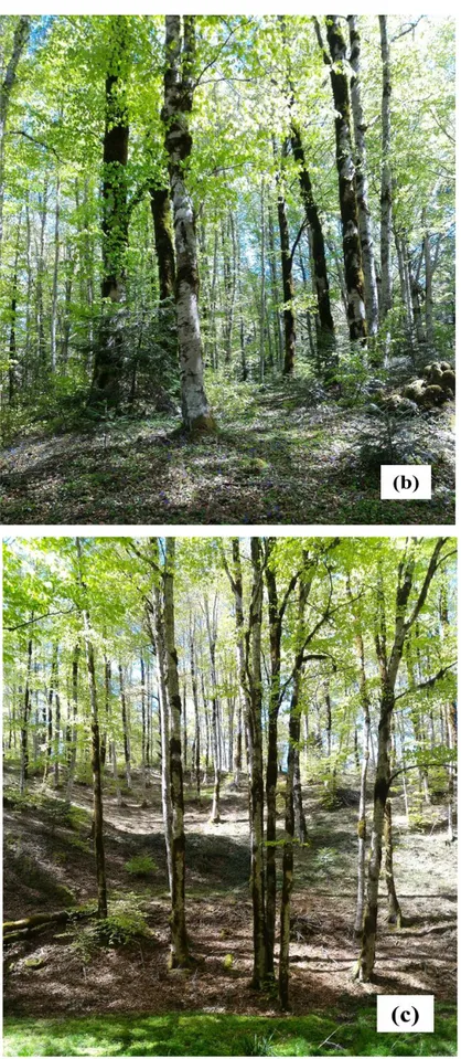
An unmanaged area for over 30 years (T1) was used as control; a traditional treatment (T2) and an innovative treatment (T3) have been carried out in 2012-2013. Traditional treatment (Fig. 5b; Fig. 6) was a thinning from below with a moderate intensity which removed all the dominated trees and the worst dominant trees (on average, ca. 12% of total volume resected). The innovative treatment (Fig. 5c; Fig. 6) was oriented to retain the 50 best trees per hectare and improve the structural biodiversity, collecting 5 or 6 trees closer to them, regardless of their social position (on average, ca. 27% of the total volume removed).

26

Fig. 5 Forest conditions at the time of the first soil sampling (2017) in: (a) control (T1); (b) traditional treatment (T2); (c) innovative treatment (T3).

27

Before the silvicultural interventions the dendrometric parameters didn’t show significant differences among the plots (Picchio et al., 2016) (Table 3).

Fig. 6 Situation before and after thinning in: (T1) traditional and (T2) innovative area

28

Table 3 Main dendrometric characteristics (± standard deviation), before and after

thinning. T1 (control), T2 (traditional), T3 (innovative) treatments. (ManFor C.BD.; Coletta et al., 2017).

The managed area are fully comparable in terms of slope, orientation and soil types. The unmanaged area (T1) was used as reference location for 137_{Cs analysis. The}

reference value obtained in this area was used to convert the 137Cs inventories obtained in the managed area into estimates of soil erosion. More specifically, the Diffusion and Migration Model (DMM) was applied for this conversion analysis (see Porto et al., 2003). This version of the DMM is based on a simulation of 137Cs activity along a soil profile following the atmospheric fallout and its temporal redistribution. Based on this assumption, the DMM attempts to reproduce the activity of 137Cs with the following equation:           













C (x,t,t’) (Bq kg-1_{) indicates the} 137_{Cs activity at the mass depth x and time t’;}

I (t’) expressed in (Bq m-2 _yr-1_{) indicates the} 137_{Cs amount received by the soil surface at}

time t’ with fallout;

Treatment Volume (m3 _ha-1₎ Basal area (m2 _ha-1₎ No. tree (N ha-1₎ T1 - 432.9 ± 174.1 38.5 ± 11.4 334 ± 201.2 T2 Before 345.7 ± 19.8 34 ± 1.2 557 ± 138.7 After 301.6 ± 15.6 29.7 ± 1 501 ± 111.5 T3 Before 338.1 ± 27.7 33.9 ± 1.9 631 ± 104.4 After 246.1 ± 21.3 26.6 ± 1.6 533 ± 94.3

29

H (kg m-2_{) is a basic parameter that accounts for the initial relaxation mass depth;}

D (kg2 m-4 yr-1) is a model parameter that simulates the diffusion process; V (kg m-2 yr-1) is a model parameter that accounts for migration;

λ (= 0.023 yr-1_{) is the constant of radioactive decay for} 137_Cs;

x (kg m-2) indicates the cumulative mass depth;

t (yr) is the time elapsed since the commencement of fallout in 1954; erfc(u) is the error-function complement defined as (Crank, 1975):

    u y dy e u erfc( ) 2 2  (2)

Integrating Eq. (1) over time t’ and assuming a continuous input I (t’), the 137_Cs

concentration C (x,t) (Bq kg-1) in the soil profile is given by the following equation:





Assuming a constant soil lowering E (kg m-2), if the transport is purely diffusional, eq. (1) can be rewritten as:

         





where, the value of Ce(x,t,t’) (Bq kg-1) indicates the concentration of 137Cs in the

presence of erosion, for any cumulative mass depth x and time t’.

The attempt of Eq. (1) to simulate the diffusion and migration of 137Cs along the soil column was demonstrated in works carried out in southern Italy by Porto et al. (2004, 2016).

In other words, integration of C(x,t) over mass depth x gives the total 137_{Cs inventory A} u

(Bq m-2_{) for an erosion site at time t:}

A_u(t) C_e(x,t) dx

0



 (5)

Eqs. (4) and (5) can then be solved simultaneously for E (kg m-2), with Au (Bq m-2)

30

(kg m-2 _yr-1_{) may then be estimated by dividing the quantity E by the time t-t}

0 (yr) since

the commencement of 137Cs fallout.

2.2 Soil sampling and preparation

For each of the three study area (T1, T2 and T3), 3 representative plots (1000 m2 _in

size) were established for soil sampling (see Fig. 4). In these 9 plots, five separate soil sampling were undertaken in two different years (2017-2018) following the scheme illustrated in Fig. 7. The first and the second soil sampling were carried out in May 2017 and consisted of collecting soil cores for 137Cs analysis separate from soil collected for chemical-physical and biological analysis. The third and fourth soil sampling, were carried out in May 2018, following the same scheme of the previous year. The cores were collected in areas with similar slope avoiding sampling points close to the tree trunks in order to minimize the effect of stemflow on the final 137Cs inventories. In total, in both years, 12 composite soil cores were obtained from these sampling campaigns (6 for radiometric measurements and 6 for chemical-physical and biological analysis), using a 10-cm-diameter steel core tube inserted up to a depth of ca. 35 cm. Each composite core used for 137Cs analysis was obtained from 9 single sectioned cores for each year (3 for each plot of the same treatment) merged layer by layer (see merging strategy explained in Fig. 7).

31

Fig. 7 Sampling strategy adopted in the plots established within the three treatment

areas.

More specifically, for each study area, the 9 single cores were sectioned into depth increments of 2-3 cm to a depth of 30 cm, and the deepest 5 cm were merged into one single sub-sample. This sampling strategy was necessary to obtain the distribution of

137_{Cs activity along the soil profile and to account for microscale variability. Each}

profile was used to fit the theoretical conversion model (DMM) able to calculate soil erosion rates.

Each composite soil core used for the chemical-physical and biological analyses consisted of 9 single soil cores (for each year), divided into 2 layers (0-15 and 15-30 cm). The corresponding layers were merged in order to obtain 3 final representative cores (one for each study area).

The fifth samplings, undertaken ever in May 2018, was necessary to further account for microscale variability associated with the 137_{Cs inventories at the reference area. These}

samplings provided collection of bulk cores from the three plots (T1a,b,c) within the

control area (T1). In order to check the 137_{Cs reference value obtained during both the}

32

comparison (see Fig. 7 for details). For the determination of microbial biomass, the samples were stored in the refrigerator at 4 ° C for up to 24 hours before being analysed. All the others samples, were air dried and sieved to separate the < 2 mm fraction. Before the radiometric assay, all the samples were oven dried at 105 °C for 48 h, disaggregated, dry sieved to separate the < 2 mm fraction, and packed in plastic pots or Petri dishes for subsequently determination of its 137Cs activity by gamma spectroscopy. For QBS-ar (microarthropods) one soil sample were taken from each of 9 plots differently managed (in both years), including the control area. The samples were taken at a depth of 10 cm. Immediately upon returning from the field, the soil samples were transferred to Berlese-Tullgren funnels lined with 4 mm wire mesh, until complete extraction.

2.3 Radiometric method for measuring 137_{Cs activity in soil}

The measurements of the 137_{Cs activity and its subsequently vertical distribution in the}

soil profile were obtained by gamma spectrometry at the Department of Agraria of the University Mediterranea of Reggio Calabria. Two Canberra p-type HPGe detectors, model GX4020, were used for the analyses. Each detector, coupled to a Desktop Spectrum Analyzer DSA-1000 Canberra multichannel analyser, is characterised by a relative efficiency of 45.6% with a resolution of 1.1 keV at 122 keV and 2.0 keV at 1.33 MeV. The spectral analysis was provided by the Canberra Genie 2000 software package and the efficiency calibration was obtained by the Canberra’s LabSOCS (Laboratory SOurceless Calibration Software) code. A certified multigamma source with a wide energy range (42.8–1274.5 keV) together with several standard materials of different geometry were used for energy calibration. Count times in the detectors were approximately 40,000 s, and the 137Cs activities were obtained from the counts at 662 keV.

33

2.4 Soil physical and chemical property determination

The Water Content (WC) was determined in according to the “Official Methods of Chemical Soil Analysis” (DM, 13/09/1999). The method covers the determination of the moisture content of a soil as a percentage of its oven-dried weight, up to a constant weight (65°C for 72 hours).

Samples of soils were analysed to determine the size distribution of the mineral particles (texture). The texture was measured using the method of Bouyoucos (1962). This method is based on Stoke’s law, governing the rate of sedimentation of particles suspended in water. The Bouyoucos method consisted of the destruction of the SOM with hydrogen peroxide and its further dispersion with sodium hexametaphosphate (Calgon). The SOM was destroyed in a 50 g soil sample by applying successive aliquots (approximately three times) of 40 mL of hydrogen peroxide (H2O2, 130 volumes) until

the effervescence of the reaction was minimal. Dispersion was obtained by shaking 50 g of dry soil sample with 100 mL of 25% sodium hexametaphosphate (technical Calgon) in a reciprocating shaker. The mixture was then placed in a Bouyoucos’ blender cup and stirred for two minutes with an electrical mixer. The contents of each cup were transferred to a 1 L sedimentation cylinder, and the cylinder was filled with deionized water to the 1000 mL mark. The mixture was then homogenized using manual agitation. Immediately after the cylinder was placed on the table and the hydrometer was gently inserted into the suspension. The solids in the suspension were measured with a hydrometer following 4 minutes of decantation with a second lecture taken after 24 hours. The measurement was made when the suspension was between 20 and 22 °C and then corrected due to the temperature. The first reading was for estimating the silt content whereas the second one at 24 hours was to estimate the clay. A soil texture triangle was used to determine the texture category. Results are reported as percentages of the mineral fraction, % sand, % silt, and % clay.

The acidity, neutrality or alkalinity of a soil are generally measured in terms of hydrogen ion activity of the soil water system. This method is essentially based on the measurement of potential, developed across an indicator or the glass electrode on account of the difference activity of H+ ions in and out of the electrode, i.e., in the bathing solution. pH in H2O was measured according to the “Official Methods of

34

glass beaker and were mixed with 25 mL H2O deionized to determine the active acidity

of soil. The suspensions were shaken for 2 hours, and after decantation, the electrode of pH-meter was immersed into the samples. The pH range normally found in soils varies from 3 to 9.

Electrical conductivity (EC) was detected according the method described by Blakemore et al. (1987): 10 g of dry soil were weighed, into a glass beaker and mixed with 50 mL H2O deionized, the suspension was shaken for 30 minutes and after

decantation the conductivity was measured by using a conductimeter.

Total nitrogen (N) was detected by Kjeldahl method (Kjeldahl, 1883). The method consists of heating soil with sulphuric acid, which decomposes the organic substances by oxidation to liberate the reduced nitrogen as ammonium sulphate. In this step potassium sulphate is added to increase the boiling point of the medium (from 337 °C to 373 °C). Chemical decomposition of the sample is complete when the initially very dark-coloured medium has become clear and colourless. The solution is then distilled with a small quantity of sodium hydroxide, which converts the ammonium salt to ammonia. The amount of ammonia present, and thus the amount of nitrogen present in the sample, is determined by back titration. The end of the condenser is dipped into a solution of boric acid. The ammonia reacts with the acid and the remainder of the acid is then titrated with a sodium carbonate solution by way of a methyl orange pH indicator. The organic carbon (OC) was detected by treating the soil with potassium dichromate and sulfuric acid, while the difference in FeSO4 added with respect to a blank titration

determined its quantity (Springer and Klee, 1954). The percentage carbon is given by the formula:

𝐶𝑂 % = 𝑀 (𝑉1 − 𝑉2 𝑊) ∗ 0.3 ∗ 𝐶𝐹 (6)

where M is the molarity of the FeSO4 solution (from blank titration), V1 is the volume

(mL) of FeSO4 required in blank titration, V2 is the volume (mL) of FeSO4 required in

actual titration, W is the weight (g) of the oven-dried soil sample and CF is the correction factor. The CF is a compensation for the incomplete oxidation and is the inverse of the recovery. This CF was set by Walkley and Black (1934) to 1.72 (recovery of 76%).

35

Total water-soluble phenols (WSP) were measured by using the Folin–Ciocalteau reagent, following the Box method (1983). Tannic acid was used as standard and the concentration of water-soluble phenolic compounds was expressed as tannic acid equivalents (μg TAE g-1 _{D.W.). 10 g dry-soil were weighed, into a conic flask and, were}

mixed with 50 mL H2O deionized, the suspensions were shaken for 24h, and then

centrifuged at 5000 rpm for 10 min. 1000 μl of Folin-Ciolcateu reagent and 2.5 mL of sodium hydroxide (0.33 N) were added to the different extracts (500 μl). The mixtures were incubated for 15 min at room temperature. The specific absorbance was immediately measured at 760 nm.

For the measurement of dissolved organic carbon (DOC), 1 gr of air-dried and 2 mm sieved soil was taken. An extraction was carried out in 10 ml of ultrapure water (1:10), after 24 hours of rest and 2 hours of shake, centrifugation was carried out at 3000 rpm for 15 minutes. The supernatant filtered with 0.45 mm cellulose acetate membrane filters, and the absorbance of the samples at 254 nm was measured with a Plate reader (Perkin Elmer Enspire) according to the method described in Brandstetter et al. (1996). Soil samples were extracted with bidistilled H2O, respectively, at a 1:10 ratio, for 24

hours at room temperature. The extract was subjected to centrifugation and the supernatant, after filtration on 0.22 μm cellulose filters, was analysed for the qualitative and quantitative determination of ions (Wang et al., 2013). The analysis was conducted using a Dionex ICS-1100 ion chromatograph. The data are reported in mg/g of dry sample.

2.4.1 Soil aggregate fraction analysis

Soil aggregate stability (SAS) by wet sieving was determined according to ON L 1072 (2004). With this method, soil aggregates with a diameter of 2000–1000 μm are dipped on a sieve of 250 μm. The mass of soil (EW) used in the experiment is 4 g. The mass of stabile aggregates after dipping (mK) in 80 ml of distilled water and the mass of sand after chemical dispersion (25 ml of sodium pyrophosphate) of the remaining aggregates (mA) is determined. These parameters are used to calculate the percentage of stabile aggregates (% SAS):

36

%𝑆𝐴𝑆 = 𝑚𝐾−𝑚𝐴

𝐸𝑊−𝑚𝐴× 100 (7)

Through the USAS method, measurable ultrasonic energy was applied to the soil-water suspension, allowing a quantitative measurement of soil aggregate stability (Mentler, 2001). The most important parameter to describe the particle dispersion during sonification and the degree of aggregate breakdown, is the specific ultrasonic energy absorbed by a soil–water mixture. Soil aggregate distribution (USAS) was carried out by a new, probe-type dispersion equipment (cite). A titanium alloy probe is inserted into the soil–water mixture and vibrates at approximately 20 kHz. The ultrasonic titanium probe has cylindrical shape and a circular cross section (diameter 30 mm). The same ultrasonic probe was used in all experiments and the insertion depth was kept constant at 10 mm.

Dispersion experiments were performed with 4 g soil in 200 ml pure degassed water. The solution was stirred with a magnetic stirring device (2 Hz, cylindrical shape with length 25 mm and thickness 8 mm). Stirring starts 10 s prior to the ultrasonic vibration and was continued during the ultrasonic experiments to obtain a homogeneous distribution of soil in the solution. All soils were tested at constant vibration amplitude of the ultrasonic probe of 2.5 μm for 30 seconds. As reported in literature (Mayer et al., 2002; Mentler et al., 2004), the vibration amplitude was determined using electromagnetic induction coil and strain gauges. Immediately after the ultrasonic treatments, mass fractions were determined by wet sieving. The aggregates were analysed with standard sieves and classified in different aggregate fractions: macro-aggregates (1000–630 µm), medium macro-aggregates (630–250 µm), and small macro-aggregates (250–63 µm). Determination of mass fractions (accuracy 0.001 g) was performed by weighing after drying at 105°C for 24 h. Each aggregate fraction was used to determination of OC and N, using an elementary analyzer via dry combustion technique and gas chromatographic analyses (ThermoFisher Flashsmart, ON L 1080-99 (1999)).

37

2.5 Soil biological and biochemical analysis

Soil microbial biomass carbon (MBC) was detected following the method of Vance et al. (1987): 5 g of each soil were fumigated with ethanol-free chloroform for 24 h at 25 °C in a sealed desiccator in the dark. 5 g of non-fumigated soil for each sample, were stored at 8 °C during this period. The next day, after removing the beaker with chloroform, the desiccator was evacuated six times to remove the chloroform from the soils. Both fumigated and non-fumigated samples were extracted with freshly prepared 0.5 M K2SO4 at 1:4 ratio and filtered. Dissolved organic carbon in all filtrates was

determined after dichromate digestion by titrating with acidified ferrous ammonium sulphate. Biomass C is the difference between C extracted from the fumigated and non-fumigated treatments, both expressed as μg C g-1_{. Finally the result was divided for 0.45}

to convert the chloroform-labile C pool to the microbial biomass C (Beck et al., 1997). Fluorescein diacetate hydrolase (FDA) activity was determined according to the methods of Adam and Duncan (2001). To 2 g of soil (fresh weight, sieved <2 mm) 15 mL of 60 mM potassium phosphate pH 7.6 and 0.2 mL 1000 mg FDA mL-1 were added. The flask was then placed in an orbital incubator at 30 °C for 20 min. Once removed from the incubator, 15 mL of chloroform/methanol (2:1 v/v) was added to terminate the reaction. The content of the flask was centrifuged at 2000 rpm for 3 min. The supernatant was filtered and the filtrates measured at 490 nm on a spectrophotometer (Shimadzu UV–vis 2100, Japan).

Dehydrogenase (DHA) activity was determined by the method of von Mersi and Schinner (1991). Dehydrogenase assays based on the reduction of 2, 3, 5- triphenyltetrazolium chloride (TTC) to the creaming red-colored formazan (TPF), have been used to determine microbial activity in soil. In each tube was added 1 ml of TTC, except for the control, which received water instead. After the addition, of water, substrate and TTC were simultaneously mixed through the soil with a sterile glass rod; then rubber stoppers were inserted, and the tubes were incubated at 37°C at 24h. Upon completion of incubation, the tubes were extracted immediately. Each soil sample was transferred with methanol to a funnel containing Whatman no. 5 filter paper. The red methanolic solutions of the formazan were read at 485 nm against the extract from the non-TTC soil blank by using a spectrophotometer (Shimadzu UV–Vis 2100, Japan).