Alma Mater Studiorum
Università di Bologna
Facoltà di ingegneria
C
ORSODI
L
AUREAIN
I
NGEGNERIAPER
L
’A
MBIENTEE
IL
T
ERRITORIOIndirizzo Tecniche e
Tecnologie Ambientali
T
ESIDI
L
AUREAIN
M
ICROBIOLOGIAE
B
IOTECNOLOGIEA
MBIENTALIINTERACTIONS OF PLANTS AND BACTERIA IN
PCBCONTAMINATED SOILS – NATURAL WAYS
FOR REMOVAL OF POLLUTANTS
TESI DI LAUREA DI: RELATORE: FEDERICO STRACCIA Chiar.mo Prof. FABIO FAVA CORRELATORI: Prof. MARTINA MACKOVA Dr. ONDREJ UHLÌK SESSIONE IIIANNO ACCADEMICO 20082009
Keywords
Rhizoremediation
PCB
Bioremediation
Phytoremediation
Pseudomonas
JAB1
Contaminated soil
Dedicated to Elena who waited so long, to her love which supported me. To my family which allows me to travel. To colleagues from ICTPrague and their precious help. Real friends, thank you
Index
1. INTRODUCTION...4 1.1 PCBs' nature and characteristics...4 1.1.1 Physical and chemical properties...4 1.1.2 Commercial mixtures...5 1.2 PCBcontaminated sites...6 1.2.1 Contamination in Europe...6 1.2.1 Contamination in Italy...7 1.3 Remediation techniques...8 1.3.1 Physical treatments...8 1.3.2 Chemical treatments...9 1.3.3 Microbial treatments...9 1.3.4 Remediation techniques in Europe...11 1.3.5 Remediation techniques in Italy...12 1.4 Rhizoremediation of PCBcontaminated sites...13 2. MATERIALS & METHODS...14 2.1 Materials...14 2.1.1 Plants...14 2.1.2 Soil...14 2.1.3 Chemicals...16 2.1.4 Bacterial strain JAB1...18 2.2 Methods...18 2.2.1 Plant's cultivation and soil augmentation...18 2.2.2 PCB extraction from soil for PCB analysis...19 2.2.3 Plate counting...20 3 RESULTS...27 3.1 Analysis of cultivable bacterial populations by plate counting...27 3.1.1 The beginning of the experiment...27 3.1.2 The end of the experiment...293.1.3 Comparison of the results of total counts of microbes at the beginning and at the end of experiment...31 3.2 Chemical analysis...34 3.3 Toxicity tests...46 3.3.1 Contact test (soil)...46 3.3.2 Contact test (water)...48 3.3.3 Vibrio fischeri...50 3.4 DNA Analysis...55 3.4.1 DNA isolates from agar plates...55 4 CONCLUSIONS...56 4.1 Introduction...56 4.2 Scoping...56 4.3 Experiment's results...56 5 REFERENCES...58
1. INTRODUCTION
1.1 PCBs' nature and characteristics
Polychlorinated biphenyls (PCBs) are a class of organic compounds with one to ten chlorine atoms attached to biphenyl, which is a molecule composed of two benzene rings (Figure 1). The chemical formula for PCBs is C12H10xClx, where x = 1,2,...,10. Figure 1: Polychlorinated biphenyls' general chemical formulaPCBs were widely used for many applications, especially as dielectric fluids in transformers, capacitors, and coolants.
1.1.1
Physical and chemical properties
PCB congeners are odorless, tasteless, clear to paleyellow, viscous liquids (the more highly chlorinated mixtures are more viscous and deeper yellow). They are formed by electrophilic chlorination of biphenyl with chlorine gas. Theoretically 209 different PCB congeners are possible (Snell et al., 2007), although only about 130 are found in commercial PCB mixtures (UNEP Chemicals, 1999). PCBs have low water solubilities and low vapor pressures at room temperature, but they have high solubilities in most organic solvents, oils, and fats. They have high dielectric constants, very high thermal conductivity, high flash points (from 170 to 380°C) and are chemically fairly inert, being extremely
resistant to oxidation, reduction, addition, elimination, and electrophilic substitution (Boate et al., 2004). The density varies from 1.182 to 1.566 kg/L.Other physical and chemical properties vary widely across the class. As the degree of chlorination increases, melting point and lipophilicity increase, but vapour pressure and water solubility decrease (UNEP, 1997). PCBs readily penetrate skin, PVC (polyvinyl chloride), and latex (natural rubber). PCBresistant materials include Viton, polyethylene, polyvinyl acetate (PVA), polytetrafluoroethylene (PTFE), butyl rubber, nitrile rubber, and Neoprene.
1.1.2
Commercial mixtures
Commercial PCB mixtures were marketed under different names (Table 1) (Japan Offspring Fund, 2003). Due to PCB's toxicity and classification as persistent organic pollutants, PCB production was banned by the United States Congress in 1979 and by the Stockholm Convention on Persistent Organic Pollutants in 2001. Producer countries Name of PCB mixture Brazil Ascarel Former Czechoslovakia Delor France Phenoclor, Pyralène (both used byProdolec) Germany Clophen (used by Bayer) Italy Apirolio, Fenclor
Japan Kanechlor (used by Kanegafuchi), Santotherm (used by Mitsubishi) United Kingdom Aroclor xxxx (used byMonsanto Company), Askarel, Pyroclor
United States Aroclor xxxx (used by Monsanto Company), Asbestol, Askarel, Bakola131, Chlorextol (Allis Chalmers trade name), Hydol, Inerteen (used byWestinghouse), Noflamol, Pyranol/Pyrenol (used byGeneral Electric), SafTKuhl, Therminol Former USSR Sovol, Sovtol Table 1: Names of different PCB mixtures and respective producer country.
1.2 PCBcontaminated sites
Large PCB production and usage, and relative carelessness, resolved in wide environmental contamination. PCB contamination in the environment has come exclusively from human activities. Thus high PCB concentration areas tend to be around industrialized areas; PCBs enter the general environment mainly by leakage of supposedly closed systems, from landfill sites, incineration of waste, agricultural lands, industrial discharges and sewage effluents. High PCB's solubility into organic solvents and fats involves easy sorbtion onto soil particles, especially on the organic fraction.
1.2.1 Contamination in Europe
European recent estimates report approximately 250000 contaminated sites (3 millions potentially contaminated) but this number is expected to grow due to proceeding of monitoring and investigation activities. Industrial and commercial activities as well as disposal and treatment of wastes are the most important sources of contamination. In the last 30 years only 80000 sites were remediated (European Environment Agency, 2007). Contamination by spread or local pollution sources causes important loss of functionality of relevant agricultural and former industrial areas. Research of solutions for management and prevention of soil and groundwater pollution has become a political priority for Europe. One of the main tasks is to create national inventories of contaminated and potentially contaminated sites, potentially polluting activities, recent and historical contamination. Often informations about localization, sitespecific characteristics, environmental and health impact and site's management are provided. Since 2004 European Environment Agency works to identify contamination risk areas in european context.
PCB contaminated sites can be found in many different western and eastern european countries: United Kingdom, Norway, Former Czechoslovakia, Poland, Croatia (Holoubek, 2000), France (Motelay Massei et al. , 2003), Spain(Fernandèz et al. , 1998), Romania (Covaci et al. , 2001).
Annual national expenditure for the management of contaminated sites are on average about 12€ per capita, with a range of approximately 0.2 to more than 20€ per capita in the reporting countries (European Environment Agency, 2007).
1.2.1
Contamination in Italy
More than 15000 contaminated sites are present in Italy: more than 50 have national relevance, more than 5000 regional relevance. These sites' soil surface is 3% of the whole national territory (Amanti et al., 2008). Figure 2: Localization, size and referential law for National Interest Sites (Amanti et al., 2008). Two main PCB contaminated sites are Porto Marghera in Venice lagoon (D'Aprile, 2008; Tomiato et al., 2005) and Caffaro Chemicals industrial site close to Brescia, Lombardia (http://www.comune.brescia.it/NR/exeres/4F18B7A58A914936B7A914152CEE9253.htm). They are both industrial sites: a petrochemical refinery works in Porto Marghera; Caffaro Chemicals, petrochemical refineries too, stopped to work in 2008 after its attachment. These sites are contaminated on a big scale by PCBs and other pollutants (mineral oil, heavy metals) widely spread into sediments (Porto Marghera) and soil (Caffaro Chemicals site, Brescia) and their characterization is still under way. Due to their difficult remediation with “regular” techniques, they can be an excellent occasion to test the effectiveness of biological approaches. Sites' surface(ha) Referential law
1.3 Remediation techniques
Reclaiming of PCB contaminated sites pass through PCB's destruction, dechlorination or transformation in less toxic compounds. It may occur using different techniques which can be separated in three different categories: physical, chemical and microbial.
1.3.1 Physical treatments
Incineration: although PCBs do not ignite themselves, they can be combusted under extreme and carefully controlled conditions. The current regulations require that PCBs are burnt at a temperature of 1200°C for at least two seconds, in the presence of fuel oil and excess oxygen. A lack of oxygen can result in the formation of PCDDs (polychlorinated dibenzodioxins) , PCDFs (polychlorinated dibenzofurans) and dioxins, or the incomplete destruction of the PCBs. Such specific conditions mean that it is extremely expensive to destroy PCBs on a tonnage scale, and it can only be used on PCB containing equipment and contaminated liquid. This method is not suitable for the decontamination of affected soils (Mujeebur Rahuman et al., 2000);Ultrasound: in a similar process to combustion, high power ultrasonic waves are applied to water, generating cavitation bubbles. These then implode or fragment, creating microregions of extreme pressures and temperatures where the PCBs are destroyed. Water is thought to undergo thermolysis, oxidising the PCBs to CO, CO2 and hydrocarbons such as biphenyl, and releasing chlorine. The scope of this method is limited to those congeners which are the most water soluble; those isomers with the least chlorine substitution (Mujeebur Rahuman et al., 2000) Irradiation: if a deoxygenated mixture of PCBs in isopropanol or mineral oil is subjected to irradiation with gamma rays then the PCBs will be dechlorinated to form biphenyl and inorganic chloride. The reaction works best in isopropanol if potassium hydroxide (caustic potash) is added. Solvated electrons are thought to be responsible for the reaction. If oxygen, nitrous oxide, sulfur hexafluoride or nitrobenzene is present in the mixture then the reaction rate is reduced. This work has been done recently in the US often with used nuclear fuel as the radiation source (Mincher et al. , 1992; Mincher et al., 1998); Pyrolysis: destruction of PCBs with pyrolysis using plasma arc processes, like incineration uses heat, however unlike incineration, there is no combustion. The long chain molecules are broken with extreme temperature provided by an electric arc in an inert environment. Adequate post pyrolisis post treatment
of the resultant products is required in order to prevent the risk of back reactions (Mujeebur Rahuman et al. , 2000; ).
1.3.2 Chemical treatments
Many chemical methods are available to destroy or reduce the toxicity of PCBs. Nucleophilic aromatic substitution is a method of destroying low concentration PCB mixtures in oils, such as transformer oil (De Filippis et al. , 1999). Between 700 and 925°C, H2 cleaves the carbonchlorine bond, and cleaves the biphenyl nucleus into benzene yielding HCl without a catalyst. This can be performed at lower temperatures with a catalyst, and to yield Hcl and biphenyl (Forni et al. , 1998). However, since both of these routes require an atmosphere of hydrogen gas and relatively high temperatures, they are prohibitively expensive. The solution photochemistry of PCBs is based on the transfer of an electron to a photochemically excited PCB from a solidphase catalyst, to give a radical anion (Lores et al. , 2002).1.3.3 Microbial treatments
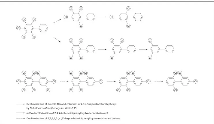
Much recent work has centered on the study of microorganisms that are able to decompose PCBs (Chekol et al. , 2004; Cunningham and Berti, 1993; Demnerova et al. , 2005; Gibson et al. , 1993; Kas et al. , 1997; Leigh et al. , 2006; Mackova et al. , 2009; Ryslava et al. , 2004). Generally, these organisms work in one of two ways: either they use the PCB as a carbon source (Figure 3), or destruction takes place through reductive dechlorination (Bedard et al., 2006; Cutter et al., 2001; Fennell et al., 2004) , with the replacement of chlorine with hydrogen on the biphenyl skeleton (Figure 4). However, there are significant problems with this approach.
Figure 3: Pathway for biphenyl degradation. BphA=Biphenyl 2,3dioxygenase; BphB=cis2,3dihydro 2,3dihydroxybiphenyl dehydrogenase; BphC = 2,3dihydroxybiphenyl 1,2dioxygenase; BphD=2 hydroxy6phenyl6oxohexa2,4dieneoate (HOPDA) hydrolase; BphH(E)=2hydroxypenta2,4 dienoate hydratase; BphI(F)=acylating acetaldehyde dehydrogenase; BphJ(G) = 4hydroxy2 oxovalerate aldolase; BCL = benzoateCoA ligase; BenABCD=benzoate 1,2dioxygenase and benzoate dihydrodiol dehydrogenase.
Figure 4: Bacterial reductive dehalogenation of selected polychlorinated biphenyls by Dehalococcoides and related bacteria and by an enrichment culture (Bedard et al., 2006; Cutter et al., 2001; Fennell et al., 2004).
Firstly, these microbes tend to be highly selective in their dechlorination, with lower chlorinated biphenyls being readily transformed, and with preference to dechlorination in the para and meta
positions. Secondly, microbial dechlorination tends to be rather slow acting on PCB as a soil contaminant in comparison to other methods. Finally, while microbes work well in laboratory conditions, there is often a problem in transferring a successful laboratory strain to a natural system. This is because the microbes can access other sources of carbon, which they decompose in preference to PCBs.
1.3.4 Remediation techniques in Europe
Monitoring and remediation techniques presently applied in Europe are phisical, chemical and biological, even though approaches most frequently adopted consist in “traditional” measures like D&D (Dig&Dump) and containment, namely approaches that consider soil like waste to dispose, not a resource to remediate and reuse (European Environment Agency, 2007).
To promote exchange of experiences between different European countries, which is the essential requirement to create an advanced and efficient remediation experience network, European Union financed various “concerted efforts”, some of them aimed to develop technical recommendations for a sustainable management and, above all, reuse of contaminated sites and sediments (SEDNET, http://www.sednet.org/ ). some other, like NICOLE (http://www.nicole.org), Common Forum for
Contaminated Land in Europe, to make ready new sustainable remediation techniques as well as
cooperation between academic and industrial world on this subject, and EURODEMO (http://www.eurodemo.info), which is aimed to collect and compare remediation technologies already successfully used in Europe, helping the promotion of the most effective in european context.
Europe is slowly moving toward coordinated approach to the big problem of environmental contamination, focusing R&D efforts in finding new and more effective toxicological and environmental risk analysis techniques, to provide a more effective and reliable characterization of real danger; implementing, optimizing and adjusting bioremediation technologies already known and available to realize effective, economical and sustainable recover of priority highrisk sites; training young researchers and technicians to make it possible.
1.3.5 Remediation techniques in Italy
Monitoring and reclamation of contaminated sites in Italy take place for the most using conventional techniques: D&D (Dig&Dump) for soils and P&T (Pump&Treat) for groundwater.
Remediation Technology State Remediation Technology State
EX SITU Dig and Dump/Treatment XXX Thermal Desorption XX Incinerating XX Soil washing XX Landfarming XXX Pump and Treat XXX Biopile XXX Immobilization X Compost XX IN SITU Physical barriers XXX Electromigration X Soil vapor extraction XXX Thermal treatment X Idraulic Fracturation X Chemical Oxydation XX Air sparging XXX Solidification/Stabilization X Bioventing XXX Groundwater Circulation Well (GCW) XX Biosparging XXX MultiPhase Extraction XXX Reductive Dehalogenation X
Permeabile Reactive Barriers XX Monitoredattenuation natural XX
Soil flushing XX Phytoremediation XX Table 2: State of application of different reclamation technologies to remediate contaminated sites in Italy; XXX=wide application; XX=some field application; X=demonstrative or pilot application. Nevertheless in the last years more frequent use of modern remediation techniques was registered; Table 2 shows reclamation techniques currently exploited in Italy to manage contaminated sites. Ex situ approaches prevail: D&D for soil and P&T for water, are characterized by low environmental sustainability because pollutants are not destroyed and the contaminated resource (soil or water) does not regain it's original or potential use. Even though improvements have been registered in the recent time, in situ approaches remain rare and to evaluate, even concerning techniques largely used in other european countries.
1.4 Rhizoremediation of PCBcontaminated sites
PCBs are very stable compounds and do not degrade readily. Their destruction by chemical, thermal, and biochemical processes is extremely difficult, and presents the risk of generating extremely toxic dibenzodioxins and dibenzofurans through partial oxidation. Their very low water solubility makes them difficult to extract into water, although water transport may occur due to sediments and soil handling (dredging, digging): that is why conventional techniques like D&D and vapour desorption are not very effective and may also contribute to spread contamination. Phytoremediation and rhizoremediation are proved to be viable in situ remediation techniques(Mackova et al. , 2009; Ryslava et al. , 2004): combined action of plants and microorganisms populating the rhizosphere, that is plant roots volume's surface, can degrade a large number of contaminants restoring chemical, physical and biological characteristics of intact soil.Different strains of PCBdegrading bacteria have already been isolated and characterized from environmental samples (Bedard et al., 1990; Denef et al., 2004; Mondello et al., 1997; Leigh et al., 2006). However the knowledge about bacteria and plants' interaction must be improved. The aim of this experiment is to find out if a PCBdegrader bacterial strain, previously isolated and cultivated at laboratory conditions to improve its PCBmetabolizing abilities, could be reintroduced in its natural environment in symbiotic relationship with specific plant. Plantbacteria interactions and effects on PCB removal were analyzed.
2. MATERIALS & METHODS
2.1 Materials
2.1.1 Plants
Six plants of Nicotiana tabacum (Figure 5) were used for this experiment, making them grow in contaminated soil and coupling them with the chosen bacterial strain. Figure 5: little plant of Nicotiana tabacum Tobacco plants were chosen because they are able to phytoaccumulate large amounts of PCBs in leaves and roots (Ryslava et al., 2003; Mackova et al., 2009) and a higher number of bacteria was revealed in comparison with other plants (Ryslava et al., 2004). Lactuca sativa seeds were used for toxicity contact test for eukaryotic organisms.
2.1.2 Soil
Soil samples were collected in 2007 from a 15yearold of PCBcontaminated soil dumpsite in Lhenice, South Bohemia. Soil is contaminated with different organic xenobiotics including PCBs represented by Delor103: it's the mixture of 60 individual PCB congeners with average of 35 chlorines per molecule. Eight pots have been filled with 450 g of polluted soil: six of them were vegetated with tobacco (Figure 7,8); two containing bulk soil only (Figure 6). Three of six pots with tobacco plants were inoculated with PCB degrading bacteria Pseudomonas sp. Strain JAB1 (Figure 8). Small amounts of soil have been collected from each pot at different depths (surface, half, bottom)around 2,5 hours after the first inoculation (initial) and one week after the last (final). Finally six different combinations of soil samples were compared after homogenization: − CONTROL(initial) and CONTROL(final) from bulk soil; − TO+CO(initial) and TO+CO(final) from soil with tobacco plants; − TO+CO+JAB1(initial) and TO+CO+JAB1(final) from soil with tobacco plants and inoculation. Figure 6: Tobacco plants in contaminated soil. Figure 7: Tobacco plants in contaminated soil augmented with Strain JAB1. Figure 8: Bulk contaminated soil
Soil from each combination was split into three parts: one for DNA isolation and plate counting (CONTROL, TO+CO, TO+CO+JAB1), one for PCB extraction and chemical analysis, and one for toxicity assessment.
2.1.3 Chemicals
Solutions Pyrophosphate solution (0.1% Na4P2O7, autoclave sterilized) has been prepared for soil extractions. Saline solution (0,85% NaCl, autoclave sterilized) has been prepared for dilutions. Basal mineral solution has been used as liquid culture medium for incubation and inoculation of bacterial strain. It's prepared as a mix of four different solutions: Solution A: • 10g (NH4)2SO4; • 27g KH2PO4; • 109,55g Na2HPO4.12H2O; • distilled water up to 1000ml; Solution B: • 0,3g Ca(NO3)2; • distilled water up to 50ml; Solution C: • 0,1g FeSO4; • distilled water up to 50ml; Solution D: • 2g MgSO4; • distilled water up to 50ml; Solutions were autoclavesterilized before to mix. In order to prepare the basal mineral solution, 100ml of solution A were mixed with 5ml of solution B, C, and D and filled with sterile distilled water up to 1000ml. Agar media Three different agar gels have been used for plate counting and bacteria's isolation :− Standard Plate Count Agar (APHA) was prepared according to manufacturer's instructions, by OXOID LTD., Hampshire, England;
− Pseudomonas Agar Base, selective for Pseudomonases, was prepared according to manufacturer's instructions, by OXOID LTD., Hampshire, England; − Minimal Medium was prepared autoclavesterilizing and mixing in the rate 1:1 solutions A and B before pouring into Petri dishes (Figure 6). Figure 9:Plastic Petri dishes. Solutions were prepared as it follows: Solution A: • 5.37g Na2HPO4.12H2O; • 1.3g KH2PO4; • 0.2g MgSO4.7H2O; • 0.5g NH4Cl; • distilled water up to 500ml; Solution B: • 18g DifcoTM Agar Noble; • distilled water up to 500ml. Agarose gel prepared (1% agar) in TBE buffer for electrophoresis. Substrates
Biphenyl crystals as sole carbon and energy source for bacterial metabolism have been added to the lid of Petri dishes with minimal culture medium (Mineral Medium, Basal Mineral Solution) to serve as the sole carbon source for bacteria.
2.1.4 Bacterial strain JAB1
Pseudomonas sp. strain JAB1 has been chosen as efficient PCB degrader for this study (Ryslava et al.,
2003). Previous studies isolated it from contaminated soil in area of previous industrial plant in Jablonne v Podjestedi, Moravia.
JAB1 strain was grown on biphenyl as sole carbon source to induce bphA dioxygenase enzyme production (Master and Mohn, 2001).
2.2 Methods
2.2.1 Plant's cultivation and soil augmentation
Six plants have been grown in pots with contaminated soil for a total period of three months watered once every three days, parasite insects presence was prevented. Tobacco plants were grown in PCB contaminated soil for 4 weeks to adapt them for the PCB content and to allow augmentation of the soil with suspensions of degrading bacteria. Bacterial cells have been incubated at 28oC while shaking (135 rpm). Inoculations were performed in a period of eight weeks, around once every two weeks: 10ml of fresh liquid cultures (35 days) were poured into three of the six pots with plants. Concentration of bacterial cells was fixed to OD around 1 obtained at =600nm wavelength. OD measured every time beforeλ augmentation of the pots: I. 1,067; II. 0,907; III. 1,700; IV. 0,963. All the plants have been harvested nine weeks later the period for adaptation (the end) and stored in the freezer inside plastic bags at 20oC. Plant's tissues (roots and leaves) and small amounts of the different soils have been exploited for PCB extraction and chemical analysis.2.2.2 PCB extraction from soil for PCB analysis
Ten samples from CONTROL(final), TO+CO(initial), TO+CO(final), TO+CO+JAB1(initial), TO+CO+JAB1(initial) soils each and nine from leaves and roots of plants cultivated in augmented and non augmented soils were prepared according to the following protocol: 1. Dry plant's leaves and roots were milled and homogenized; the same was performed with different soils. Samples of dry soil and plant's tissues were sieved through sieve with diameter 1×1 mm. Soil and plants were dried in the oven at temperature to 50 °C; 2. 0,1g of soil and plant's tissues were weighted with analytical accuracy and weights put into 8ml vials. Weight was assessed to 4 decimal places. Samples were prepared the day before extraction performed. It is possible to store samples at laboratory temperature. Vials were closed tightly with teflon line septa; 3. Exactly 5ml of waterless diethylether GC grade was added to each sample. Work in the hood. Vials were closed tightly and placed into horizontal shaker; 4. Samples were taken after 6 hours of shaking, filtered into 1,5 ml vials through pasteur pipette containing Florisil. Prepared samples were closed tightly with teflon lined septa with cap and placed into the freezer (4 °C is enough); 5. Measurement was performed at these conditions: the PCBs were extracted with the diethylether. Concentration of PCBs from diethylether was provided on gas chromatograph (HP 6890N) with automatic injector (HP 7683) and a microelectron capture detector. PCB congeners were separated on a capillary column (DBXLB, length 30m, inside diameter 0,25 mm and thickness of stationary phase 0,25 μm). The mobile phase was nitrogen and the final flow was 45,1 ml/min. Samples (1 μl) were injected on column using splitless technique.
Measurement was carried out in the isobaric mode (0.993 bar). The temperature program was following: the initial temperature was 50 °C and immediately increased to 160 °C (rate 30 °C/min) and then immediately increased to 300 °C (rate 2,5 °C/min) and then terminated. Detector temperature was 340 °C and final flow of mobile phase was 60 ml/min (makeup gas + column flow). Data were collected and analyzed by using GC ChemStation software version B.03.02.
2.2.3 Plate counting
Agar media and soil extracts were used in order to study changes in microbial population and isolate the studied strain according to the following protocol: − homogenize each soil sample; − make soil extract mixing 10g soil with 90ml 0,1% Na4P2O7 solution in 250ml Erlenmayer flasks (Figure 8); incubate at 28C for 2 hours (exactly!) while shaking (130 RPM); − mix 5 ml of the soil extract with 45 ml saline solution in a Falcon tube (Figure 9); − make a series of dilutions by mixing 0.5 ml of the extract from the previous step with 4.5ml physiological solution in a testtube; − inoculate 100 μl on plates (Figure 7) according to figure (2 replicate plates for each dilution) 100 MO/g soil 101 MO/g soil 103 MO/g soil 104 MO/g soil 105 MO/g soil 106 MO/g soilsoil in Na4P2O7 45 ml 4.5 ml 4.5 ml 4.5 ml 4.5 ml
0.85% NaCl 0.85% NaCl 0.85% NaCl 0.85% NaCl 0.85% NaCl
104 MO/g soil 105 MO/g soil 106 MO/g soil 107 MO/g soil
− count the colonies after 1, 2 (PCA) and 4, 5 (MM) days of cultivation at 28oC. MM PSA MM PSA PCA MM PSA PCA PCA ...
Figure 10: Agar plates. Figure 12: 50ml Falcon tube and 15ml test tube. Biphenyl crystals added as sole carbon and energy source for bacterial metabolism to MM agar plates. Mineral medium has been used to isolate PCBdegrading strains. Two parallels A and B prepared for each soil suspension in pyrophosphate solution to have greater accuracy. Isolates collected from MM 104 MO/g soil plates have been exploited for DNA isolation, amplification by PCR (Polymerase Chain Reaction), and analysis by electrophoresis. Figure 11: 250ml Erlenmayer flask.
2.2.4 DNA isolation and amplification
Samples have been obtained in the following way: − pour 2ml of basal mineral solution on the agar plate; − scratch away the colonies from the surface with a sterile glass wand; − recollect colonies pipetting the obtained solution in 1,5ml Eppendorf vials. Twelve samples have been obtained (one each plate) and stored into the freezer at 20oC. DNA isolation has been performed with QIAmp® DNA Mini Kit (Figure 10), following protocol forisolation of genomic DNA from bacterial plate cultures (QIAmp® DNA Mini and Blood Mini
Handbook, Appendix D: Protocols for Bacteria). Figure 13: QIAmp® DNA Mini Kit. Obtained DNA solutions were exploited for PCR (Polymerase Chain Reaction) 16S. Six samples were made from the solutions: one from each of different soil sample, one positive control, one negative control. The negative control is solution without DNA; pure bphA DNA was used for positive control. Pipetting performed in sterile conditions avoiding creation of bubbles. The presence of JAB1 strain among the isolates was verified by PCR amplification of a portion of bphA gene. The primers targeting this gene were designed using MEGA4 software according to the
database (http://fungene.cme.msu.edu/) so that the primers target only the bphA genes in JAB1. However, some closely related strains, such as P. pseudoalcaligenes KF707, have very similar genes and the designed primers may have targeted bphA in other pseudomonads (Iwai S. et al. , 2010). Samples had the following composition: μl WATER 20,4 BUFFER 2,5 dNTPs (10mM) 0,5 PRIMERS (100μM) 0,05 BSA (Bovin Serum Albumin) 0,25 POLYMERASE 0,25 DNA 1 (0,25x4) TOTAL 25 Table 1: PCR samples composition. The process was performed in five steps: 1) 95oC, 5min; 2) 95oC, 45s; 3) 59oC, 45s; 4) 72oC, 1:30min; 5) 72oC, 10min. Steps three to five were repeated 35 times; 34 cycles were performed.
2.2.5 DNA analysis
Gel electrophoresis was performed to investigate bphA gene DNA presence in plate's samples, according to the following protocol: − prepare agarose gel; − add ethidium bromide in concentration of 1μl EB/30ml gel; − prepare vaults' content: 1kB ladder (better 100B ladder for bphA DNA), 5x2μl load dye + 5μl DNA. Electrophoresis was performed at 110V.
2.2.6 Toxicity tests
Contact test (soil)
The aim of this test was to investigate toxicity of soil for eukaryotic organisms: Lactuca sativa L. var.
capitata L. was the test organism.
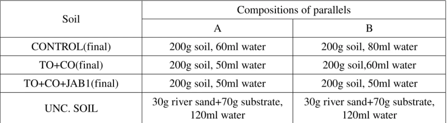
Eight parallels in closed plastic boxes were prepared: two (A,B) each different contaminated soil (CONTROL, TO+CO, TO+CO+JAB1) plus two (A,B) with uncontaminated soil. Water has been poured in each parallel little by little until soil was wet but not muddy (different amounts of water depending on soil's type).
Soil Compositions of parallels
A B
CONTROL(final) 200g soil, 60ml water 200g soil, 80ml water TO+CO(final) 200g soil, 50ml water 200g soil,60ml water TO+CO+JAB1(final) 200g soil, 50ml water 200g soil, 50ml water
UNC. SOIL 30g river sand+70g substrate, 120ml water 30g river sand+70g substrate, 120ml water
Table 2: Contact test soil samples; CONTROL(final)= contaminated bulk soil at the end of experiment; TO+CO(final)= vegetated soil at the end of experiment; TO+CO+JAB1(final)= augmented soil at the end of experiment; UNC. SOIL= commercial available river sand and soil substrate; A,B= samples' parallels.
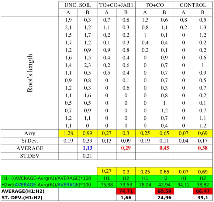
15+2 Lactuca sativa seeds were posed in three lines 0,51 cm deep in the soil then boxes were closed with parafilm and put into the incubator at 22oC. Roots' length was measured after four days, toxicity's
values were calculated using lengths according to the formula:
Relative toxicity=
UNC . SOIL root's average length
−
Soil root'saverage length
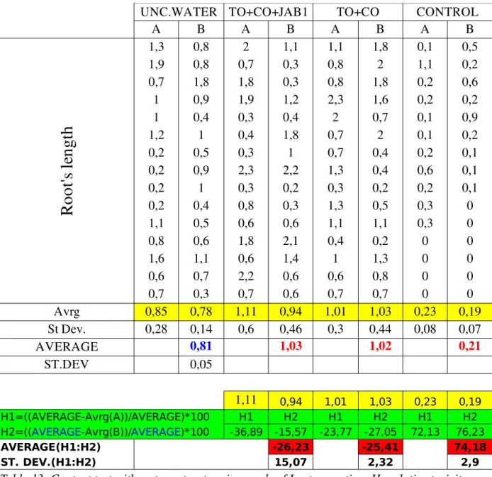
UNC . SOIL root's average length ×100Contact test (water) The aim of this test was to investigate toxicity of water extract from soil for eukaryotic organisms: Lactuca sativa L. var. capitata L. was the test organism. Eight parallels in closed glass Petri dishes were made: two (A,B) each different contaminated water (CONTROL, TO+CO, TO+CO+JAB1) plus two (A,B) with uncontaminated control solution. Water extracts were obtained as it follows: − suspend 10g of soil in 100ml of water in 250ml Erlenmayer flasks; − shake for 24 hours (135rpm, 28oC); − pour 10ml of the suspension in three Falcon tubes each;
− separate solid and liquid phases by centrifuging tubes (5000rpm, 3min, temperature not specified). Two tubes with water were exploited for contact test, one for Vibrio fischeri test. Bottom of glass Petri dishes was covered with two layers of filter paper; 10ml of water from one tube have been poured over the paper of one dish (each tube was used for only one dish). Water Extract Extract amount in parallel A B CONTROL(final) 10ml 10ml TO+CO(final) 10ml 10ml TO+CO+JAB1(final) 10ml 10ml UNC. SOLUTION 10ml 10ml Table 3: Contact test water samples; CONTROL(final)=water extract from contaminated bulk soil at the end of experiment; TO+CO(final)= water extract from vegetated soil at the end of experiment; TO+CO+JAB1(final)= water extract from augmented soil at the end of experiment. 15+2 seeds were posed on the paper, then Petridishes were closed and covered with tin layers to exclude the effect of light and put in the incubator at 22oC. Roots' length was measured after four days, toxicity's values were calculated using root lengths according to the formula:
Relative toxicity=
UNC . SOLUTION average length
−
Water Extract average length
UNC . SOLUTION average length ×100
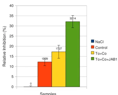
Luminescence test The aim of this test was to investigate toxicity of water extract from all soil versions to prokaryotic organisms. A working suspension of luminescent bacteria was prepared by reconstituting a vial of lyophilized cells of Vibrio fisheri, using 0.5ml of 2% NaCl aqueous solution at 25oC. The bacterial suspension was added to 0.5ml dilution series of toxicants (ZnSO4, water extracts from soil samples) in 2% NaCl. Luminescence was measured after 15 minutes incubation at 15oC. Toxicity was calculated according formula: H=
1− I Iref
⋅100 H=relative inhibition of luminescence [%] I=intensity of light produced by indicator bacteria in test tube with tested sample of soil extract Iref=intensity of light produced by indicator bacteria in presence of control nontoxic water extract3 RESULTS
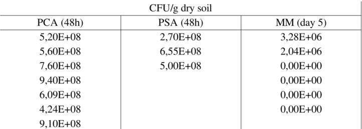
3.1 Analysis of cultivable bacterial populations by plate counting
Counts of microbial colonies grown on agar plates were performed at the beginning and the end respectively, considering the number of colonies as CFU (Colony Forming Units), in order to study changes in microbial populations and to detect and isolate the studied strain. Bacterial colonies grown on PCA and PSA plates were counted after 12 days; MM plates were counted after 45 days. Average, standard deviation and total count (Tables 7, 11) were calculated on refined data (Tables 4, 5, 6, 8, 9, 10); raw data are shown in the Appendix (Tables 16 to 21).3.1.1 The beginning of the experiment
CFU/g dry soil
PCA (48h)
PSA (48h)
MM (day 5)
9,56E+08
0,00E+00
1,14E+06
9,00E+08
0,00E+00
4,48E+06
1,44E+09
0,00E+00
8,00E+05
8,10E+08
0,00E+00
2,50E+06
9,60E+08
0,00E+00
3,60E+06
1,06E+09
0,00E+00
3,36E+06
7,20E+08
0,00E+00
6,00E+05
0,00E+00
0,00E+00
0,00E+00
Table 4: Total counts of microorganisms in CONTROL=contaminated bulk soil, beginning; PCA=Standard Plate Count Agar; PSA=Pseudomonas Selective Agar; MM=Minimal Medium; CFU=Colony Forming Units.CFU/g dry soil
PCA (48h)
PSA (48h)
MM (day 5)
5,20E+08
2,70E+08
3,28E+06
5,60E+08
6,55E+08
2,04E+06
7,60E+08
5,00E+08
0,00E+00
9,40E+08
0,00E+00
6,09E+08
0,00E+00
4,24E+08
0,00E+00
9,10E+08
Table 5: Total counts of microorganisms in TO+CO=contaminated vegetated soil, beginning; PCA=Standard Plate Count Agar; PSA=Pseudomonas Selective Agar; MM=Minimal Medium; MM=Minimal Medium; CFU=Colony Forming Units.CFU/g dry soil
PCA (48h)
PSA (48h)
MM (day 5)
1,13E+08
1,39E+08
2,36E+06
9,12E+07
6,84E+07
2,64E+06
1,61E+08
2,26E+08
1,40E+06
1,72E+08
1,54E+08
2,10E+06
1,52E+08
1,66E+08
2,80E+06
3,40E+08
2,19E+08
1,00E+06
2,47E+08
8,70E+07
2,00E+06
3,30E+08
2,56E+08
2,00E+06
2,00E+06
Table 6: Total counts of microorganisms in TO+CO+JAB1=contaminated augmented soil, the beginning; PCA=Standard Plate Count Agar; PSA=Pseudomonas Selective Agar; MM=Minimal Medium; CFU=Colony Forming Units
CFU/g dry soil
PCA (48h) PSA (48h) MM (day 5) CONTROL
Average 9,78E+08 0,00E+00 2,35E+06
St. Dev. 2,32E+08 0,00E+00 1,53E+06
Total count 5,41E+09 0,00E+00 1,65E+07
TO+CO
Average 6,75E+08 4,75E+08 8,87E+05
St. Dev. 1,99E+08 1,94E+08 1,43E+06
Total count 4,72E+09 1,43E+09 5,32E+06
TO+CO+JAB1
Average 2,01E+08 1,65E+08 2,03E+06
St. Dev. 9,46E+07 6,67E+07 5,63E+05
Total count 1,61E+09 1,32E+09 1,83E+07
Table 7: Total counts of microorganisms at the beginning of the experiment. Statistical analysis of plate counting results, the beginning; PCA=Standard Plate Count Agar; PSA=Pseudomonas Selective Agar; MM=Minimal Medium; CFU=Colony Forming Units.
3.1.2 The end of the experiment
CFU/g dry soil
PCA (48h)
PSA (48h)
MM (day 5)
3,98E+08
2,66E+08
3,00E+04
4,92E+08
2,62E+08
1,10E+05
5,50E+08
5,62E+08
4,00E+04
5,50E+08
5,32E+08
1,20E+05
5,94E+08
2,85E+08
5,76E+08
2,79E+08
7,50E+08
5,40E+08
7,20E+08
6,84E+08
Table 8: Total counts of microorganisms in CONTROL=contaminated bulk soil, the end; PCA=Standard Plate Count Agar; PSA=Pseudomonas Selective Agar; MM=Minimal Medium; CFU=Colony Forming Units.CFU/g dry soil
PCA (48h)
PSA (48h)
MM (day 5)
1,30E+08
1,25E+08
2,30E+05
9,96E+07
9,86E+07
3,10E+05
3,14E+08
3,34E+08
1,00E+05
3,02E+08
1,83E+08
3,00E+05
2,30E+08
1,26E+08
3,30E+05
2,00E+08
1,23E+08
3,10E+05
2,62E+08
2,87E+08
Table 9: Total counts of microorganisms in TO+CO=contaminated vegetated soil, the end; PCA=Standard Plate Count Agar; PSA=Pseudomonas Selective Agar; MM=Minimal Medium; CFU=Colony Forming Units.CFU/g dry soil
PCA (48h)
PSA (48h)
MM (day 5)
1,13E+08
2,24E+08
4,80E+05
1,06E+08
1,75E+08
2,70E+05
1,27E+08
3,28E+08
3,00E+05
1,22E+08
3,06E+08
4,00E+05
1,30E+08
1,89E+08
6,10E+05
1,63E+08
4,14E+08
5,30E+05
2,62E+08
6,00E+05
1,80E+08
2,40E+08
Table 10: Total counts of microorganisms in TO+CO+JAB1=contaminated augmented soil , the end; PCA=Standard Plate Count Agar; PSA=Pseudomonas Selective Agar; MM=Minimal Medium; CFU=Colony Forming Units.CFU/g dry soil
PCA (48h) PSA (48h) MM (day 5) CONTROL
Average 5,79E+08 4,26E+08 7,50E+04
St. Dev. 1,14E+08 1,70E+08 4,65E+04
Total count 4,63E+09 3,41E+09 3,00E+05
TO+CO
Average 2,13E+08 1,86E+08 2,63E+05
St. Dev. 8,76E+07 1,29E+08 8,71E+04
Total count 1,17E+09 1,54E+09 1,58E+06
TO+CO+JAB1
Average 1,50E+08 2,73E+08 4,56E+05
St. Dev. 5,16E+07 9,28E+07 1,37E+05
Total count 1,44E+09 2,28E+09 3,19E+06
Table 11: Total counts of microorganisms at the end of the experiment. Statistical analysis of plate counting results; PCA=Standard Plate Count Agar; PSA=Pseudomonas Selective Agar; MM=Minimal Medium; CFU=Colony Forming Units.
3.1.3 Comparison of the results of total counts of microbes at the beginning and at the
end of experiment
Graphs were drawn to allow better evaluation of the differences in total counts of microorganisms at the beginning and at the end of experiment, and to compare the results of microbial populations grown on different, specific media for Pseudomonases and bacteria able to grow on biphenyl. Total microbial population grown on PCA medium decreased considerably in augmented soil vegetated with tobacco in both situations (the beginning and the end). The combination with tobacco and JAB1 bacteria exhibited comparable results at the beginning and the end on both PCA and PSA media. From Figure 1 it can be concluded that the most of bacteria represent Pseudomonases. Counts of bacteria grown on MM gave similar results at the beginning, the high standard deviation does not allow to make more precise conclusion. Number of bacteria isolated from the soil with tobacco and JAB1 (TO+CO+JAB1) was almost one order higher than that analyzed in the bulk soil (CONTROL) (Figure 2).CONTROL TO+CO TO+CO+JAB1 0.00E+00 2.00E+08 4.00E+08 6.00E+08 8.00E+08 1.00E+09 1.20E+09 9.78E+08 6.75E+08 2.01E+08 0.00E+00 4.75E+08 1.65E+08 5.79E+08 2.13E+08 1.50E+08 4.26E+08 1.86E+08 2.73E+08 PCA (initial) PSA (initial) PCA (final) PSA (final) Media C F U /g s oi l Figure 1: Initialfinal comparison; CONTROL=contaminated bulk soil; TO+CO=vegetated soil; TO+CO+JAB1=augmented soil; PCA=Standard Plate Count Agar; PSA=Pseudomonas Selective Agar.
CONTROL TO+CO TO+CO+JAB1 6.00E+05 0.00E+00 6.00E+05 1.20E+06 1.80E+06 2.40E+06 3.00E+06 3.60E+06 2.16E+06 8.80E+05 2.03E+06 7.50E+04 2.63E+05 4.56E+05 Grafico 2 MM (initial) MM (final) Media C FU /g s oi l Figure 14: Initialfinal comparison; CONTROL=contaminated bulk soil; TO+CO=vegetated soil; TO+CO+JAB1=augmented soil; MM=minimal medium.
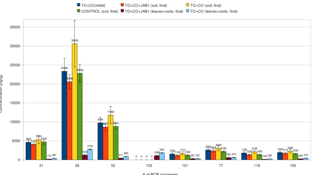
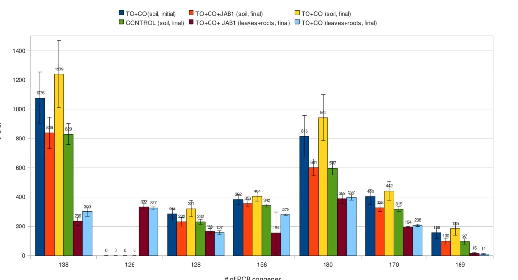
3.2 Chemical analysis
Concentration of main PCB congeners in different soil and biomass samples, measured by gas chromatografy, are shown in Table 3 to 9. Concentration of 15 main congeners [ng/g of soil or biomass] Number of main congeners Sample 31 28 52 153 101 77 118 105 138 126 128 156 180 170 169 TO + C O (s oi l; in iti al ) 3954,89 18230,60 7620,72 0,00 1101,13 2016,76 1313,16 1478,93 800,16 0,00 215,97 322,75 604,25 329,09 82,80 3957,81 18589,77 7643,43 0,00 1156,52 2035,97 1320,91 1532,44 835,55 0,00 218,09 336,74 630,29 331,56 97,58 3958,16 19006,53 7802,14 0,00 1160,66 2066,42 1352,01 1537,38 845,21 0,00 226,10 336,78 642,91 338,16 97,70 4091,98 19313,75 8087,68 0,00 1208,78 2093,88 1395,72 1560,69 867,75 0,00 230,22 342,26 647,30 338,54 109,42 4156,21 19435,44 8262,34 0,00 1237,66 2104,80 1426,16 1616,04 880,16 0,00 234,57 347,98 652,27 341,88 109,77 4201,79 20098,73 8349,34 0,00 1240,74 2160,79 1460,65 1622,67 897,60 0,00 238,24 348,99 664,06 345,14 112,89 4211,75 20164,05 8366,84 0,00 1248,94 2175,04 1468,97 1654,61 899,88 0,00 239,60 349,73 665,54 345,18 112,90 4250,30 20485,05 8444,08 0,00 1254,47 2213,45 1474,33 1665,76 909,29 0,00 240,67 350,86 668,68 349,50 113,89 4294,64 20676,31 8649,66 0,00 1265,15 2252,74 1478,04 1665,80 911,24 0,00 242,91 351,76 669,08 352,68 116,73 4334,54 20725,78 8658,23 0,00 1267,51 2260,90 1493,11 1674,91 924,77 0,00 252,89 351,81 673,90 353,38 124,04 4344,51 20728,91 8687,80 0,00 1268,53 2263,13 1510,29 1692,11 928,45 0,00 253,66 352,38 680,80 353,69 124,99 4393,19 20793,55 8713,25 0,00 1290,72 2287,16 1511,26 1702,32 931,25 0,00 256,51 355,17 687,64 355,94 126,15 4405,78 20968,49 8733,73 0,00 1298,84 2294,15 1516,73 1703,25 935,74 0,00 258,46 356,99 689,19 356,90 131,99 4432,02 21177,11 8747,22 0,00 1310,12 2294,34 1545,90 1713,30 942,21 0,00 260,36 359,29 694,45 360,36 132,49 4442,38 21240,49 8781,16 0,00 1312,69 2301,94 1558,45 1727,49 944,26 0,00 264,66 360,10 695,28 368,09 133,90 4457,93 21604,15 8886,25 0,00 1316,73 2302,52 1568,13 1730,21 951,79 0,00 265,11 370,20 715,85 378,76 139,05 4514,31 21960,84 9093,60 0,00 1375,43 2328,53 1569,14 1755,49 960,63 0,00 273,01 371,21 740,19 379,02 139,18 4526,28 22005,63 9102,97 0,00 1398,40 2332,79 1575,21 1763,97 961,73 0,00 273,18 373,83 748,60 379,63 140,64 4595,34 22066,10 9273,69 0,00 1412,29 2406,18 1576,65 1789,09 981,78 0,00 275,20 374,80 753,52 382,94 143,70 4602,49 22563,41 9277,67 0,00 1419,64 2429,38 1616,77 1803,61 994,94 0,00 280,44 375,95 770,86 383,85 147,50 Table 3: Concentration of 15 main congeners in vegetated soil samples; TO+CO(soil; initial)=contaminated soil vegetated with tobacco at the beginning of the experiment; continues in table 4.Concentration of 15 main congeners [ng/g of soil or biomass] Number of main congeners Sample 31 28 52 153 101 77 118 105 138 126 128 156 180 170 169 TO + C O + JA B 1 (s oi l; in iti al ) 4605,83 22862,07 9938,78 0,00 1473,82 2586,86 1918,17 1979,47 1105,79 0,00 281,64 380,55 842,15 401,70 158,36 4607,57 23951,45 10043,88 0,00 1563,51 2764,24 1945,96 2091,83 1131,13 0,00 283,84 381,07 898,83 417,09 165,92 4634,08 24208,50 10136,21 0,00 1621,98 2775,34 1965,10 2093,21 1156,64 0,00 292,03 389,00 901,72 419,93 169,07 4636,59 24272,48 10170,70 0,00 1633,84 2794,62 1969,24 2104,85 1168,15 0,00 295,69 391,22 902,55 431,59 171,93 4653,60 24407,98 10191,94 0,00 1646,82 2802,11 1988,16 2106,57 1180,32 0,00 300,48 391,81 909,72 438,37 175,99 4655,11 24441,23 10340,41 0,00 1652,93 2802,85 1989,03 2113,19 1187,63 0,00 303,05 393,15 910,86 441,01 180,67 4721,24 24442,70 10511,39 0,00 1657,37 2804,15 2042,78 2113,60 1189,33 0,00 304,29 394,24 914,09 442,13 182,15 4767,45 25259,65 10520,18 0,00 1679,19 2817,38 2080,18 2122,25 1208,20 0,00 309,34 395,71 918,94 442,78 182,31 4782,73 25406,15 10608,60 0,00 1722,80 2853,40 2085,11 2128,36 1218,90 0,00 310,54 396,00 928,10 444,22 182,67 4793,19 25589,05 10666,14 0,00 1738,04 2873,99 2092,05 2177,12 1219,39 0,00 311,41 401,30 929,41 444,27 185,60 4829,90 25653,45 10733,53 0,00 1741,82 2909,16 2096,39 2181,93 1223,26 0,00 311,46 409,24 940,77 446,00 190,73 4834,50 25738,82 10774,74 0,00 1749,43 2915,54 2098,86 2205,55 1229,72 0,00 313,51 409,75 941,38 447,10 191,22 4871,65 25758,37 10888,20 0,00 1754,13 2930,58 2105,26 2207,51 1240,19 0,00 321,18 412,54 959,31 449,91 192,24 4887,73 26053,07 10934,81 0,00 1781,09 2955,15 2131,66 2211,13 1265,84 0,00 324,64 421,48 961,81 452,97 194,98 4950,16 26368,12 11176,58 0,00 1785,51 3005,05 2132,38 2220,50 1283,22 0,00 326,33 422,39 962,55 458,85 200,33 5088,19 26490,75 11248,40 0,00 1844,06 3056,36 2133,28 2236,19 1293,96 0,00 338,34 425,04 971,06 466,42 200,75 5137,41 27495,15 11686,32 0,00 1890,56 3058,07 2170,63 2301,67 1302,40 0,00 342,19 425,73 979,23 468,49 200,97 5407,97 28954,51 12239,73 0,00 2054,15 3260,60 2187,49 2417,70 1303,76 0,00 351,51 451,76 979,30 479,56 211,40 5847,82 31906,09 13003,43 0,00 2241,07 3477,27 2417,68 2590,99 1366,58 0,00 368,39 453,61 1084,81 480,25 221,27 6071,49 33292,20 13583,95 0,00 2335,95 3614,42 2535,23 2681,24 1472,26 0,00 371,07 460,05 1094,46 512,86 245,28 average 4622,76 23359,66 9764,49 0,00 1527,83 2591,95 1795,41 1941,87 1076,28 0,00 284,02 382,38 815,64 402,74 156,03 st.dev. 450,45 3441,56 1440,38 0,00 300,20 412,67 335,41 306,93 176,96 0,00 41,02 34,21 142,12 51,60 39,26 Table 4: Concentration of 15 main congeners in augmented soil samples; TO+CO+JAB1(soil; initial)=contaminated soil vegetated with tobacco and augmented with Pseudomonas sp. JAB1 at the beginning of the experiment; st.dev.=standard deviation.
Concentration of 15 main congeners [ng/g of soil or biomass] Number of main congeners Sample 31 28 52 153 101 77 118 105 138 126 128 156 180 170 169 TO +C O +J A B 1 (s oi l; fin al ;) 3579,34 18438,95 7765,23 0,00 967,26 2090,56 1148,89 1474,92 715,23 0,00 192,33 0,00 529,41 293,74 68,27 3650,00 18657,00 7879,04 0,00 988,33 2117,33 1202,67 1499,40 744,24 0,00 197,39 333,15 533,17 294,23 75,38 3702,14 18726,43 7937,75 0,00 995,17 2140,13 1214,67 1550,30 750,00 0,00 206,68 337,57 550,11 294,24 78,31 3793,91 19107,03 8025,12 0,00 1026,35 2147,79 1218,07 1552,57 761,99 0,00 207,23 338,41 558,83 303,51 78,87 3810,99 19251,51 8031,05 0,00 1038,43 2155,93 1225,17 1558,64 770,99 0,00 215,23 340,18 571,73 310,24 90,78 3815,95 19599,26 8156,22 0,00 1047,94 2165,74 1249,65 1594,75 779,29 0,00 216,45 341,34 572,98 314,37 90,97 3883,91 19671,62 8167,26 0,00 1058,63 2181,30 1258,72 1603,41 800,92 0,00 220,14 342,26 575,67 317,14 91,60 3927,82 19692,65 8293,62 0,00 1067,91 2192,77 1271,00 1623,21 801,55 0,00 221,12 342,29 580,88 318,64 96,11 3943,20 19729,27 8317,97 0,00 1068,46 2197,47 1276,95 1627,12 802,04 0,00 224,45 344,22 581,88 320,11 96,68 3959,51 20018,71 8375,31 0,00 1078,04 2259,48 1287,49 1629,14 810,64 0,00 225,47 350,63 582,27 321,56 98,10 3967,75 20021,89 8386,87 0,00 1119,79 2280,38 1291,13 1635,63 812,77 0,00 226,19 352,31 585,36 325,61 98,28 4031,17 20091,39 8414,51 0,00 1134,98 2288,81 1292,40 1652,29 817,48 0,00 231,42 354,99 586,49 326,55 98,88 4056,46 20181,78 8498,71 0,00 1136,75 2314,82 1292,65 1654,44 820,70 0,00 235,03 355,50 597,55 330,26 102,03 4182,81 21245,22 8559,11 0,00 1142,06 2327,81 1298,23 1658,77 823,52 0,00 235,59 360,62 599,00 330,58 102,15 4305,16 21316,30 9007,45 0,00 1145,60 2375,00 1321,13 1688,58 859,91 0,00 237,94 362,51 603,48 330,99 107,05 4313,15 21629,18 9032,22 0,00 1194,11 2379,15 1331,23 1722,56 876,98 0,00 238,74 366,26 620,06 334,61 111,81 4502,46 22114,12 9183,41 0,00 1217,32 2436,14 1340,55 1758,95 885,72 0,00 252,20 371,73 629,00 357,38 114,49 4757,84 22950,75 9310,90 0,00 1273,38 2440,62 1437,34 1793,53 923,02 0,00 257,12 381,14 703,52 360,68 128,99 4809,97 23800,15 10459,67 0,00 1713,67 3281,57 1772,03 2387,92 1072,42 0,00 290,87 389,92 725,09 380,11 131,64 5094,08 25673,35 11220,68 0,00 1869,79 3511,83 1849,42 2530,50 1154,49 0,00 310,89 391,72 734,94 400,61 146,80 average 4104,38 20595,83 8651,11 0,00 1164,20 2364,23 1328,97 1709,83 839,19 0,00 232,12 355,85 601,07 328,26 100,36 st.dev. 411,39 1868,58 873,05 0,00 229,81 370,18 175,87 269,09 107,17 0,00 28,81 17,46 57,57 27,96 19,52 Table 5: Concentration of 15 main congeners in augmented soil samples; TO+CO+JAB1(soil; final)=contaminated soil vegetated with tobacco and augmented with Pseudomonas sp. JAB1 at the end of the experiment; st.dev.=standard deviation.
Concentration of 15 main congeners [ng/g of soil or biomass] Number of main congeners Sample 31 28 52 153 101 77 118 105 138 126 128 156 180 170 169 TO +C O (s oi l; fin al ) 4231,65 24394,18 9534,87 0,00 1259,63 2462,05 1771,44 1812,01 1024,41 0,00 258,44 363,09 771,19 378,35 127,58 4450,74 25207,99 9945,51 0,00 1321,73 2467,97 1778,61 1875,55 1032,32 0,00 265,04 365,92 798,67 380,61 129,32 4489,66 25700,50 10007,11 0,00 1332,55 2546,01 1800,85 1899,87 1044,20 0,00 268,52 367,56 800,15 383,16 132,38 4497,52 25758,12 10013,63 0,00 1385,30 2559,48 1803,27 1902,50 1061,92 0,00 272,50 373,24 800,90 383,72 146,90 4526,24 25812,71 10070,59 0,00 1404,38 2581,98 1812,58 1903,05 1064,97 0,00 275,86 373,33 810,31 384,52 149,83 4568,86 26312,03 10266,76 0,00 1409,20 2588,24 1815,55 1934,88 1069,09 0,00 283,39 378,63 824,26 385,37 150,96 4590,60 26832,50 10424,23 0,00 1413,66 2603,34 1819,72 1953,51 1070,25 0,00 288,42 382,06 826,27 388,00 160,58 4668,08 26842,00 10453,01 0,00 1439,12 2606,04 1861,23 1960,69 1087,60 0,00 290,56 383,17 838,14 404,32 162,82 4693,47 27378,78 10527,66 0,00 1478,34 2608,02 1864,89 1965,90 1087,68 0,00 292,76 385,01 850,80 415,61 164,43 4827,57 27452,84 10530,51 0,00 1490,70 2619,08 1867,08 1984,38 1100,30 0,00 300,21 388,20 893,18 416,52 165,02 4876,83 27518,59 10686,08 0,00 1517,89 2822,61 1986,46 2130,47 1162,22 0,00 301,94 408,39 903,45 425,14 178,24 4887,05 28311,83 10859,45 0,00 1608,73 2845,28 2030,14 2166,62 1175,01 0,00 307,96 411,47 905,66 430,27 179,28 4987,33 28888,01 11030,37 0,00 1660,49 2886,17 2041,70 2168,59 1222,78 0,00 311,65 415,10 912,80 441,56 187,65 5156,37 29876,12 11398,91 0,00 1728,92 2997,51 2071,98 2247,09 1236,01 0,00 331,77 422,15 917,31 448,17 203,76 6492,55 36387,46 13605,88 0,00 2036,14 3511,08 2398,70 2618,34 1370,46 0,00 351,80 429,33 1091,50 499,71 209,18 6631,20 37137,01 14646,76 0,00 2223,00 3762,66 2627,72 2788,47 1479,89 0,00 357,78 433,95 1130,57 504,19 227,00 6752,77 38917,09 14944,70 0,00 2245,60 3825,50 2665,99 2852,93 1551,01 0,00 403,12 439,07 1148,49 520,04 227,13 7047,58 40665,99 15101,62 0,00 2294,85 3929,15 2708,77 2922,22 1580,51 0,00 405,26 449,52 1184,16 536,46 240,18 7103,44 41134,04 15716,25 0,00 2489,33 4350,18 2912,25 3243,96 1666,12 0,00 411,71 456,10 1216,04 553,05 273,49 7355,70 42201,01 16274,69 0,00 2554,77 4404,42 2916,04 3269,47 1699,50 0,00 442,84 461,18 1227,10 568,84 279,30 average 5341,76 30636,44 11801,93 0,00 1714,72 3048,84 2127,75 2280,03 1239,31 0,00 321,08 404,32 942,55 442,38 184,75 st. dev. 1077,53 6136,05 2267,02 0,00 424,10 654,21 409,64 481,01 229,97 0,00 55,62 32,33 158,23 64,06 45,45 Table 6: Concentration of 15 main congeners in vegetated soil samples; TO+CO(soil; final)=contaminated soil vegetated with tobacco at the end of the experiment; st.dev.=standard deviation.
Concentration of 15 main congeners [ng/g of soil or biomass] Number of main congeners Sample 31 28 52 153 101 77 118 105 138 126 128 156 180 170 169 C O N TR O L (s oi l; fin al ) 3862,55 18438,78 7222,92 0,00 889,64 1802,65 1057,41 1270,70 671,07 0,00 196,73 0,00 511,59 285,23 72,26 4127,09 19632,05 7744,43 0,00 950,27 1911,70 1157,48 1362,69 735,70 0,00 207,15 323,20 539,06 296,98 72,43 4148,08 21135,95 8108,96 0,00 1091,90 1930,89 1203,80 1447,27 741,30 0,00 214,86 331,67 562,77 298,15 76,51 4333,61 21239,23 8236,85 0,00 1100,39 2020,15 1260,32 1483,07 786,00 0,00 215,96 331,96 563,57 299,28 78,42 4371,08 21318,05 8321,33 0,00 1100,52 2093,76 1270,60 1502,22 791,07 0,00 216,40 332,14 567,80 304,59 85,92 4412,15 21354,23 8345,96 0,00 1105,08 2098,11 1273,26 1516,15 795,19 0,00 219,21 332,88 568,11 305,21 87,43 4443,75 21548,99 8352,21 0,00 1116,64 2105,74 1279,36 1536,55 797,86 0,00 221,36 335,11 570,47 309,46 87,54 4512,50 21819,92 8478,71 0,00 1128,32 2146,23 1294,06 1556,16 800,89 0,00 231,56 335,36 571,18 311,00 87,63 4530,10 21912,20 8563,52 0,00 1163,32 2156,44 1319,23 1561,73 801,69 0,00 231,75 335,66 571,41 312,60 87,75 4566,54 22245,01 8610,37 0,00 1177,14 2157,25 1377,34 1589,18 805,65 0,00 231,90 339,40 572,36 315,94 92,75 4650,71 22515,46 8798,49 0,00 1185,62 2164,24 1385,13 1615,79 856,71 0,00 232,26 342,66 599,98 318,96 93,40 4675,17 22619,52 8807,04 0,00 1237,27 2207,36 1385,69 1629,60 859,51 0,00 236,88 343,06 603,03 319,87 97,26 4675,22 23348,08 9082,67 0,00 1275,18 2253,23 1388,31 1635,95 870,93 0,00 236,95 346,31 607,53 323,29 103,52 4750,07 23849,44 9224,93 0,00 1285,15 2297,22 1445,41 1696,76 883,81 0,00 238,43 349,10 611,16 323,31 107,76 4828,25 24132,01 9320,77 0,00 1339,86 2329,90 1455,00 1707,96 894,90 0,00 240,40 349,43 624,54 327,97 113,61 4955,87 24182,31 9330,36 0,00 1361,50 2357,89 1466,35 1726,85 898,48 0,00 246,58 350,99 642,43 331,28 116,63 4962,35 24908,33 9546,44 0,00 1372,45 2366,80 1471,08 1732,44 910,85 0,00 251,17 356,23 645,61 336,44 117,24 5150,62 24951,62 9884,37 0,00 1373,04 2374,85 1474,74 1735,21 925,24 0,00 252,18 359,69 660,68 342,13 119,32 6202,15 27152,96 9962,13 0,00 1376,49 2400,66 1498,55 1777,59 931,73 0,00 252,65 360,12 662,23 348,96 121,02 6487,41 28425,51 10338,03 0,00 1407,81 2463,74 1533,26 1784,42 1164,22 0,00 257,99 412,92 676,61 366,46 130,20 average 4732,26 22836,48 8814,02 0,00 1201,88 2181,94 1349,82 1593,41 829,40 0,00 231,62 342,41 596,61 318,86 97,43 st.dev. 632,35 2373,23 777,48 0,00 146,40 177,71 125,15 138,77 71,09 0,00 16,51 9,94 44,39 19,61 17,61 Table 7: Concentration of 15 main congeners in bulk soil soil samples; CONTROL(soil; final)=contaminated bulk soil at the end of the experiment.
Concentration of 15 main congeners [ng/g of soil or biomass] Number of main congeners Sample 31 28 52 153 101 77 118 105 138 126 128 156 180 170 169 TO + C O + JA B 1 (le av es + ro ot s; fi na l) 139,59 1083,23 364,69 1007,06 81,84 416,75 91,13 214,05 198,26 297,53 127,50 0,00 341,19 185,08 6,48 148,13 1085,35 365,38 1020,49 125,92 422,02 97,63 225,64 204,57 304,98 134,22 0,00 354,75 185,19 8,41 158,67 1098,85 371,90 1020,52 147,75 430,75 102,17 227,88 209,38 310,84 153,90 0,00 355,03 185,47 9,38 161,62 1111,55 377,66 1027,20 167,43 453,20 114,56 230,28 210,28 313,97 154,17 0,00 363,23 186,53 10,09 162,48 1122,71 382,17 1055,25 175,15 497,00 119,53 232,51 224,65 318,12 158,11 0,00 366,34 189,61 10,69 162,68 1155,56 394,41 1057,03 195,61 509,79 124,92 234,80 226,01 319,18 159,53 0,00 371,66 190,17 10,74 165,28 1168,96 396,21 1066,67 221,36 532,92 126,58 242,37 230,79 329,64 159,70 0,00 373,29 190,64 11,37 166,45 1186,00 396,82 1067,48 227,62 550,17 127,39 245,56 231,05 330,01 162,33 0,00 375,66 193,58 11,39 166,75 1217,66 399,40 1068,08 236,60 561,39 130,52 247,46 231,61 330,07 163,28 269,25 381,81 194,12 15,00 166,95 1220,33 405,37 1072,74 236,63 564,98 135,48 249,28 233,50 331,88 165,16 270,07 386,00 196,27 18,72 175,93 1229,61 406,88 1099,40 274,24 576,59 136,54 253,48 234,63 334,29 165,56 273,48 388,73 196,29 18,93 176,87 1275,78 419,67 1128,50 319,25 577,31 137,69 253,61 234,85 337,37 167,93 274,94 407,01 197,84 19,20 177,39 1279,05 426,41 1133,25 341,19 578,88 138,15 256,14 237,08 340,79 173,03 275,78 409,66 197,91 20,09 181,13 1282,47 427,19 1136,00 353,48 607,52 142,41 257,97 241,69 344,17 176,77 276,54 410,08 200,51 20,45 186,10 1330,48 458,26 1147,78 362,55 639,97 150,31 269,61 246,90 351,57 176,81 278,03 421,93 204,08 20,75 186,44 1337,93 503,23 1161,91 445,64 643,93 154,18 274,06 259,79 357,19 180,92 281,60 449,30 204,38 23,26 186,95 1578,02 505,15 1164,32 446,34 679,15 158,68 284,86 278,93 368,82 196,22 287,12 457,89 205,66 24,11 195,08 1602,92 512,94 1176,12 451,91 747,59 188,60 287,02 309,83 378,21 200,15 289,28 8749,00 251,61 27,02 average 170,25 1242,58 417,43 1089,43 267,25 554,99 128,43 249,26 235,77 333,26 165,29 154,23 388,53 194,24 15,89 st.dev. 14,29 150,10 47,53 55,10 113,89 90,94 18,74 20,37 26,68 21,42 18,03 142,03 31,75 6,76 6,19 Table 8: Concentration of 15 main congeners in biomass samples; TO+CO+JAB1(leaves+roots; final)=tobacco plants cultivated in contaminated soil augmented with Pseudomonas sp. JAB1, harvested at the end of the experiment.
Concentration of 15 main congeners [ng/g of soil or biomass] Number of main congeners Sample 31 28 52 153 101 77 118 105 138 126 128 156 180 170 169 TO + C O (l ea ve s + ro ot s; fi na l) 345,79 2561,10 765,28 1714,24 247,03 472,60 222,34 355,89 236,09 307,00 137,66 0,00 362,84 197,04 5,32 350,10 2594,31 811,22 1735,49 251,93 507,60 227,13 386,33 271,18 309,52 140,11 273,27 371,32 197,50 5,88 367,16 2615,29 816,83 1762,01 252,45 526,11 231,47 388,36 275,17 310,34 140,49 273,29 378,97 197,57 6,14 368,78 2656,07 828,60 1770,88 253,99 563,86 233,41 391,42 280,84 314,38 141,13 274,51 379,39 198,24 7,00 377,55 2675,98 836,13 1782,16 256,09 578,88 243,11 394,07 281,11 316,55 148,64 274,51 385,67 201,08 7,12 378,83 2683,36 839,81 1784,11 258,64 584,85 243,70 398,15 282,17 318,44 154,82 276,61 388,94 205,82 8,16 379,17 2706,60 845,18 1787,06 271,42 591,64 244,60 402,01 285,94 319,77 157,89 277,81 390,31 206,10 8,48 383,00 2722,38 846,27 1801,21 278,37 610,09 245,45 414,66 286,07 323,18 158,27 278,43 391,73 206,62 9,69 388,67 2730,52 848,49 1804,56 278,49 614,67 251,51 420,04 289,29 328,06 159,74 279,00 393,09 209,14 10,74 388,93 2734,02 858,54 1818,92 281,23 641,05 253,41 424,36 293,42 330,52 160,77 279,37 398,92 209,50 11,61 392,47 2758,50 862,11 1855,65 285,60 643,68 254,36 424,74 305,62 330,72 161,35 279,50 399,05 210,05 12,44 393,03 2771,06 880,99 1856,46 288,53 645,38 258,60 434,58 310,41 331,66 162,35 279,59 403,62 210,62 12,52 395,41 2817,47 883,55 1865,40 295,06 648,47 259,96 435,63 315,76 333,87 162,37 280,45 407,52 213,41 12,89 400,05 2840,76 902,28 1868,63 314,63 648,49 261,63 442,24 317,23 333,87 162,37 280,53 411,08 213,52 13,43 406,64 2871,86 921,66 1868,88 328,90 667,18 265,50 444,30 320,21 335,55 163,40 281,48 413,41 214,37 15,04 408,24 2889,13 922,32 1875,47 344,48 685,02 274,06 444,86 322,36 341,80 163,88 283,78 415,96 215,82 15,16 416,65 2924,02 937,82 1890,11 354,34 710,38 278,69 451,85 355,31 345,43 165,34 286,14 420,70 217,25 16,05 416,66 2942,31 970,64 1941,05 391,57 716,26 283,43 481,76 375,36 350,64 186,04 287,78 431,47 221,45 21,36 average 386,51 2749,71 865,43 1821,24 290,71 614,24 251,80 418,63 300,20 326,74 157,03 279,18 396,89 208,06 11,06 st.dev. 20,18 112,43 50,85 59,67 40,88 67,19 17,30 30,25 32,04 12,66 11,85 4,15 17,96 7,41 4,27 Table 9: Concentration of 15 main congeners in biomass samples; TO+CO(leaves+roots; final)=tobacco plants cultivated in contaminated soil, harvested at the end of the experiment. Previous data were processed with ANOVA Test (ANalysis Of VAriance Test; Table 11, 12) to highlight differences between soil combinations and biomass samples. Averages and standard deviation were calculated to have unambiguous results (Table 10). TO+CO(soil, initial) and TO+CO+JAB1(soil, initial) measurements were put together to represent situation in vegetated soil at the beginning of the experiment; they were labelled as TO+CO(soil, initial).