Universit`
a degli Studi di Pisa
FACOLT `A DI SCIENZE MATEMATICHE FISICHE E NATURALI
Corso di Laurea Specialistica in Geofisica di Esplorazione ed Applicata
Tesi di Laurea Specialistica
Earthquake-induced rotational ground motions
from G-Pisa ring laser gyroscope
Candidato:
Andrea Licciardi
Matricola 459514
Relatore:
Prof. Gilberto Saccorotti
Correlatore:
Dr. Jacopo Belfi
Controrelatore:
Contents
1 Introduction and aim 1
2 Basic theory 5
2.1 Introduction . . . 5
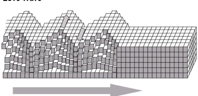
2.2 Love-waves . . . 7
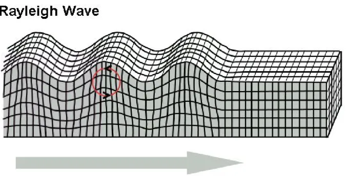
2.3 Rayleigh-waves . . . 8
2.4 Applications . . . 11
3 Instrumentation and data 13 3.1 Gyrolaser . . . 13 3.2 Guralp seismometer . . . 19 3.3 EpiSensors . . . 21 3.4 Data . . . 22 4 Methods 23 4.1 Preprocessing . . . 23
4.2 Power Spectral Densities and MulTitaper Method . . . 24
4.3 Spectrograms . . . 25
4.4 Correlation of traces . . . 26
4.5 Azimuth estimation (Love-waves) . . . 26
4.6 Array analysis . . . 28
4.6.1 Plane Wave Fit . . . 28
4.6.2 Array-derived rotation rate . . . 30
Contents Contents
4.8 Phase velocity from collocated measurements . . . 32
4.8.1 Time domain . . . 32
4.8.2 Frequency domain . . . 34
5 Results 35 5.1 Introduction . . . 35
5.2 Love-waves . . . 35
5.2.1 Azimuth and phase velocity determination . . . 38
5.3 Rayleigh-waves . . . 43
5.3.1 Japan earthquake . . . 43
5.3.2 Regional earthquakes . . . 61
6 Conclusions 65
Chapter 1
Introduction and aim
Seismologists have measured for decades the translational components of ground motion due to different kind of sources (both natural and artificial). These components are usually referred as N (north-south) E (east-west) and Z (vertical) or R (radial), T(tangential) and Z(vertical). A complete representation of ground motion induced by earthquakes needs not only these three translational components but also six components of strain and three components of rotational motion (Aki and Richards, 2002). The latter has always been very difficult to measure, because of the small amplitudes even in the vicinity of the source. Various attempts to measure rotational motion induced by earthquakes have been made in the history of seismology. Pioneering studies in this sense are those carried out by Cecchi(1876) and Galitzin (1912), who proposed different ways to perform such measurements. Despite these first attempts, the widespread belief that rotational motions were insignificant had continued for many years later. For example Richter himself 1958 in one of his footnotes wrote: “Theory indicates, and observation confirms, that such rotations are negligible”. But at that time, as we said, there were no instrument sensitive enough to measure rotational motions with a resolution better than few microradians per second. More recently, using an azimuthal array of seismographs, Droste and Teisseyre (1976) derived rotational seismograms of rock bursts from a nearby mine. Nigbor (1994) studied rotational effects recorded in the near-field of explosions using a triaxial translational accelerometer and a solid-state rotational velocity sensor. The same sensor has been used byTakeo (1998) for recording an earthquake swarm on Izu peninsula, Japan. However,
1 Introduction and aim
because of the limitation of the instrument sensitivity, this kind of sensor was only able to sense the rotational ground motion near the earthquake sources or other artificial sources. This explains why Aki and Richards (2002) stated “...as of this writing seismology still awaits a suitable instrument for making such measurements”.
In the last years, thanks to the development of laser technology, a new kind of instrument began to be available. Ring-laser gyroscopes, working on Sagnac effect are providing an interesting tool to investigate rotational ground motion (Schreiber,2006; Stedman, 1997). Several observations have been made with this instruments, starting from Stedman et al.
(1995), McLeod et al. (2009) and Pancha et al. (2000) that have reported a sufficient sensor sensitivity to record rotational motion for seismology. Rotational motion induced by earthquakes has been measured intensively with the ring-laser gyroscope installed at the fundamental station Wettzell, Germany (Cochard et al., 2006; Gebauer et al., 2012;Igel et al., 2005, 2007). These authors showed the great correlation between gyrolaser (rotational motion) and collocated seismic sensor (translational motion) recordings, both in amplitude and in phase, as predicted by theory. Phase velocity and direction of propagation of the seismic wavefield have also been investigated (Gaebler,2010; Igel et al., 2005,2007;Kurrle et al., 2010; Suryanto, 2006) using collocated measurement of rotation and translation. Another way to estimate rotations have been proposed by some authors using array of seismic sensors (Bodin, 1997; Huang, 2003; Spudich and Fletcher, 2008; Spudich et al.,
1995), comparisons between this kind of estimations and direct measurement of rotation from Wettzell gyrolaser has also been carried out by Suryanto et al. (2006) and have shown good agreement, but with important limitations due to the assumptions behind the array-derived rotation rate method.
This thesis focuses on the data collected by the G-Pisa ring-laser gyroscope, developed by the University of Pisa (Department of Physics) and INFN (Belfi et al., 2011, 2012b;
Di Virgilio et al., 2010). This instrument has been operating for almost 2 years at the European Gravitational Observatory in Cascina (Pisa), in the framework of the VIRGO project. In particular, I report the very first seismic analysis of the rotational data from a gyrolaser lying in the vertical plane, which is sensitive to rotation about a horizontal axis (tilt). The main part of the thesis is dedicated to the analysis of the Mw=9.0, March 11th, 2011, Japan earthquake; in addition, I also account for recordings from some events
1 Introduction and aim
occurred at regional distances.
The first objective of this work is to characterize the performance of G-Pisa in relation to a collocated accelerometer and to verify the ground-coupling of the instrument. By calculating the power spectral density (PSD) of rotation rate and acceleration I first identify the signal to noise ratio as a function of frequency and, by computing time-frequency transforms (spectrograms), I individuate the most energetic frequency bands as a function of time for both the instruments during several selected earthquakes. Then, rotation rates and accelerations are correlated within subsequent frequency bands, in order to quantify similarity between the signals. The second objective of the thesis is to compare the recorded rotation rates with those obtained through an array-based analysis. Applying the seismo-geodetic method by Spudich et al. (1995), I derive the rotation rate from a tripartite array of three-components accelerometers. This method provides an independent estimation of ground rotations that should be in agreement with that directly recorded by the gyrolaser. Results from this analysis show that the two measurements are in general agreement; I attribute the discrepancies to both the geometrical setting of the array and the band limitations of its sensors. The third objective concerns phase velocities estimation and derivation of surface waves dispersion curves from collocated measurements of rotation and translation. Following Igel et al. (2005, 2007) andKurrle et al. (2010), I address this issue by calculating the zero-lag correlation coefficient between translational and rotational traces. When the correlation coefficient is above an arbitrary threshold, phase velocity is obtained through a linear regression within overlapping sliding time windows. Iterating the procedure after a narrow band-pass filtering of both traces, it is possible to derive a dispersion curve for the selected wave packet. A theoretically equivalent dispersion curve could be derived in frequency domain as shown bySuryanto (2006), both for Love-and Rayleigh-waves, simply by calculating the spectral ratios between translation Love-and rotation. I implemented this second procedure using a multitaper method (MTM,Thomson
(1982)), in order to reduce variance and bias by averaging periodograms obtained using a properly-designed taper. The dispersion curves calculated in this manner are compared to those obtained with a multi-frequency Plane Wave Fit (PWF) analysis (Del Pezzo and Giudicepietro, 2002). This method, that consists in estimating wavefield slowness for an array of sensors, provides independent information about velocities and direction
1 Introduction and aim
of propagation (azimuth) for plane waves crossing the array. Rayleigh-waves dispersion curves derived from the Japan earthquake, are then compared against the theoretical phase velocities derived from a standard (AK135) Earth Model (Kennett et al., 1995). Since Rayleigh-waves are fully recorded by the gyrolaser only when their direction of propagation is perpendicular to G-Pisa area vector, I implemented a rotation rate signal correction method that takes into account the different directions of propagation of Rayleigh-waves (as estimated from PWF inversion) with respect to G-Pisa axis of sensitivity. This correction leads to a more reliable result in estimating phase velocities, that otherwise would be overestimated. Collocated measurements of rotation about vertical axis and transverse acceleration for horizontally-polarized seismic waves (SH- and Love-waves) allow estimating direction of propagation and azimuth of the incoming wavefield. FollowingIgel et al.(2007) andHadziioannou et al. (2012) I conducted these estimates for Love waves recorded when G-Pisa was configured with the area vector oriented vertically.
This thesis is organised into five chapters. In the first chapter, I briefly report the general theory behind rotational motions, and present the relationships between rotation and translation in the context of classical elasticity. Here I show that surface-waves phase velocities and thus dispersion curves can be obtained from collocated measurements or rotation and translation. In the second chapter I present the instrumentation and data, with particular reference to G-Pisa and its ability to investigate both Rayleigh-and Love-waves with a sensitivity on the order of a few nrad/s/√Hz over the 0.02-1 Hz frequency band. In the third chapter I describe the data analysis methods, and their practical implementation in terms of Matlab scripts. In the fourth chapter I present and critically comment the results from the analysis. This chapter is divided into two sections, dedicated respectively to the Love- and Rayleigh-waves results. The last chapter is dedicated to the general discussion and conclusions.
Chapter 2
Basic theory
2.1
Introduction
Here I briefly describe the background theory of seismic rotations. All the discussion is based on classical elasticity for which the stress and strain tensors are symmetric. As pointed out byLee et al. (2009) near field observations report rotational motions which are from 10 to 100 times larger than what expected from classical elasticity theory. Theoretical work suggests that in granular materials or cracked continua asymmetries of the stress and strain tensors can create rotations separate from those predicted by classical elastodynamic theory (Pujol, 2009; Teisseyre, 2009, 2012; Teisseyre et al., 2006).
In the framework of classical elasticity and assuming infinitesimal deformations, fol-lowing Cochard et al. (2006) the displacement of a point at x is related to that of a neighbouring point x + δx by (Aki and Richards,2002):
u(x + δx) = u(x) + Gδx = u(x) + εδx + Θδx = u(x) + εδx + θ×δx
(2.1)
2 Basic theory 2.1 Introduction and θ= θx θy θz = 1 2∇×u(x) = ∂uz ∂y − ∂uy ∂z ∂ux ∂z − ∂uz ∂x ∂uy ∂x − ∂ux ∂y (2.2)
is a (pseudo-) vector which does not enter Hooke’s law and represents the angle of rigid rotation generated by the disturbance. This illustrates that one needs three components of translation, six components of strain and three components of rotation to fully characterize the change in the medium around point x.
Starting from Hooke’s Law
σij = λδij 3
X
k=1
εkk+ 2µεij (2.3)
where σij and εij are generic component of the stress and strain tensors respectively,
P3 k=1εkk= ∂ux ∂x + ∂uy ∂y + ∂uz
∂z = ∇u, λ, µ are the Lam`e constants and δij is the Kronecker delta that assumes value 1 when i = j and 0 otherwise. If we consider the free surface lying on the xy plane and under the zero traction boundary condition (e.g. σiz = 0 (i = x, y, z)),
direct application of Eq.2.3 in a homogeneous, isotropic medium leads to ∂ux ∂z = − ∂uz ∂x ∂uy ∂z = − ∂uz ∂y ∂uz ∂z = − λ λ+ 2µ( ∂ux ∂x + ∂uy ∂y ) (2.4)
2 Basic theory 2.2 Love-waves
and from2.2 we get:
θx = ∂uz ∂y θy = − ∂uz ∂x θz = 1 2( ∂uy ∂x − ∂ux ∂y ) (2.5)
The above equations give us the expression for rotation angles with respect to displacement gradient elements, under the assumptions of plane wave propagation, and zero traction boundary condition, in the next sections we are going to look at the relationship between these angles and translational components of motion for the two main types of surface waves, Love and Rayleigh-waves, to derive simple formulas that link rotation and transla-tion. We will see that in both cases, these two quantities are scaled by phase velocity, and that in principle, one can extract it by collocated measurement of rotation and translation.
2.2
Love-waves
Love-waves are horizontally polarized surface waves generated by interaction of SH-waves with the free surface (Fig. 2.1).
Being transversely polarized, the displacement for a wave propagating along X-axis can be expressed by
u(x, y, z, t) = (0, uy(t − x/CL), 0) (2.6)
with CL being horizontal phase velocity. Love-waves induce rotations about Z-axis
that using 2.2 can be expressed by θz = 1 2 ∂˙uy ∂x = − ˙ uy(t − x/CL) 2CL (2.7)
2 Basic theory 2.3 Rayleigh-waves
Figure 2.1: The particle motion of Love-waves
and for rotation rate
Ωz = ∂θz ∂t = − ¨ uy(t − x/CL) 2CL (2.8)
this means that transverse acceleration and rotation rate about Z-axis are in phase and
scaled by a factor − 1
2CL
. A ring-laser set in horizontal configuration is sensitive, in principle, only to rotation about vertical axis, that means, only to Love and SH waves that are horizontally polarized.
2.3
Rayleigh-waves
Rayleigh-waves are effectively surface waves characterized by a retrograde elliptic motion confined in the vertical plane containing the direction of propagation (Fig. 2.2). Rayleigh-waves can therefore be recorded both by the vertical component and by the horizontal
2 Basic theory 2.3 Rayleigh-waves
component of a seismic sensor.
Figure 2.2: The particle motion of Rayleigh-waves
For a simple half-space Poisson solid, the Rayleigh-waves displacements propagating along X-axis at zero depth are given by Lay and Wallace (1995) as:
ux = −αAk sin(ωt − kx)
uz = βAk cos(ωt − kx)
(2.9)
where A is the P-wave amplitude, ω is the angular frequency, x is distance, k is the Rayleigh wavenumber and α = 0.42 and β = 0.62 are constants for the Poisson solid. FollowingLin et al.(2011) we refer to X and Z directions as radial and vertical. In addition, Z direction is positive down. The velocity and acceleration of the particle motions along the X-axis and Z-axis are then:
2 Basic theory 2.3 Rayleigh-waves
Velocity (
˙ux = −αAkω cos(ωt − kx)
˙uz = −βAkω sin(ωt − kx)
Acceleration ( ¨ ux= αAkω2sin(ωt − kx) ¨ uz = −βAkω2cos(ωt − kx) (2.10)
Using2.5,we can obtain the rotation angle around Y-axis for Rayleigh-waves:
θy = −βAk2sin(ωt − kx) (2.11)
and differentiating with respect to time we get rotation rate as:
Ωy = ˙θy = −βAk2ωcos(ωt − kx) (2.12)
If we now look at the relationship between translations along X-axis ( ˙ux,u¨x) and
rotations about Y-axis (θy,Ωy)
¨ ux Ωy = −α β ω k sin(ωt − kx) cos(ωt − kx) (2.13) ¨ ux θy = −α β ω2 k = − α βCRω (2.14) ˙ ux Ωy = α β 1 k (2.15)
We can see from 2.13 that X-axis acceleration and Y-axis rotation rate are phase shifted by 90° and scaled by the phase velocity, 2.14shows that X-axis acceleration and Y-axis rotation angle are in phase and scaled by phase velocity multiplied by frequency.
2 Basic theory 2.4 Applications
Equation2.15tells us that X-axis velocity and Y-axis rotation rate are in phase and scaled by the inverse of wavenumber.
Instead by comparing translation along Z-axis and rotation about Y-axis
¨ uz
Ωy
= ω
k = CR (2.16)
we can observe that the two quantities are in phase and amplitude are scaled by a factor CR that is Rayleigh-waves phase velocity.
2.4
Applications
In the previous sections we showed that collocated measurements of rotation and translation can provide additional information about seismic wavefield. Here we briefly discuss some possible application of this method. First of all, the possibility of examining seismic wave phase velocities, as described by Igel et al. (2005,2007) and Suryanto (2006) from collocated measurements, remains one of the most interesting application that could allow to derive surface waves dispersion curve (Kurrle et al., 2010) without relying on multichannel analysis. This possibility is examined more in deep in this thesis both for Love and Rayleigh-waves. Furthermore, exploiting the phase relationship between transverse acceleration and rotation rate about the vertical axis it is possible to use collocated measurements to estimate directions of propagation of Love-waves (Gaebler,
2010; Hadziioannou et al., 2012), that until today is indirectly estimated with array techniques. Another possible fields of application regards earthquake engineering where rotational (or torsional) motions play an important role, especially in connection with the building response and in the calculation of site effects (Ghayamghamian and Matosaka,
2003). Historical examples of rotation of buildings (Fig. 2.3) are well summarized inKoz´ak
(2009) and Sargeant and Musson (2009) and used in order to develop numerical models of earthquake rotated object byHinzen (2012). Here we just recall these works for a deeper discussion on this matter.
2 Basic theory 2.4 Applications
Figure 2.3: Rotation of obelisk segments from the 1897 Assam earthquake (Oldham,1899).
Legrand (2003) showing that the representation of a finite source in the earthquake source modelling is more informative by including the rotational part that may derived from rotational motions. He also mentioned that the description of the finite source via seismic moment tensor is neglecting the rotational part that actually must be taking into account. Lastly, Bernauer et al. (2009) introduced a new technique to seismic tomography of incorporating rotational motions into the seismic inverse problems with the goal to resolve better and more realistic tomographic images.
All this possible applications require as said, an high sensitive rotational sensor that should be capable to detect rotations in a large frequencies and amplitudes range. In the next chapter we briefly describe ring-laser gyroscopes, that over the last few years are representing the most suitable instrument to achieve this task.
Chapter 3
Instrumentation and data
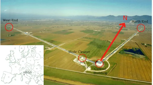
This chapter describes the instrumentation used for the experiments and the features of the collected data. To perform collocated measurements of rotation and translation the distance between the two different type of sensors must be considered small with respect to the analyzed wavelengths. This has been achieved comparing data from G-Pisa ring-laser gyroscope with seismic sensors already present at the VIRGO site (Fig. 3.1).
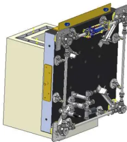
When possible, data from a Guralp CMG40-T broadband seismometer were used because of the high sensitivity of the instrument. Otherwise we used signals recorded by a triaxial EpiSensor ES-T, force balance accelerometer located at VIRGO’s central building, some 10 m apart from the ring-laser apparatus. This accelerometer, together with other two identical instruments located at the VIRGO North-end and West-end, has been used also to collect data for array analysis. The array set up is shown in Fig. 3.2. In this work, all the instruments recording ground translation have one of the sensitivity axes oriented along VIRGO’s arms thus the N-S components of translation are misaligned with respect to the geographical N of an angle of about 19° measured clockwise.
3.1
Gyrolaser
In this thesis a ring-laser gyroscope was used so the main attention is pointed to this kind of instrument. A complete description of other types of rotational sensors and their possible applications in the field of seismology can be found in literature (Bernauer et al.,
3 Instrumentation and data 3.1 Gyrolaser
Figure 3.1: Location of the VIRGO gravitational wave antenna, Cascina (Pisa). The ring-laser gyroscope G-Pisa, a Guralp CMG40-T broadband seismometer and a tri-axial EpiSensor ES-T accelerometers are located in VIRGO’s central building. VIRGO’s North arm has an azimuth of 19° with respect to the geographical North.
2012; Graizer, 2009; Jaroszewicz et al., 2011; Knejzl´ık et al., 2012; Velikoseltsev et al.,
2012) and goes beyond the scope of this work.
The rotation rates thus far observed in seismology range from 10−1 rad/s (Nigbor,
1994) close to seismic sources to 10−11rad/s for large earthquakes at teleseismic distances
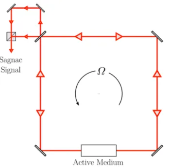
(Igel et al.,2005, 2007). Ring laser gyroscopes represents powerful tools to measure small amplitude rotations induced by earthquakes because of their insensitivity to transla-tional and cross-rotatransla-tional motions. Ring lasers detect the Sagnac beat frequency of two counter-propagating laser beams (Stedman, 1997) as sketched in Fig3.3. These active interferometers are composed by triangular or square optical cavities under vacuum in which the light beams interfere. If the reference frame of the instrument rotates, the effective cavity length between the co-rotating and the counter-rotating lightbeams differs, and the two beams are frequency split. Such frequency splitting is then measured as the
3 Instrumentation and data 3.1 Gyrolaser
Figure 3.2: Array setup. EpiSensor accelerometers used for the array experiments are indicated by blue arrows.
beat frequency of the two beams outside the cavity. This beat frequency (Sagnac frequency fS) is related to the rotation rate by a scale factor. For a ring-laser with perimeter P ,
area vector A = Aˆn, and laser wavelength λ, the angular velocity Ω of its reference frame induces a Sagnac frequency given by:
fS =
4A
P λ Ω · ˆn (3.1)
fS depends on the geometrical scale factor
4A
P λ, on ˆn (changing in orientation of the instrument) and finally on Ω (due to changes in Earth’s rotation rate, or seismically induced rotations) that represents the most dominant contributions to fS. In seismic
application the Earth’s rotation rate plays the role of a constant bias for the sensor. On the other hand, very sensitive ring-laser are able to detect Earth rotation rate variations such as the one induced by polar motion or the free oscillation of the Earth rotation axis known as Chandler Wobble (Igel et al.,2011;Schreiber et al., 2004, 2011).
G-Pisa is a He-Ne based gyrolaser with λ = 632.8nm. It operates in a squared cavity with A = 1.82m2 (Belfi et al.,2010,2011;Di Virgilio et al.,2010). The instrument has been
3 Instrumentation and data 3.1 Gyrolaser
Figure 3.3: Ring laser gyroscope diagram. Ω leads the ring-laser to rotate with respect to an inertial frame, the cavity length for the two counter-propagating laser beams becomes different and one observes a beat frequency (Sagnac frequency).
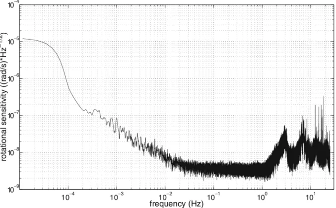
working since July 2010 at the VIRGO site (latitude φ= 43°37’53”, and expected mean value for the Sagnac frequency due to the Earth rotation bias of about 106.2 Hz) with a sensitivity of some (nrad/s)/√Hz in the range 10 − 100 mHz as reported by Di Virgilio et al.(2010) and Belfi et al. (2012b) and shown in Fig. 3.4.
The beat frequency between the two counter-propagating gyrolaser beams is detected by a photodetector and acquired by the VIRGO data acquisition system at the rate of 5 kHz. The rotation rate signal is then reconstructed up to the frequency of 50 Hz by using the following procedure:
• The optical beat signal v(t) is bandpass- filtered (with a digital first-order Chebyshev filter) around the nominal Sagnac frequency within a bandwidth of about 90 Hz.
• The filtered signal and its Hilbert transform w(t) are combined to form the analytic signal z(t) = v(t) + jw(t).
• By expressing the analytic signal in the form z(t) = |z(t)|exp[jφ(t)] , the instanta-neous phase is estimated as φ(t) = 2πfSt
3 Instrumentation and data 3.1 Gyrolaser
Figure 3.4: (Belfi et al., 2012b). Typical angular velocity sensitivity of the gyroscope operating in the vertical plane configuration
• The instantaneous frequency fS , connected to the rotation rate by the Eq.3.1, is
finally estimated by calculating the derivative of the unwrapped instantaneous phase φ.
• The instantaneous frequency is down-sampled down to the final sampling frequency of 50 Hz and converted to rad/s.
The possibility of changing G-Pisa configuration between horizontal and vertical allows to study rotations, around vertical and horizontal axis (Fig. 3.5). From a seismological point of view this means that assuming plane polarized waves propagation, it is possible to measure rotation induced by different kind of seismic waves. When G-Pisa is placed in horizontal configuration is sensitive to rotation about Z-axis that are induced by horizontally polarized waves (SH- and Love-waves). On the other hand a vertical configuration of G-Pisa allows to measure rotation about one of the two horizontal axis (e.g. X-axis)
3 Instrumentation and data 3.1 Gyrolaser
induced by waves propagating along and transversely polarized on the vertical plane (Y-Z plane). These are (a) P-wave, as a consequence of wave reflection–conversion at the free surface, (b) SV-waves, and (c) Rayleigh-waves. In this thesis data from both types of configurations have been analyzed and major attention has been given to surface waves (Love and Rayleigh-waves), exploiting the relationships between translation and rotation
discussed in chapter 2.
Figure 3.5: The two possible G-Pisa configurations. On the left, horizontal configuration is sensitive to rotation about Z-axis. On the right, vertical configuration records rotation about an horizontal axis.
3 Instrumentation and data 3.2 Guralp seismometer
3.2
Guralp seismometer
For the acquisition of the translational ground motions a three-component Guralp CMG40-T broadband seismometer was used (Fig. 3.6). The seismometer, already present at the
Figure 3.6: Guralp CMG40-T broadband seismometer
VIRGO site, is located at a distance less than 10 m from the ring-laser and in the same building, so the two instruments are considered collocated with respect to the analyzed frequency range (from 0.005 to 5Hz) which implies wavelengths spanning the 105− 102
m range. Mechanically, the vertical and horizontal sensor constructions are very similar. The vertical component sensor boom is supported horizontally with a leaf spring. The horizontal sensor is based on an inverted pendulum which is supported with two parallel leaf springs. The vertical and horizontal sensors are orthogonal to each other. The three sensors are controlled by a force feedback system to give velocity and mass position electrical outputs. The relative motion of the mass to the frame is detected by a differential capacitor which provides the basic signal from the device. The basic response of the system (velocity output) is flat to velocity from a specified corner frequency of fn to 50 Hz (f is
3 Instrumentation and data 3.2 Guralp seismometer
the long period corner frequency). The damping coefficient of the sensor transfer function is η = 0.707. Here is a table of specifications
FLAT-RESPONSE (VELOCITY) 30s – 50 Hz
SENSITIVITY 800 V/m/s
DIFFERENTIAL OUTPUT ±10 V
3 Instrumentation and data 3.3 EpiSensors
3.3
EpiSensors
Unfortunately, as in the case of the MW=9.0, March 11th, Japan earthquake, it happened
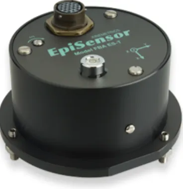
that some records coming from the Guralp CMG40-T broadband seismometer were not usable, indeed, because of VIRGO’s experiments necessity, it was operating with a high gain level in order to monitor the microseismic activity with high sensitivity, and thus, earthquakes signals resulted severely clipped. In this cases, translational measurements have been carried out with an EpiSensor FBA ES-T Kinemetrics force balance accelerometer (Fig. 3.7). An array of three of these accelerometers has also been used as discussed in the
introduction (Fig. 3.2).
The EpiSensor is a triaxial accelerometer optimized for earthquake recording applications.
Figure 3.7: EpiSensor FBA ES-T force balance accelerometer
Inside the waterproof, anodized-aluminum housing are three orthogonally mounted low-noise EpiSensor force balance accelerometer modules.
DYNAMIC RANGE 155 dB + (EpiSensor noise model
available from Kinemetrics)
BANDWIDTH DC to 200 Hz
FULL-SCALE OUTPUT User-selectable at: ±2.5V single-ended;
±10V single-ended; ±5V , ±20V differential
3 Instrumentation and data 3.4 Data
3.4
Data
Table3.3 reports reports a list of the analyzed earthquakes. For each event is specified the G-Pisa configuration and the translational sensor used.
DATE TIME LAT LONG Mω LOCATION G-Pisa TRANSL.
(UTC) (deg) (deg) (deg) SENSOR
2010-Oct-13 22:43:14 44.14 12.37 4.1 Rimini horiz. Gur.
2010-Nov-03 00:55:42 43.76 20.73 5.5 Serbia horiz. Gur.
2010-Nov-03 18:13:05 40.00 13.16 4.9 Tyrrhenian horiz. Gur.
2011-Mar-11 05:46:24 38.29 142.373 9.0 Japan vert. EpiS.
2011-Jul-07 19:21:48 42.03 7.72 5.3 Tyrrhenian vert. EpiS.
2011-Jul-17 18:30:28 45.00 11.29 4.9 Po plain vert. EpiS.
2010-Jul-25 12:31:20 44.98 7.284 4.4 Hautes- vert. EpiS.
Alpes
Table 3.3: Parameters of the observed events. G-Pisa configuration and the type of translational sensor used are reported for each event in the last two columns.
Chapter 4
Methods
This chapter summarizes the processing methods used through the whole data analysis. As most of the work is based on data collected by G-Pisa in vertical configuration, methods must be considered valid only for this kind of analysis, I will explicitly mention when the methods were used both for Love and Rayleigh-waves analysis or only for Love-waves (G-Pisa in horizontal configuration). For the whole data processing MATLAB software was used. For each of the next sections it will be given a brief review of the the theory behind each method used and a description of how it has been implemented. Results obtained with the described methods will be presented and commented in the next chapter.
4.1
Preprocessing
Data coming from G-Pisa comes in unit of rad/s, that means rotation rate. EpiSensors measure acceleration and so are in unit of m/s2, while data from seismometer are velocity
expressed in m/s. When it was necessary signals have been integrated or differentiated to obtain the desired output. It will be told in the next sections when these operation have been carried out. This preprocessing section will describe the basic operations that have preceded the analysis of the data. First, for each seismic event, traces were cut to isolate earthquakes starting from origin time up to an adequate ending time. The selected portion of the record has been demeaned, simply by removing the mean value from the
4 Methods 4.2 Power Spectral Densities and MulTitaper Method
entire portion, detrended, to remove linear trend affecting the record, and tapered with a Tukey window of the same length of the analyzed portion. For each event a different linear range of periods has been chosen according to the frequency content. A narrow-bandpass filtering around the selected periods has been done, to investigate the properties of traces in frequency domain. Filtering has always been performed with a 4th order Butterworth bandpass filter, chosen for its flat response in the passband. The filter was applied forward and backward to avoid a phase shift in the resulting filter trace. In the case of the aforementioned narrow-band filtering, for each period T , the associated corner frequencies have been selected to be 0.9 ∗ 1/T Hz and 1.1 ∗ 1/T Hz.
4.2
Power Spectral Densities and MulTitaper Method
Power Spectral Density (PSD) represents the power in units of power per Hz−1 as a real
function of frequency. As expressed by the Wiener-Khinchin theorem it represents the Fourier transform of the autocorrelation of a signal x(t):
Px(f ) = Z ∞ −∞ Rx(τ )e−j2πf τdt (4.1) where Rx(τ ) = R∞
−∞x(t)x(t − τ )dt is the autocorrelation function of x(t) Standard
method to compute PSD are based exactly upon the previous expressions. Unfortunately this kind of estimations called periodograms, suffers from unacceptable bias and variance. To overcome this kind of side-effects multitaper method has been developed by Thomson
(1982) Briefly, multitaper method (mtm), is based on the following algorithm:
• Construct K different tapers of size N
• Ensure that the tapers are properly designed orthogonal functions
• Produce modified periodograms using each taper (with low bias) following: Pxx(k)(ω) = 1 N N −1 X n=0 x(n)wk(n)ejωn 2
4 Methods 4.3 Spectrograms
• Average (with or without weighting) to reduce variance following: ˆ Pxx(ω) = 1 K K−1 X k=0 Pxx(k)(ω)
This operations are implemented in Matlab through dpss and pmtm function. The former is used to compute the Discrete Prolate Spheroidal Sequences (DPSS) used as tapers, the first 4 of these are represented in Fig. 4.1 for N = 1000.
Figure 4.1: First 4 Discrete Prolate Spheroidal Sequences used as tapers for multitaper analysis. N=1000
4.3
Spectrograms
To investigate spectral density within a certain frequency range, and to observe its varia-tions with time, spectrograms were calculated using Matlab function spectrogram, that
4 Methods 4.4 Correlation of traces
performs a short-time Fourier transform (STFT) within Hamming sliding windows.
ST F Tx(τ, f ) =
Z ∞
−∞
x(t)g∗(t − τ )e−j2πf tdt (4.2)
where g(t − τ ) defines the time window (Hamming window in this case). The STFT allow us to obtain spectral information in the neighbourhood of τ . By sliding overlapping Hamming windows a STFT is performed in each segment.
4.4
Correlation of traces
Almost every analysis carried out in this work is strongly based upon correlation of time series. As shown by theory (Eqs.2.8 and 2.16) rotation rate about vertical and horizontal axis is expected to be in phase with transverse and vertical acceleration respectively, so comparisons between recorded signals are necessary in order to verify theory and to go further into more detailed analysis. Different ways to perform this kind of comparisons have been used in this thesis. Mainly normalized zero-lag correlation coefficient (ZLCC) was used to quantify similarities between different signals with Matlab function corrcoef. The ZLCC is defined between 1 and -1 where 1 represents perfect match. In order to get a correlation coefficient estimation for the entire records, ZLCC is often calculated within overlapping time windows of appropriate length.
4.5
Azimuth estimation (Love-waves)
Exploiting the simple relationship between transverse acceleration and rotation rate about a vertical axis, that has been shown before, we compare translation and rotation to obtain azimuth and phase velocities of the propagating Love-waves. As already mentioned, assum-ing a plane wave propagation and transverse polarization, we do expect that correlation between rotation about Z axis and translational motion is maximum when this latter one is measured along a direction transverse with respect to wave propagation.
4 Methods 4.5 Azimuth estimation (Love-waves)
Figure 4.2: Coordinate system for rotation of E-W and N-S components. Backazimuth (BAZ) is defined as the angle between the incoming seismic wave and the geographical North measured clockwise at the receiver station. Here azimuth means just BAZ+180°.
We can perform clockwise rotation using a matrix multiplication of a vector consisting of the north and east components with a “rotation matrix” given by
A= " cos(θ) sin(θ) −sin(θ) cos(θ) # Then we have " R T # = A " N E #
where T and R are the transverse and radial components respectively, computed from the recorded N-S (N ) and E-W (E) components, and θ is the azimuth.
4 Methods 4.6 Array analysis
In this section we first applied a preprocessing step to the horizontal components coming from the seismometer, consisting of demeaning, detrending and tapering. Then a differentiation has been performed to obtain acceleration from velocity and finally traces were narrow-bandpass filtered, as discussed before. Subsequently, the resulting traces have been rotated first to account for the instrument orientation that is the same of VIRGO, so an anticlockwise angle rotation of 19° gave the true N-S and E-W components. Then for each frequency band taken into account, and in sliding time windows of length three times the central period with 50% overlap, the corrected horizontal components are rotated for every angle that span the whole 0-360° interval. For each azimuth of rotation, the similarity between transverse acceleration and rotation rate is computed within each windows through ZLCC. When the correlation coefficient is above a certain threshold (0.95 in this case), the azimuth to the source has been found. In this way, the result consists of a complete estimation of azimuth as a function of frequency and time. In addition, windows with high values of correlation coefficient, for different frequencies and azimuths, were selected to compute phase velocities through a least squares method that will be discussed later.
4.6
Array analysis
Data from the array described in chapter 3 (Fig. 3.2) has been used in this thesis for two main purposes. First, local phase velocities and azimuths are estimated with a Plane Wave Fit (PWF) analysis. Second, rotation rate is derived through spatial derivatives according to the seismo-geodetic method. What follows is a description of the two methods. Results and comments are reported in the next chapter.
4.6.1
Plane Wave Fit
The PWF method is briefly described following Del Pezzo and Giudicepietro(2002). For a plane wave of slowness S = (Sx, Sy) crossing the array, whose stations are located at xi,
4 Methods 4.6 Array analysis
∆tij = S · ∆rij (4.3)
where ∆rij is the two-element vector of the differences between the coordinates of
station i and j that is ∆rij = (xi− xj, yi− yj). If the inter-station distance is sufficiently
small that array channels are coherent,then ∆tij can be estimated through the
cross-correlation function between the signal pairs ai(t) and aj(t):
Cij(τ ) =
Z ∞
−∞
ai(t)aj(t + τ )dt (4.4)
whose first maximum occurs at a time, tmax, which corresponds to the phase delay between
the two signals. For a N stations array we can build our overdetermined system of N(N − 1)/2 linear equations as
∆t = S · ∆r (4.5)
where ∆t is the vector containing the N (N − 1)/2 travel time differences between all the possible independent station pairs (tij = −tji).
We can write the4.5in explicit way for a N = 3 stations array (like in VIRGO site) to obtain ∆t12 ∆t13 ∆t23 = x1− x2 y1− y2 x1− x3 y1− y3 x2− x3 y2− y3 " Sx Sy # (4.6)
and solve using a least square approach (Menke, 1984)
S = (∆rT∆r)−1
∆rT∆t (4.7)
4 Methods 4.6 Array analysis
Finally, apparent velocity v = 1/|S| and azimuth φ can be obtained through
v = (S2 x+ S 2 y) −1/2 (4.8) (4.9) φ= tan−1(S x/Sy) (4.10)
4.6.2
Array-derived rotation rate
From Eq.2.2in Chapter 2 it is clear that one, in principle, could determine rotations finding the spatial derivatives of displacements from a seismic array. Such spatial derivatives can be found trough a finite-differences of ground displacement. In particular I use the seismo-geodetic method proposed bySpudich and Fletcher (2008);Spudich et al. (1995) that is briefly described in the follows.
Let ri = (xi, yi, zi)T, i= 0, 1, ..., N , be the coordinates of N +1 seismic stations before
any seismic disturbances, and T is the transpose. Let Ri = ri− r0 be the predisturbance
offset of station i = 1, ..., N from station 0. Suppose that at time t each station has moved by a quantity ui = (ui
x uiy uiz)T away from ri. The displacement field u is approximated
to have resulted from a uniform strain and a rigid body rotation about r0+ u0. The strain
and rotation together can be characterized by a 3 × 3 displacement gradient matrix G whose elements Gij =
∂ui
∂j are the unknowns. Under the assumption of spatially uniform displacement gradients it can be shown that
di = GRi (4.11)
where di = ui− u0. Here I recall the free surface boundary condition and the Eqs.2.3, 2.5,
4 Methods 4.6 Array analysis di = ∂ux ∂x ∂ux ∂y ∂ux ∂z ∂uy ∂x ∂uy ∂y ∂uy ∂z −∂ux ∂z − ∂uy ∂z −η( ∂ux ∂x + ∂uy ∂y Ri (4.12) where η = λ
(λ + 2µ). Placing the unknown displacement gradient in a column
vec-tor p = (∂ux ∂x ∂ux ∂y ∂ux ∂z ∂uy ∂x ∂uy ∂y ∂uy ∂z )
T the previous system is rewritten as
di = Rix Ryi Riz 0 0 0 0 0 0 Ri x Riy Rzi −ηRi z 0 −Rix 0 −ηRiz −Riy p (4.13)
and solving it with a least square method. Finally, from the obtained solution of the problem the rotation angles about the three Cartesian axis are given by:
θx = −p6
θy = p3
θz = (p4− p2)/2
For the Japan earthquake the major interest is focused on θy as it is the
compo-nent of rotation that the gyrolaser is measuring for a propagating wave along x-axis.
The package used in this work is strainz17 Matlab function developed by Spudich
and Fletcher (2008); Spudich et al. (1995) and free-downloadable from USGS website (http://earthquake.usgs.gov/research/software/strainz17/). To obtain rotation rate in
4 Methods 4.7 Azimuthal correction
rad/sas output, we had to input velocities instead of accelerations. Thus all traces from accelerometers have to be integrated before using the function.
4.7
Azimuthal correction
In this section I describe a method for correcting signal from G-Pisa for both the mis-alignment of the instrument with respect to the N and for the azimuth variation of the incoming wavefield. This is the major problem when analyzing data from a ring-laser in the vertical configuration. In fact, the recorded rotation rate correspond to the true ground rotation only for a vertically polarized Rayleigh-wave that propagates along the direction perpendicular to the ring-laser area vector. Conversely, if the direction of propagation coincides with the area vector, theoretically no signal should be detected by the ring-laser. Between these two end-terms, what is actually recorded consist basically of the projection of the true rotation rate induced by Rayleigh-waves on the G-Pisa axis of sensibility (Fig.
4.3).
Trough the PWF analysis we obtained an estimate of the propagation azimuths as a function of frequency and time. We will use these azimuthal values to correct the rotational signal from G-Pisa, simply dividing it by a factor cos[90 − (BAZ(i) − α)] with α = 19°.
4.8
Phase velocity from collocated measurements
Once established correlation between rotation rate and acceleration and using Eq.2.16 or Eq.2.8 for Rayleigh-waves and Love-waves, respectively, it is possible to estimate phase velocities for these two types of surface waves. Two methods were developed in order to obtain phase velocities and dispersion curves. The first concerns analysis in time domain, the second in frequency domain. What follows is a brief description of these two methods, and the different procedures used for each of them.
4.8.1
Time domain
After narrow-bandpass filtering translation and rotation signals, they are correlated within sliding time-windows of length twice the central period with 50% overlap. For each
4 Methods 4.8 Phase velocity from collocated measurements
Figure 4.3: Scheme used for azimuthal correction. ΩT represent rotation of Rayleigh-waves
about an axis perpendicular to the direction of propagation of the seismic wave. Ring laser mainly records projection, Ωy, on its axis of sensibility.
window that shows a ZLCC value above a fixed and arbitrary threshold and for a given frequency band, phase velocities are derived from a least squares, using d = Gm where d is acceleration (vertical for Rayleigh-waves and transverse for Love-waves) G is the rotation rate and m represents the only unknown (CR for Rayleigh-waves CL for Love-waves)
that is phase velocity. The simple formula is solved in a least squares sense through m = (GTG)−1GTd (Menke,1984). The above expression is a simple fit of a straight line
starting from the origin and gives a value of velocity for each time window. Dispersion curves are then calculated by mediating velocities for each frequency, within a certain time interval that usually corresponds to the surface waves packet. Doing this allow to obtain an average representative velocity for each considered frequency.
4 Methods 4.8 Phase velocity from collocated measurements
4.8.2
Frequency domain
By looking again at the relationships that link rotation and translation, one could in principle, obtain velocities in frequency domain, simply through spectral ratios of rotation and translation. This has been carried out after calculating the respective spectra with a multitaper method. This method has been chosen to avoid individual spectral oscillation, because, as explained before, the output consists of a mean between different modified spectra each of them obtained with a different taper. In addition phase velocities estima-tion in frequency domain, gives addiestima-tional and immediate informaestima-tion about dispersion properties of the analyzed waves. In this work dispersion curves in frequency domain are calculated by mediating the ratios of the multitaperd spectra of translation and rotation within overlapping frequency windows of appropriate lengths.
Chapter 5
Results
5.1
Introduction
This chapter illustrates the results obtained from the application of the methods results and comments obtained with the methods described in chapter 4. The present chapter is divided into two sections, that correspond to the analysis of Love and Rayleigh waves for horizontal and vertical ring-laser configuration, respectively.
5.2
Love-waves
This section illustrates the results for the three regional events listed in table3.3. Data are from collocated measurements of translation (Guralp CMG40-T seismometer) and rotation (G-Pisa ring-laser). Before starting the analysis, translational signals are detrended,
demeaned, tapered and differentiated to obtain ground acceleration. Then horizontal components of ground motion are rotated anticlockwise of an angle of 19° in order to correct the misalignment of VIRGO’s arms with respect to the geographical coordinates. Rotation rate and rotated horizontal components of acceleration for the the Mw = 5.5
Serbia earthquake are shown in Fig. 5.1. Peak ground acceleration is in the order of 2.6 ∗ 10−4 m/s2 while peak rotation rate is about 2 ∗ 10−7 rad/s. Spectrograms are shown
in Fig. 5.2 for acceleration and rotation rate.
5 Results 5.2 Love-waves
Figure 5.1: Rotation rate (top), E-W (middle) and N-S (bottom) acceleration components of the Mw = 5.5 Serbia earthquake. Horizontal components of acceleration are rotated to the
geographical coordinates. Traces are filtered between 0.1 and 5 Hz. Time starts at T0= 00 : 55 :
42.
arrivals are detectable in both records at 180 and 250s, at frequencies between 0.8 and 4 Hz. Rotational signal in the P-waves train is probably related to the rotational component of the P-coda mainly made up of scattered waves at the surface. On the other hand SH-waves are detected between 250 and 300s. Surface waves, that show the highest energy, span the interval of frequencies between 0.8 and 0.2 Hz.
5 Results 5.2 Love-waves
Figure 5.2: Spectrograms of E-W acceleration (top) and rotation rate (bottom) for the Mw = 5.5 Serbia earthquake. Bottom traces are filtered between 0.1 and 5 Hz. Time starts at
5 Results 5.2 Love-waves
5.2.1
Azimuth and phase velocity determination
Backazimuth and Love-waves velocities are obtained with the method described in sections 4.6 and 4.9 for the frequency range of 0.2-0.8 Hz. The analysis is carried out by sliding a time window of length twice the dominant period with 75% overlap. At each window the horizontal components of acceleration are rotated for a range of 180 azimuthal values, spanning the 0-360 angular interval. For each step the correlation between rotational and translational signal is then calculated. For Love-waves the two types of signals should be in phase, so for every window the azimuth that gives the highest value of the zero-lag correlation coefficient is stored and velocity is obtained through a least square fit between rotation rate and best fitting transversal acceleration that corresponds to that azimuth. Fig. 5.3 shows an example of the method used to compute velocity for a single time window.
Figure 5.3: Example of a single time window phase velocity and azimuth estimation. Black trace is the best fitting transverse acceleration obtained with an azimuth of 276°. Red trace is rotation rate scaled with two times the calculated phase velocity for that window (713 m/s). Correlation coefficient is 0.91. This window represent the points located at 181s in the previous
5 Results 5.2 Love-waves
Results are shown in Fig. 5.4. The expected azimuth (265.5°) is well estimated
especially in the Love-waves time interval after 150s. Correlation above 0.7 is obtained also in the first part of the record between 30 and 100s connected with P-wave coda and SH-waves. Azimuth in this interval is still in good agreement with the expected one. Love-waves velocities span the range of values between 1000 and 400 m/s with a general trend towards lower values with increasing time.
The same method was applied to the Mw = 4.9 Tyrrhenian earthquake in a frequency
band of 0.2-0.6 Hz because of the low S/N ratio of the records above 0.6 Hz. The expected azimuth of 330° is somewhat underestimated with a mean value of 300° in the Love-waves interval. The most coherent values are obtained at the SH-arrival (± 25s) and in correspondence of the Love-waves peak (± 100s and soon after). Love-waves velocities again show values between 1000 and 400 m/s after 80s.
In order to investigate dispersion properties of Love-waves, the same procedure described above is iterated for 40 periods spanning the 10-0.2s interval for the Serbia earthquake that shows a broader frequency content once compared to the Thyrrenian earthquake. Phase velocity for every central period is obtained by averaging velocity values within the Love-waves time interval for correlation coefficient higher than 0.9.
As pointed out by some authors (Igel et al., 2007; Suryanto, 2006) the same dispersion relationship can be obtained in the frequency domain by dividing acceleration and rotation rate spectra. In this work, spectra for both acceleration and rotation rate have been computed with a multitaper method as described before. In this case horizontal components of acceleration are rotated to the expected azimuth to the epicenter (265.5°). Ratios between acceleration and rotation rate spectra were calculated by sliding a window of length 20 spectral coefficient with 50% overlap and dividing by a factor of 2 following Eq.2.8. Dispersion curves are plotted in Fig. 5.6.
5 Results 5.2 Love-waves Figur e 5.4: Azim uth and Lo v e-w a v es v elo cities estimation for the M w = 5 .5 Serbia earthquak e. 1) Rotation rate. 2) Azim uth v alues corresp onding to the m ax correlation co efficien t for eac h windo w.The bac kground map is the correlation co efficien t for ev ery az im uth and blac k dots corresp ond to the v alues with a correlation co effic ien t ab o v e 0.7. The blue line is the exp ected azim uth. 3) Lo v e-w a v es v elo cit y for whic h the correlation co effic ie n t is ab o v e 0.7. 4) Max correlation co efficien t for eac h windo w. Time starts at P-w a v e first arriv al
5 Results 5.2 Love-waves Figur e 5.5: Azim uth and Lo v e-w a v es v elo cities estimation for the M w = 4 .9 T yrrhenian eart hquak e. The same as in Fig. 5.4
5 Results 5.2 Love-waves
Figure 5.6: Love-waves dispersion curves for the Mw= 5.5 Serbia earthquake. Top) Calculated
in time domain, with error bounds. Bottom) Calculated in frequency domain through spectral ratios, with error bounds.
5 Results 5.3 Rayleigh-waves
5.3
Rayleigh-waves
5.3.1
Japan earthquake
For the MW=9.0, March, 11th, 2011, Japan earthquake translational ground motion comes
from EpiSensors records, because seismometer signal was saturated. Array data were available for the entire records. Collocated measurements of rotation and translation refer to the ring-laser and an EpiSensor located in VIRGO central building. In Fig. 5.7
are shown the 2-hours long records coming from ring-laser and the collocated EpiSensor vertical component of ground motion after demeaning, detrending, tapering and bandpass filtering with corner frequencies of 0.005 and 1 Hz.
As expected, amplitudes of rotation rate are much smaller than those of vertical acceleration. Peak amplitudes of rotation rate are on the order of 6 ∗ 10−8 rad/s while
those of acceleration are at least 4 orders of magnitude larger (6.5 − 7 ∗ 10−4 m/s2).
Spectral properties
In order to investigate energy carried on by each frequency, PSD estimations were per-formed along each of the two unfiltered signals. Using multitaper method, described in chapter 4, P-wave and Rayleigh-waves were individually analyzed taking time windows of length 600s and 2000s respectively starting at the expected arrival time for each phase. Then, in order to evaluate signal to noise ratio, PSD was evaluated over a 5 hours-long record preceding the earthquake was taken and. Results are shown in Fig. 5.8. For EpiSen-sor, acceleration spectra for both P- and Rayleigh-waves are always above background noise up to 2 Hz and their energy is from 1 to 5 orders of magnitude larger than that of noise. For the ring-laser gyroscope amplitudes are generally weaker. They reach values about 2 orders of magnitude greater than that of noise, in the band of frequency between 0.02 and 0.1 Hz for Rayleigh-waves and between 0.2 and 2 Hz for P-wave. P-wave is under the background noise level for frequencies less than 0.2 Hz while Rayleigh-waves for frequencies grater than 0.1 Hz and less than 0.01 Hz. Noise peaks at 2 and 4 Hz are a constant feature at both instruments. Belfi et al. (2012a) interpret this observation in terms of a site effect and/or resonance of the building, inducing narrow-band amplification
5 Results 5.3 Rayleigh-waves
of the earthquake signal or the anthropogenic noise.
To better understand the evolution of the frequency content as a function of time for both rotation and translation, spectrograms were calculated and traveltimes for the main seismic phases are reported in table5.1
PHASE TRAVELTIME (sec)
P 764.53
S 1403.75
LQ (Love) @ 40s 2221.16
LR (Rayleigh) @ 40s 2465.18
Table 5.1: Traveltimes for the main seismic phases
By looking at Fig. 5.9, most of the energy is concentrated in the interval between 3000 and 4000s after T0 and in a frequency band of 0.03 and 0.1 Hz, that correspond to surface
waves packet. Rayleigh-waves dispersion is clearly visible down to 0.005 Hz in both figures although it is more pronounced, showing higher energy, in the acceleration spectrogram. Above 0.1 Hz P- S-waves are observed clearly especially for acceleration where S/N ratio is higher in that frequency band. Other rotational signals are observed in Fig. 5.9b). The first starting around 800s for frequency 1-0.1 Hz is related to P-wave coda, where scattered waves are present. The second is in the same frequency range of Rayleigh-waves but it is located before, starting at about 1500s, where S-waves are expected. This could be explained by the presence of vertically polarized SV-waves that could in principle be responsible of such rotational signal. In this work most of the attention is focused on Rayleigh-waves because they show the largest amplitude and so the best S/N ratio. P-and S-waves induced rotations are observed but not investigated in this study.
5 Results 5.3 Rayleigh-waves
Figure 5.7: 2 hours-long records of the Japan earthquake starting from origin time (T0) after
bandpass filter with corner frequencies of 0.005 and 1 Hz. Red dots are the expected traveltimes for 4 major seismic phases (P-, S-, Love- and Rayleigh-waves). Top) vertical acceleration from EpiSensor. Bottom) rotation rate from ring-laser.
5 Results 5.3 Rayleigh-waves
Figure 5.8: PSD estimation for EpiSensor (top) and ring-laser (bottom) using pmtm Matlab function. For P- and Rayleigh-waves windows of length ∼600s and ∼2000s respectively were chosen starting at the expected traveltimes and encompassing the whole wave train. 5 hours-long record preceding the earthquake was used to evaluate PSD for noise.
5 Results 5.3 Rayleigh-waves
Figure 5.9: Spectrograms of vertical acceleration (top) and rotation rate (bottom) for the Mw = 9.0 Japan earthquake. Bottom traces are filtered between 0.005 and 1 Hz. Time starts at
5 Results 5.3 Rayleigh-waves
Correlation of traces
A first comparison between rotation rate and vertical acceleration is made after a bandpass filtering with corner frequencies 0.005 an 1 Hz. ZLCC is calculated within overlapping time windows of length 30s. Fig. 5.10shows 6 hours long records starting 2 hours before T0 of
vertical acceleration and rotation rate. Before the earthquake first break (t ≈ 8000s) ZLCC is always less than 0.2-0.3 indicating absence of waveform correlation. A slight increase in correlation coefficient is observed soon after with values reaching 0.4 that suddenly drop again to lower values in the interval between ≈ 8700s and ≈ 9000s. This feature indicates a correlation in the interval encompassing the P-coda where scattered waves are present. Starting from t ≈ 9000s an increase of ZLCC is observed until it reach its maximum values between ≈ 10300s and ≈ 11300s. This interval corresponds to the maximum amplitude interval of surface waves. Rayleigh-waves onset is expected at ≈ 9600s where ZLCC is about 0.65, thus correlation reach its maximum values after the main phase is arrived.
Figure 5.10: ZLCC (smoothed average in red) between vertical acceleration and rotation rate as functions of time by sliding overlapping time windows of length 30s. Traces are filtered between 0.005 and 1 Hz. T0 is at 7200s
5 Results 5.3 Rayleigh-waves
acceleration, traces were superimposed, with rotation rate scaled by a factor obtained simply dividing peak ground acceleration (PGA) by peak ground rotation (PGR). Vertical acceleration and rotation rate are compared in a time interval of length 2500s starting at t = 2000s after T0, just before Rayleigh-waves arrival. By sliding overlapping time
windows of length 20s, ZLCC is computed and velocities obtained with a least squares fit when ZLCC is above 0.75. Fig. 5.11 shows results after a bandpass filter with corner frequencies of 0.005 and 0.1 Hz. A general trend of decreasing period with time is observed, as expected for dispersive Rayleigh-waves. This is confirmed also by the same decreasing trend of velocities values that vary between 10000 and 5000m/s. These values, however, are higher than expected as already reported byBelfi et al. (2012a).
To further illustrate the frequency-dependent performance of the rotational sensor compared with the accelerometer, vertical acceleration and rotation rate were superimposed after filtering with a narrow bandpass (zero-phase Butterworth with corner frequencies 0.9 ∗ 1/T and 1.1 ∗ 1/T Hz, where T is the period in seconds). The procedure is iterated for 50 center periods spanning the 200–1s period range and centered on the Rayleigh-waves train.
Traces were individually normalized so the maximum value is set to 1. Superposition of such normalized traces is shown in Fig. 5.12a). As predicted by theory these two components of ground motion seem to be in phase especially at periods longer than 100s. The expected dispersive behavior is clearly observed in both records. To quantify similarity between rotation rate and vertical acceleration ZLCC is computed at the same frequency bands and in the same time interval, by sliding a time window of length twice the dominant period with 50% overlap (Fig. 5.12b)). Again, higher values of ZLCC are associated with Rayleigh-waves and the dispersion is clearly visible. Altough Rayleigh-waves expected arrival is located at 2460s, high values of ZLCC are observed just before, between 1400 and 2400s in the 20-60s range of periods, and could be connected with vertical polarized SV waves.
5 Results 5.3 Rayleigh-waves Figur e 5.11: ZLCC (smo othed a v erage in red) b et w een v e rtical acceleration and rotation rate and calculated v elo cities as functions of time b y sliding o v erlappin g time windo w s of length 20s. Dashed gra y line represen ts the b e st fit of calculated v elo cities. Displa y e d rotation rate is scaled b y a factor = P GA/P GR . T races are filtered b et w een 0.005 and 0.1 Hz. Time starts at Ra yleigh-w a v es arriv al ( ≈ 2400 s after T0 ).
5 Results 5.3 Rayleigh-waves
Figure 5.12: Top. Superposition of vertical acceleration (black) and rotation rate (red) after narrow-bandpass filtering. Traces are individually normalized. Bottom. Normalized zero-lag correlation coefficient between vertical acceleration and rotation rate after narrow-bandpass filtering. Bottom trace represents vertical acceleration filtered between 0.005 and 0.1 Hz. Time is from T0.
5 Results 5.3 Rayleigh-waves
Array measurements
This section reports the results coming from two different kind of analysis performed on the array data. The array set up and configuration has already been described in chapter 3. Signals are from three triaxial accelerometers arranged in a triangular configuration with an interdistance of about 3 km. First, array-derived rotation rate is calculated from array and then compared with the recorded rotational signal from G-Pisa. Second, a multifrequency Plane Wave Fit (PWF) analysis is performed in order to estimate phase velocities and directions of propagation.
As discussed in chapter 4, array-derived rotation rate is calculated using stainz17, acceleration traces are first integrated to obtain velocity that is used as input, to directly get rotation rate as result. Again ZLCC is used to quantify similarity between array-derived rotation rate and rotation rate directly recorded by G-Pisa. Traces match surprisingly well for the entire duration, when filtered between 0.01 and 0.05 Hz as it can be observed in Fig. 5.13for array-derived and measured rotation rate. Good fit is observed especially in the Rayleigh-waves train but also before and after. Fig. 5.14 shows the portion of traces from 2400s to 4000s corresponding to the Rayleigh-waves train. Minor differences in amplitudes are observed, array-derived rotation rate indeed seems to have a slightly higher amplitude than the recorded signal. This discrepancy can be explained considering that stainz17 was applied to the minimum required numbers of stations (three) and as reported by Suryanto et al. (2006) this could lead to non negligible errors, that in this case, however, are surprisingly small. We also compared array-derived rotation rate with vertical acceleration recorded by the station placed in VIRGO’s central building in the same way (Fig. 5.15). In addition velocities are estimated through the ratio az(t)/Ω(t) in
a least square sense when ZLCC was above 0.75. Again a good match is observed although velocities continue to be overestimated as they span the 10000-5000 m/s range.
5 Results 5.3 Rayleigh-waves Figur e 5.13: Arra y-deriv ed rotation rate against G-Pisa recorded signal. F rom top to b ottom, a) arra y-deriv ed rotation rate for a three-sensor arra y. b) Rotation rate directly recorded b y G-Pisa. c) S up erp osition of traces . d) Zero-lag correlation co effic ie n t as a function of time calculated in sliding and o v erlapping time windo ws. T race s are filtered b et w een 0.01 and 0.05 Hz.
5 Results 5.3 Rayleigh-waves Figur e 5.14: The same as in Fig. 5.13 but zo omed in around the Ra yleigh -w a v es train.
5 Results 5.3 Rayleigh-waves Figur e 5.15: Arra y-d e riv ed rotation rate against v ertical acce lerati on recorded b y th e accelerometer lo cated in VIR G O’ s cen tral building. F rom top to b ottom, a) sup erp osition of traces with ar ra y-deriv ed rotation rate scaled b y a factor PGA/PGR. b) ZLCC as a function of time, red dots mark v alues ab o v e 0.75. c) V el o cities obtained through the ratio az (t )/ Ω( t) in a lest square sense when ZLCC w as ab o v e 0.75.
5 Results 5.3 Rayleigh-waves
Array data from three triaxial EpiSensors were processed using a PWF analysis for periods spanning the 100-1 s interval. This method allows an estimation of azimuth and phase velocities of the incoming wavefield. To obtain such quantities as a function of frequency and time the procedure was iterated for every central period after a narrow-bandpass filtering and in sliding time windows. Results are shown in Fig. 5.16 and in Fig. 5.17 The expected azimuth for the Japan earthquake was 216° and in general it is in
Figure 5.16: Estimated azimuth (Φ) as a function of period and time from PWF analysis
agreement with those obtained by the PWF analysis. It has to be said that the energy content varies along frequencies and time as shown by the PSD analysis and spectrograms and this will affect results obtained with a multi-frequency PWF analysis, so Fig. 5.16
and Fig. 5.17 should be read together with Fig. 5.8 and Fig. 5.9. Data matrices of calculated velocities and azimuth will be used for two different aims. First of all it is possible to build a Rayleigh-waves dispersion curve from array-derived velocities data by mediating obtained values in the Rayleigh-waves train. Azimuth will be used to correct G-Pisa recorded rotation rate. In the next step the attention is focused on obtaining a dispersion curve, azimuthal correction will be discussed later. Fig. 5.17shows the expected traveltimes for Rayleigh-waves at different frequencies calculated for group velocity with matdispersefromLai (1998) for the spherically symmetric AK135 Earth model (Kennett
5 Results 5.3 Rayleigh-waves
Figure 5.17: Estimated velocity as a function of period and time from PWF analysis
et al.,1995). For each frequency a time interval of fixed length δt = 200s is taken, centered at the expected traveltime. For every window a representative Rayleigh-waves phase velocity at that frequency is obtained mediating the array-derived velocities included in δt.
Looking at Fig. 5.19top a general match between theoretical and calculated dispersion curves is observed except for periods longer than 90s and less than 15s. The latter discrepancy could be explained by considering that, for decreasing wavelengths, the coherency between array channels decreases, resulting in unreliable slowness estimates.