Authors: David Cabo Almeida
Facultat de F´ısica, Universitat de Barcelona, Diagonal 645, 08028 Barcelona, Catalonia, Spain.∗
Advisor: Artur Polls Mart´ı
(Dated: June 18, 2020)
Abstract: We have performed quantum mechanical calculations of the Bell’s and the Clauseer-Horne-Shimony-Holt inequalities for the Bell’s states, showing that they are violated by these en-tangled states. We have also used the open-access IBM’s quantum computer to prepare the Bell’s states and to engineer the quantum circuits to experimentally measure the inequalities finding good agreement with the quantum calculations. We have also checked that product states, which are non-entangled, fulfil the inequalities.
I. INTRODUCTION
Since the early times of quantum physics one of its main scopes has been not only to understand nature but to look for possible applications. In this sense, at present we are in the middle of a second quantum revolution in which new applications based on the fundamentals of quantum mechanics are opening new technological av-enues. In fact, in the last decades, Quantum Information has evolved in surprisingly fast speed with the emergence of Quantum computing and Quantum Cryptography in such a way that they are not anymore theoretical specu-lations.
The standard interpretation of Quantum Mechanics was in doubt, specially after the publication in 1935 of the Einstein, Podolsky and Rosen paradox[1]. They claimed that quantum physics was incomplete and proposed the existence of local hidden variables to explain the entan-glement properties of certain states. It was not until 1964 that J.S. Bell proposed a mathematical inequality which had to be satisfied for certain states if local hidden vari-ables existed[2]. The experimental test of this inequality was not easy. However, in 1982 Alain Aspect could prove the violation of these inequalities and therefore the non-existence of local hidden variables[3] .
Nowadays, is commonly accepted that the non-local char-acter of quantum mechanics is a direct consequence of the entanglement and physicists are designing new applica-tions to take advantage of the special properties of the entangled states in the context of quantum computing. A proof of the interest in these developments is that big private enterprises such as IBM are presently offering public access to a quantum computer located in the cloud which allows to make real quantum experiments. The main purpose of this project is to analyse Bell’s inequalities using IBM Quantum Experience (IBM QE) machine, to assess which states fulfil the inequalities and under which conditions.
The project is organised in the following way. In section
∗Electronic address: [email protected]
II, we give a brief description of the basics of quantum computing, by introducing the qubits and quantum gates as the main elements of quantum circuits. We also ex-plain how to measure the spin of a qubit in different directions using alternative circuits in the quantum com-puter. At the end of this section, we give a brief de-scription of the entanglement concept by using systems of two qubits. In section III, we introduce Bell’s inequal-ities. Then, we test them, both theoretically by perform-ing quantum calculations and experimentally by build-ing different quantum circuits to illustrate the violation of Bell’s inequalities when the singlet spin state is con-sidered as a genuine entangled state. Finally, we study the Clauser-Horne-Shimony-Holt (CHSH) inequality for all the Bell’s states and for non entangled states. We end up by summarising our conclusions in Section IV.
II. FUNDAMENTALS
A. Qubit
The classic computer has the bit as a basic unit of information, the quantum computer has the qubit. The qubit, as the bit, has two possible values; ∣0⟩ ≡ ∣ ↑⟩ and ∣1⟩ ≡ ∣ ↓⟩. The main difference is the possibility to have superposition states. These states can be described in the following form
∣ψ⟩ = α∣ ↑⟩ + β∣ ↓⟩, (1)
where α and β are complex numbers and ∣α∣2+ ∣β∣2 = 1. Taking advantage of the normalisation condition, a general expression of these states, known as the Bloch representation, can be written as
∣ψ⟩ = cosθ 2∣0⟩ + e
iϕ sinθ
2∣1⟩, (2)
where θ and ϕ define a point on the three-dimensional sphere of unity radius. In this case, the basis vectors define the so called computational basis. Other basis are the x-basis, {∣+⟩, ∣−⟩}, with ∣ +⟩ ≡ (∣0⟩ + ∣1⟩)/√2 and ∣−⟩ ≡ (∣0⟩ + ∣1⟩)/√2, which are the eigenvectors in the
x direction, and the y-basis, {∣↻⟩, ∣↺⟩} where the ∣ ↻ ⟩ ≡ (∣0⟩+ i∣1⟩)/√2 and ∣ ↺⟩ ≡ (∣0⟩ − i∣1⟩)/√2 are the eigenvectors in the y direction.
B. Gates
Quantum gates are unitary matrices that can modify the state of a qubit keeping its normalisation. The most common single qubit gates are the Pauli matrices
X= (0 1 1 0 ), Y = ( 0 −i i 0 ), Z= ( 1 0 0 −1 ). (3) Two other useful gates are the Hadamard gate, which creates a superposition of states, and the S gate, that adds a relative phase to the qubit
H= √1 2( 1 1 1 −1), S= ( 1 0 0 i). (4)
Finally, we introduce the U1, U2 and U3 gates
U3(θ, φ, λ) = (
cos(θ/2) −eiλsin(θ/2)
eiφsin(θ/2) eiλ+iφcos(θ/2) ), (5) U1(λ) = U3(0, 0, λ), U2(φ, λ) = U3(π/2, φ, λ). (6) All the other single qubit gates can be built using these ones.
In some situations it will be necessary, specially when working with entangled states, to use gates for more than one qubit. In these cases, we can build a two qubit gate by performing the direct product of the appropri-ate single-qubit gappropri-ates. There are also some exclusive two qubit gates such as the Controlled-NOT (CNOT), which acts on two qubits: one as a control and the other as a target. It will flip the spin of the target qubit only if the control qubit is in the∣1⟩ state
CNOT= ⎛ ⎜⎜ ⎜ ⎝ 1 0 0 0 0 1 0 0 0 0 0 1 0 0 1 0 ⎞ ⎟⎟ ⎟ ⎠ . (7)
C. Spin measurements in different axis
The IBM Quantum Experience allows to measure in the computational basis {∣0⟩, ∣1⟩}, which is equivalent to measuring the spin along the z-axis.
It works in the following way: if we have the state ∣ψ⟩ = a∣ ↑⟩ + b∣ ↓⟩, a measurement in this basis will return the values of∣a∣2 and∣b∣2. Using this information, one is able to calculate the mean value of the spin of the qubit along the z-axis,
Mz= ⟨ψ ∣Sz∣ ψ⟩ = ̵h 2 (∣a∣
2− ∣b∣2) . (8)
However, many times we need to measure the spin of a qubit along other axis. For instance, to measure the spin along the x-direction, we can use the following relation Sx= HSzH. Then
Mx= ⟨ψ ∣Sx∣ ψ⟩ = ⟨ψ ∣HSzH∣ ψ⟩ = ⟨ψx∣Sz∣ ψx⟩ . (9) Therefore, the way to proceed is to apply first the Hadamard gate to the qubit, ∣ψx⟩ = H∣ψ⟩, and then to measure the z-component of the state∣ψx⟩.
In a similar way for the y-direction, one can use the re-lation Sy= SHSzHS†
My= ⟨ψ ∣Sy∣ ψ⟩ = ⟨ψ ∣SHSzHS†∣ ψ⟩ = ⟨ψy∣Sz∣ ψy⟩ . (10) Therefore, in this case one applies HS† to the state, ∣ψy⟩ = HS†∣ψ⟩, and measures Sz of the resulting state ∣ψy⟩.
D. Entangled states
The differences between the classical and quantum be-haviour are enhanced when we look at a property called entanglement. The concept of entanglement is defined for composite systems. In this project, we restrict our-selves to systems composed by two qubits. A composite state of two qubits is entangled if it cannot be written as a product state :
∣Ψ⟩ = ∣ψ1⟩ ⊗ ∣ψ2⟩ . (11) Some of the widest known entangled states of two qubits are Bell’s states
∣Ψ+⟩ =√1 2(∣10⟩ + ∣01⟩) ∣Ψ −⟩ =√1 2(∣01⟩ − ∣10⟩) , ∣Φ+⟩ =√1 2(∣00⟩ + ∣11⟩) ∣Φ −⟩ =√1 2(∣00⟩ − ∣11⟩) . (12) The two qubits of a product state behave completely in-dependent and the measurements on each of the compo-nents are not correlated. On the contrary, in an entangled state, the results of the measurements of the spin in one of the subsystems affect the measurement on the other subsystem, i.e., the measurements are correlated.
III. BELL’S INEQUALITIES
In 1935, Einstein, Posdolsky and Rosen tried to use the property of entanglement to demonstrate that quan-tum mechanics was incomplete. In essence, they pro-posed a gedanken experiment in which two particles were prepared in a singlet spin state. Then the two particles were sent to two measuring devices (A and B) separated by a large distance. The device A measured spin up or
FIG. 1: Quantum calculation of the left hand side of Bell’s inequality ( Eq. (16)) as a function of θa,ˆˆband θˆb,ˆcusing the
condition θˆa,ˆc= θˆa,ˆb+ θˆb,ˆc.
down with the same probability and the same for device B. However, the outcomes were always opposite. Two explanations were proposed: the existence of non-local correlations or the need of hidden varaible to fully deter-mine the output from the begining. This second scenario would imply that quantum mechanics is incomplete. Based on this approach, and using the singlet state, J. S. Bell developed some mathematical inequalities that had to be fulfilled if one accpets the existence of hidden vari-ables in an entangled state. The original Bell’s inequality derived for a singlet states reads:
∣E(ˆa,ˆb) − E (ˆa, ˆc)∣ − E (ˆb, ˆc) ≤ 1, (13) where ˆa, ˆb and ˆc are arbitrary directions and E(ˆa,ˆb), E(ˆa, ˆc) and E(ˆb, ˆc) are the mean value of the product of the measurements of the spin of each particle in arbitrary directions. Violation of this inequality, in the singlet state, eliminates the possibility to use hidden variables to explain entanglement properties.
On the other hand, the CHSH inequality is less restric-tive and applies to any state, assuming only the existence of local hidden variables:
C= ∣E(ˆa,ˆb) − E (ˆa,ˆb′) + E (ˆa′, ˆb′) + E (ˆa′, ˆb)∣ ≤ 2. (14) The violation of this inequality would also mean that quantum mechanics cannot be governed by local hidden variables. In the following sections we will test these two inequalities applied mainly to Bell’s states. As these states are strongly entangled we expect that the inequal-ities will be violated.
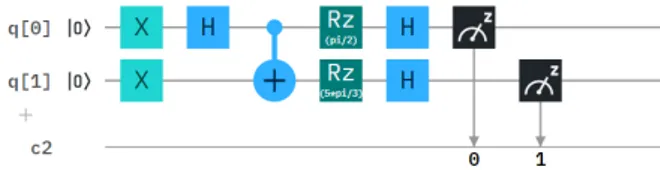
FIG. 2: Quantum circuit implemented in the IBM-QE quan-tum computer to measure the value E(ˆb, ˆc). The particular values of the rotations Rzaround the z axis correspond to the
the angles θˆb,ˆc= π
3 and θˆa,ˆc= 2π
3 .
A. Bell’s original inequality
First, we are going to test Bell’s inequality on the sin-glet state∣Ψ−⟩, for which we expect the violation of Bell’s inequality. The quantity E(ˆa,ˆb) stands for the the prod-uct of the outcomes of measuring the spin of the first qubit in the direction⃗a and the spin of the second in di-rection ˆb. For simplicity we will consider all directions in the x− y plane and the vector ˆa in the x direction. The quantum-mechanical calculation of E(ˆa,ˆb) for the singlet state provides
E(⃗a,⃗b)QM= ⟨Ψ−∣⃗σ ⋅ ˆa ⊗ ⃗σ ⋅ ˆb∣Ψ−⟩ = − cos θˆa,ˆb, (15) where θˆa,ˆbis the angle between the vectors ˆa and ˆb. The calculations for E(ˆa, ˆc) and E(ˆb, ˆc) proceed in a similar way. Substituting these results in Eq. (13) leads to the following inequality
∣ cos(θˆa,ˆc) − cos(θˆa,ˆb)∣ + cos(θˆb,ˆc) ≤ 1. (16) A graphical representation of the left side of Eq. (16) shows that the inequality is violated in the wide region of Fig. 1 depicted with black colour.
In the next step, we want to test this inequality using the IBM-QE quantum computer. To this end, we explore the inequality along a line of the Fig. 1 by fixing the value of the angle θˆb,ˆc= π3 and varying θˆa,ˆb.
In Fig. 2, we show the circuit to measure E(ˆb, ˆc). First, we prepare the singlet state starting from the two-qubit ∣00⟩ by applying a X gate to each single qubit. After that, we use a Hadamard gate acting on the first qubit and finally we apply a CN OT gate to the two-qubit state with the first qubit as a control. This last gate will flip the spin of the second qubit when the first qubit is in the state∣ 1⟩. Once the singlet state is prepared, we measure the spin of each qubit along the desired directions. In a similar way as we did for measuring the spin of single qubit in the x direction (see Eq.(9)), we evaluate the mean value of the tensor product of the operators measuring the spin of each qubit in the chosen directions. As these directions are on the x− y plane, we only need to rotate the qubit around the z axes with Rz = U1(λ) gate (where λ is the angle of rotation around the z axis) followed by a
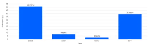
FIG. 3: Probabilities of the different basis states in which the two-qubit state is decomposed. These probabilities are used to calculate E(ˆb, ˆc). They collect the statistics of 8192 shots in the ibmqx2 processor of the IBM-QE.
Hadamard gate and the measurement of the third spin component, M(λ) = (HRz(λ))†SzHRz(λ) = ( 0 eiλ e−iλ 0 ) , (17) then E(ˆb, ˆc) = ⟨ψ−∣M (λ′) ⊗ M (λ))∣ ψ−⟩ = − cos (λ − λ′) . (18) Similar procedures are used to calculate E(ˆa, ˆc) and E(ˆa,ˆb), which are simpler because we assume ⃗a along the x-axis. Running this circuit many times (we use 8192 shots) the quantum computer provides the prob-abilities of the different possible states of two qubits in the z-basis. One example is shown in Fig. 3. With these probabilities we can compute the mean value E(ˆb, ˆc). To do this, we perform the summation of the products of the eigenvalues of the tensor product of Sz of each product state, 1 for ∣00⟩ and ∣11⟩ , and −1 for ∣10⟩ and ∣01⟩, by their respective probabilities. Using the circuit of Fig. 2 for each mean value we can calculate the left side of Bell’s inequality. The experimental results provided by the different runs in the IBM-QE, for different angles θˆa,ˆb keeping θˆb,ˆc= π/3 fixed, are shown in Fig. 4. The exper-imental data follow very well the theoretical calculations (purple line in Fig. 4). We observe several regions of θˆa,ˆb that violate Bell’s inequality with a maximum value of 1, 239 for θˆa,ˆb= θˆb,ˆc= π3.
B. CHSH inequality
The CHSH inequality does not assume any restriction in the state and we will test it for the four Bell’s states (Eq. (12)). For the states ∣Φ+⟩ and ∣Ψ−⟩ we choose as testing directions (Eq. (14)), ˆa and ˆa′ along the axes x and z which correspond to operators X and Z re-spectively and the directions ˆb = ˆw ≡ √1
2(ˆz + ˆx) and ˆb′ = ˆv ≡ √1
2(ˆz − ˆx) are represented by the operators W = √1
2(Z + X) and V = 1 √
2(Z − X). However, for the states∣Ψ+⟩ and ∣Φ−⟩ we change ˆb → ˆv and ˆb′→ ˆw.
The theoretical calculations of the different mean values for the state∣Φ+⟩ provide the following results
⟨Φ+∣Z ⊗ W ∣Φ+⟩ =√1
2, ⟨Φ
+∣Z ⊗ V ∣Φ+⟩ =√1
2, (19)
FIG. 4: Results of the left hand side of Bell’s inequality for the singlet state, for a fixed θˆb,ˆc=
π
3 as a function of θa,ˆˆb. The
continuous purple line shows the theoretical quantum calcula-tion while the green crosses stand for the experimental results collecting three runs of 8192 shots each. The discontinuous line indicates the threshold for the evolution of Bell’s inequal-ity. Points above the line violate Bell’s inequalinequal-ity.
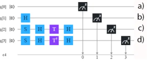
FIG. 5: Circuits to obtain the Bell’s states, a) is the Ψ−
state, b) is the Ψ+
state, c) is the state Φ−
and d) is the circuit for the state Ψ+
⟨Φ+∣X ⊗ W ∣Φ+⟩ =√1
2, ⟨Φ
+∣X ⊗ V ∣Φ+⟩ = −√1 2. (20) Therefore the left side of the CHSH inequality (Eq. (14)) is 2√2, which violates the inequality. Similar procedure using the corresponding directions for each Bell’s state provides us the same result for the left side of the CHSH inequality
Next we will test the inequality for the different Bell’s states using the IBM-QE. To this end, we build the Bell’s states, starting from the 2-qubit state∣00⟩, using the cir-cuits shown in Fig. 5. Then, we orientate each qubit depending on the mean value we want to calculate as specified in Fig. 6. The measurement in the X and Y directions have been explained above. To measure along the direction W , we use the gates S− H − T − H,
(HT HS)†SzHT HS= 1 √ 2( 1 1 1 −1) = 1 √ 2(X + Z), (21) while for the direction V, we use the gates S−H −T†−H
(HT†HS)†S zHT†HS= 1 √ 2( 1 1 1 −1) = 1 √ 2(X +Z). (22) The proper combination of the circuits followed by the calculations of the mean values in the z-basis provide
FIG. 6: Gates which measure the spin of a qubit along the directions a)ˆz, b) ˆx, c) ˆw and d) ˆv. These gates are to be properly combined to measure the expectation values given in Eqs. (19-20)
the results shown in Table 1, for the different pieces con-tributing to the left side of the CHSH inequality.
State ZV ZW XV XW C
Ψ+ -0,476 -0,557 -0,569 0,621 2,22±0,02
Ψ− -0,463 -0,543 0,672 -0,524 2,20±0,02
Φ− 0,676 0,705 0,690 -0,520 2,59±0,02
Φ+ 0,746 0,621 -0,403 0,752 2,52±0,01
TABLE I: Contributions of each piece to the total left side of the CHSH inequality (column C) for the different Bell states, obtained with three runs of 8192 shots.
As expected, all Bell’s states violate the inequality be-cause they are entangled states. In order to clarify the relationship between the entanglement and the violation of the CHSH inequality, we will test the inequality for the product state ∣00⟩. For this state, we obtain as a mean value of each tensor product, the product of the mean values on each qubit. To maximise the left side of the inequality we choose ˆa, ˆa′, ˆb and ˆb′ along ˆx, ˆz, ˆv and ˆw respectively. The evaluation of the mean values on the state∣00⟩ is ⟨XV ⟩ = 0, ⟨XW ⟩ = 0, ⟨ZV ⟩ =√1 2, ⟨ZW ⟩ = 1 √ 2. (23) Combining these expectation values we obtain for left side of the inequality the value √2 which fulfils the in-equality, as was expected for a non entangled state.
Ap-plying the circuits of the Fig. 6 for three runs of 8192 shots in the IBM-QE we obtain C= 1, 54 ± 0, 01 in good agreement with the theoretical calculation.
IV. SUMMARY AND CONCLUSIONS
In this work we have explored the violation of the orig-inal Bell’s inequality for the singlet 2-qubit state. First, we have performed a theoretical quantum calculation and show that Bell’s inequality is violated in agreement with the fact that the singlet is an entangled state. In a sec-ond step, we have experimentally tested the inequality by using the IBM-QE. The experimental measurements are in agreement with the quantum calculations and the dis-crepancies should be attributed to poor statistics or most probably to the lost of coherence in running the quantum computer. Moreover, we have also studied the CHSH in-equality which was established for a wider set of states. We have calculated this inequality for the different Bell’s states and experimentally measured by using the IBM-QE. To clarify that entanglement is the key reason for the violation of these inequalities we have calculated and measured the inequality for a simple product state, show-ing that the inequality is fulfilled in this case, both for the theoretical quantum calculation and the experimen-tal measurement.
Bell-type inequalities are based on locality. However, entanglement, which is at the heart of quantum mechan-ics, produces non-local correlations between the differ-ent parts of a quantum system. This non-local character manifests in the violation of these inequalities. The pos-sibility to build and manipulate entangled states in the IBM-QE quantum computer opens cheap and new possi-bilities to test the basic principles of quantum mechanics.
Acknowledgments
I would like to show my gratitude to Dr. Artur Polls and Dr. Bruno Juli´a-D´ıaz for their guidance and advice.
[1] Einstein, A., B. Podolsky, and N. Rosen, Phys. Rev. 47, 777 (1935).
[2] Bell, J.S. Physics Physique Fizika, 1, 195 (1964).
[3] A.Aspect, P. Grangier,and G. Roger, Phys. Rev. Lett. 49, 91 (1982).
[4] John F. Clauser, Michael A. Horne, Abner Shimony, and Richard A. Holt. Phys. Rev. Lett. 23,880 (1969).
[5] D. Garc´ıa-Mart´ın, and G. Sierra. Journal of Applied
Math-ematics and Physics 6, 1460 (2018).
[6] J. S. Bell, Introduction to the hidden variable question, Proceedings of the International School of Physics ’Enrico Fermi’, Course IL, Foundations of Quantum Mechanics 171–81 (1971).
[7] IBM. IBM Quantum Experience. Retrieved from https://quantum-computing.ibm.com .