Scalable Similarity Matching in Streaming Time Series

DISI - Via Sommarive 14 - 38123 Povo - Trento (Italy)

http://www.disi.unitn.it

SCALABLE SIMILARITY MATCHING

IN STREAMING TIME SERIES

Alice Marascu, Suleiman Ali Khan, Themis

Palpanas

December 2011

Technical Report # DISI-11-484

This work has been published in PAKDD 2012. Please

reference as follows: Alice Marascu, Suleiman Ali Khan,

Themis Palpanas. Scalable Similarity Matching in Streaming

Time Series. Pacific-Asia Conference on Knowledge

Scalable Similarity Matching in Streaming Time Series

Alice Marascu University of Trento marascu@disi.unitn.eu

Suleiman Ali Khan Aalto University suleiman@cis.hut.fi

Themis Palpanas University of Trento themis@disi.unitn.eu

Abstract— Nowadays online monitoring of data streams is essential in many real life applications, like sensor network monitoring, manufacturing process control, and video surveillance. One major problem in this area is the online identification of streaming sequences similar to a predefined set of pattern-sequences.

In this paper, we present a novel solution that extends the state of the art both in terms of effectiveness and efficiency. We propose the first online similarity matching algorithm based on Longest Common SubSequence that is specifically designed to operate in a streaming context, and that can effectively handle time scaling, as well as noisy data. In order to deal with high stream rates and multiple streams, we extend the algorithm to operate on multilevel approximations of the streaming data, therefore quickly pruning the search space. Finally, we incorporate in our approach error estimation mechanisms in order to reduce the number of false negatives.

We perform an extensive experimental evaluation using forty real datasets, diverse in nature and characteristics, and we also compare our approach to previous techniques. The experiments demonstrate the validity of our approach.

Keywords: data stream, online similarity matching, time series

1.

Introduction

In the last years, due to accelerated technology developments, more and more applications have the ability to process large amounts of streaming time series in real time, ranging from manufacturing process control and sensor network monitoring to financial trading [1] [2] [3]. A challenging task in processing streaming data is the discovery of predefined pattern-sequences that are contained in the current sliding window. This problem finds multiple applications in diverse domains, such as in network monitoring for network attack patterns, and in industrial engineering for faulty devices and equipment failure patterns. Previous work on streaming time series similarity [4] [5] proposed solutions that are limited either by the flexibility of the similarity measures, or by their scalability (these points are discussed in detail in Section 2).

Motivated by these observations, in this paper we propose a new approach that overcomes the above drawbacks. First, we observe that in the absence of a time scaling constraint, degenerate matches may be obtained (i.e., by matching points in the time series that are too far apart from each other). In order to address this problem, we introduce the notion of the Continuous Warping Constraint that specifies the maximum allowed time scaling, and thus, offers only meaningful results.

We propose the first adaptation of the Longest Common SubSequence (LCSS) similarity measure to the streaming context, since it has been shown that LCSS is more

robust to noise (outliers) in time series matching [6].

In order to enable the processing of multiple streams, we introduce a framework based on Multilevel Summarization for the patterns and for the streaming time series. This technique offers the possibility to quickly discard parts of the time series that cannot lead to a match. Our work is the first to systematically study the required sliding window sizes of these multilevel approximations, as well as take into account and compensate for the errors introduced by these approximations. Therefore, we avoid false negatives in the final results.

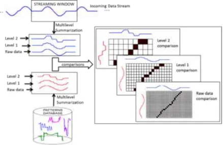
Figure 1 is a schematic illustration of our approach. The streaming time series subsequences included in the current streaming window are summarized using a multilevel summarization method and the same operation is performed on the predefined pattern sequences. Then, the different levels of these summaries are compared using a streaming algorithm with very small memory footprint.

The main contributions of this paper can be summarized as follows.

 We propose the first method that employs the LCSS distance measure for the problem of time series similarity matching and is specifically designed to operate in a streaming context.

 We introduce the Continuous Warping Constraint for the online processing setting in order to overcome the unlimited time scaling problem.

 We describe a scalable framework for streaming similarity matching, based on streaming time series summarization. We couple these techniques with analytical results and corresponding methods that compensate for the errors introduced by the approximations, ensuring high precision and recall with low runtimes.

Figure 1: Data stream monitoring for predefined patterns

 Finally, we perform an extensive experimental evaluation with forty real datasets. The results demonstrate the validity of our approach, in terms of quality of results, and show that the proposed algorithms run (almost) three times faster than SPRING [7] (the current state of the art).

The rest of the paper is organized as follows. We start by briefly presenting the background and the related work in Section 2. Section 3 presents our approach and describes in detail our algorithm. Section 4 discusses the experimental evaluations, and Section 5 concludes the paper.

2.

Background and Related Work

We now introduce some necessary notation, and discuss the related work.

A time series is an ordered sequence of n real-valued numbers T=(t1, t2, …, tn). We

consider t1 the first element and tn the last element of the time series. In the streaming

case, new elements arrive continuously, so the size of the time series is infinite. In this work, we are focusing on a sliding window of the time series, containing the latest k streaming values. We also define a subsequence ti,j of a time series T=(t1, t2, …, tn) is

ti,j=(ti, ti+1, …, tj), such that 1≤i≤j≤n. We say that two subsequences are similar if the

distance D between them is less than a user specified threshold ε.

2.1.

Distance Measures

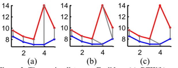
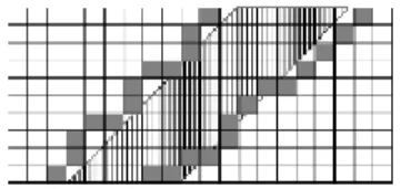
The most frequently used distance measure is the Euclidean distance, which computes the square root of the sum of the squared differences between all the corresponding elements of the two sequences (Figure 2(a)). The Euclidean distance cannot be applied on sequences of different sizes, or for element temporal shifts and, in these cases, the optimal alignment is achieved by DTW (Dynamic Time Warping) [8] (Figure 2(b)). DTW is an elastic distance that allows an element of one sequence to be mapped to multiple elements in the other sequence. If no temporal bound is applied, DTW can lead to pathological cases [9] [10] where very distant elements are allowed to be aligned. To avoid this problem, temporal constraints can be added in order to restrict the allowed temporal area for the alignment; the most used such constraints are the Sakoe-Chiba band [11] and the Itakura Parallelogram band [12] (shaded area in Figure 3). The LCSS

measure [6] is also an elastic distance measure that has an additional feature compared to DTW: it allows gaps in the alignment. This feature can be very valuable in real applications, since in this way we can model noise, outliers, and missing values (Figure 2(c)).

(a) (b) (c)

Figure 2: Time series distances: Euclidean (a), DTW(b), and LCSS (c)

Figure 3: Sakoe-Chiba band (left) and Itakura Parallelogram (right).

2.2.

Similarity Matching

The Euclidean distance is used by [4] for identifying similar matches in streaming time series. This study proposes a technique, where the patterns to be matched are first hierarchically clustered based on their minimum bounding envelopes. Since this

2 4 8 10 12 14 2 4 8 10 12 14 2 4 8 10 12 14

technique is based on the Euclidean distance, it requires the sequences to be of the same size and is rather sensitive to noise and distortion [13]. As a solution, [7] presented the SPRING algorithm that computes the DTW distance in a streaming data context. This algorithm allows comparison of sequences with different lengths and local time scaling, but does not efficiently handle noise (outlier points). We elaborate more on SPRING in the next subsection.

The warping distance techniques are also studied by [14], who propose the Spatial Assembling Distance (SpADe), a new distance measure for similarity matching in time series. An R-tree is used to index the multi-dimensional patterns. Their approach allows incremental distance computation.

Stream-DTW (SDTW) is proposed by [5] with the aim of having a fast DTW for streaming times series. SDTW is updatable with each new incoming data sequence. Nevertheless, the experimental results show that it is not faster than SPRING. In [15] the LCSS distance was used to process data streams, but was not adapted for online operation in a streaming context, which is the focus of our paper.

Other related works to this topic focused on approximations, thus proposing approximate distance formula. One example is the method proposed by [16] that uses the Boyer Moore string matching algorithm to match a sequence over a data stream. This approach is limited in that it operates with a single pattern and a single stream at a time. A multi-scale approximate representation of the patterns is proposed by [17] in order to speed up the processing. Even though the above representations introduce errors, neither these errors nor the accuracy of the proposed technique are explicitly studied.

2.3.

SPRING Overview

The basic idea of SPRING (for more details see [7]) is to maintain a single, advanced form of the DTW matrix, called Sequence Time Warping Matrix (STWM). This matrix is used to compute the distances of all possible sequence comparisons simultaneously, such that the best matching sequences are monitored and finally reported when the matching is complete.

Each cell in the STWM matrix contains two values: the DTW distance d(t,i) and the starting time s(t,i) of sequence (t,i), where t=1,2,…n and i=1,2,…m are the time index in the matrix of the stream and of the pattern respectively. A subsequence starting at

s(t,i) and ending at the current time t has a cumulative DTW distance d(t,i), and it is the

best distance found so far after comparing the prefix of the stream sequence from time

s(t,i) to t, and the prefix of the pattern sequence from time 1 to i. On arrival of a new

data point in the stream, the values of d(t,i) and s(t,i) are updated using Equations (1) and (2). A careful implementation of the SPRING algorithm leads to a space complexity of O(m) and time complexity of O(mn), just like DTW.

d t,i

( )

d_best=min d t

(

)

(

)

(

)

 

























3.

Our Approach

In this section, we present two novel algorithms for streaming similarity matching called naiveSSM (naive Streaming Similarity Matching) and SSM (Streaming Similarity Matching).

The naiveSSM algorithm efficiently detects similar matches thanks to three features: it constrains the time scaling allowed in the matches, thus, avoiding degenerate answers; it handles outlier points in the data stream, by using LCSS; and it uses a special hierarchical summarization structure that allows it to effectively prune the search space. Although naiveSSM provides good results, it is not aware of the computation error introduced by the summarization method. SSM takes care of the computation error and improves the results by using a probabilistic error modeling feature.

3.1.

The naiveSSM Algorithm

3.1.1. CWC Bands (Continuous Warping Constraint bands)

We observe that the simple addition of a Sakoe-Chiba band for solving the problem of degenerate matches would not be enough, since not all matching cases would be detected. Figure 4 illustrates this idea; two sequences situated outside of the band, but

very near of its bounds, are not detected as matching because they are outside of the allowed area. The solution we propose is a novel formulation of Sakoe-Chiba band, which we call Continuous Warping Constraint (CWC band).

CWC band consists of multiple succeeding overlapping bands where each of these bands is bounding one possible matching sequence (Figure 5). More precisely, we

propose to associate a boundary constraint to each possible matching, and not a general allowed area (as in Figure 4). In this way, the CWC band provides more flexible bounds

that follow the matching sequences behavior. Figure 5 shows three CWC bands. The first

matching sequence (dark grey) falls within the first CWC band, while the second sequence falls in the third CWC band, hence both being successfully detected as matching. A single CWC band is an envelope created around the pattern (the left allowed time scaling value being equal to the right allowed time scaling value); the size of the envelope is a user-defined parameter. The CWC bands have the additional advantage that they can be computed with negligible additional cost.

Figure 4: Sakoe-Chiba band (shaded area), and two candidate matching sequences (dark grey) falling outside the constraint envelope.

Figure 5: The same two candidate matching sequences as Figure 4, and three overlapping CWC bands.

The CWC bands can be added to the SPRING algorithm, on top of the DTW. Due to lack of space, in the following, we only discuss the application of CWC on top of streaming LCSS.

3.1.2. LCSS in a Streaming Context

LCSS provides a better support for noise compared to DTW, as we mention in Section 2. Equation (3) shows the LCSS computation of two sequences, A and B, of length n and m, respectively. The parameter γ is a user-defined threshold for the accepted distance. We now derive a novel formula for the streaming version of LCSS.

LCSS( A, B)= 0 if A or B is Empty

(

)

(

)

Since LCSS and DTW have similar matrix-based dynamic programming solutions (for the offline case), one may think that they also share the idea of the STWM matrix, thus, leading to a simple solution of replacing DTW with LCSS in the SPRING framework. Unfortunately, this is not a suitable solution: simply plugging LCSS Equation (3) into SPRING introduces false negatives and degenerate time scaled matches. The false negatives occur because the otherwise clause in Equation (3) selects the maximum of the two preceding sequences irrespective of the portion of the δ time scaling they have consumed. Therefore, it is possible that the selected sequence may have a higher LCSS value than the discarded sequence, but has already exceeded its allowed time scaling limit. The problem is that even though such a sequence will never become a matching sequence (because of its length), it may prevent a valid sequence from becoming a match.

To address this problem, we formulate the new CWC band constrained LCSS Equation (4) (due to lack of space, we omit the intermediate steps of deriving these new equations). In Equation (4), δ is a user defined parameter defining the maximum time scaling limit for the CWC bands, which corresponds to the size of the bands. The LCSS count is incremented only if the current pattern and stream value match, that is, they have a point to point distance less than the threshold γ, and the preceding diagonal LCSS falls within the CWC band (i.e., belongs to the allowed envelope area). Equation (5) describes the corresponding update of the starting time.

l(t,i)= 1+l(t-1,i-1) if dist a

( )

(

)

(

(

)

)

(

(

)

)

(

(

)

)

When trying to identify candidate matches of a given pattern in a streaming time series, we are bound to waste a significant amount of computations on testing subsequences that in fact cannot be a solution. In this subsection, we describe how we can effectively prune the search space by using a multilevel summarization structure on top of the

      ( 1, 1) ( , ) ( 1, 1) ( , ) ( 1, ) ( , ) ( 1, ) ( , 1) ( , ) ( , 1) s t i if l t i l t i s t i s t i if l t i l t i s t i if l t i l t i             _{  } 

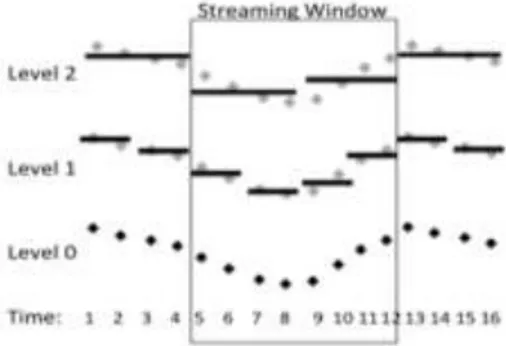
streaming time series. Figure 6 illustrates the idea of a multilevel hierarchical summary

(levels 1 and 2 in this figure), depicted in black-colored lines, of a streaming time series (level 0), depicted in black-colored points.

In this study, we use PAA1 _{[18] as a summarization method, because of its simplicity,}

effectiveness, and efficiency in a streaming environment. However, other summarization methods can also be used. The algorithm operates in an incremental fashion. It processes the incoming values in batches and waits till the number of data points received is sufficient to build a complete new top level approximation segment, at which point the approximations of all levels are computed at once.

The benefit of employing this hierarchical summary structure is that the similarity matching can be executed on the summaries of the streaming time series, instead of the actual values, whose size is considerably larger. If the algorithm finds a candidate match at a high level of approximation, then it also checks the lower levels, and if necessary the actual stream as well.

Note that since we are using an elastic distance measure (i.e., LCSS), it is possible that the matching at lower approximation levels, and especially at the actual pattern or stream, may yield different starting and ending points. If not treated properly, this situation may lead to false negatives.

Figure 6: Multilevel Summarization

Figure 7: Sequence Placement in Streaming Window at t δ

First of all, the window size must be at least as big as the searched pattern. Then, since we use elastic matching, a candidate matching sequence can be extended up to δ data points in both directions (i.e., to the left and right), which gives the following inequality for the window size (refer to area “A” in Figure 7): WindowSize ≥

patternLength + 2δ. When a candidate matching sequence is detected, we must

determine its locally optimal neighbour. For this purpose, and since δ is the maximum allowed time scaling, the window has to contain an extra δ data points (depicted as “B”

in Figure 7). Finally, one more data point is needed for the optimality verification of the

candidate sequence. The above statements lead to the following inequality for the window size: WindowSize = patternLength +3 δ +1.

1 _{PAA (Piecewise Aggregate Approximation) divides the time series into N equal segments and approximates}

3.2.

SSM algorithm

3.2.1. Probabilistic Error Modelling

As all approximations result in loss of information, multilevel summarization is also expected to lead to some loss of information. Therefore, it is highly probable that the set of candidate matches found at the highest level may not contain all the actual matches. One way of addressing this problem is by lower bounding the distance of the time series. Even though this is possible, this approach would lead to a computationally expensive solution. Instead, we propose an efficient solution based on the probability with which errors occur in our distance computations.

We randomly choose a sample of actual data point sequences from the streaming window. For all the sequences in the sample, we compute the error in the distance measure introduced by the approximation (by comparing to the distance computed based on the raw data). Then, we build a histogram that models the distribution of these errors, the Error Probability Distribution (EPD). Evidently, errors are smaller for the lower levels of approximation, since they contain more information, and are consequently more accurate than the approximations at higher levels.

The pruning decision of a candidate matching sequence is based on the EPD: we define the margin as 1-3σ (standard deviations) of the EPD. Intuitively, the error-margin indicates the difference that may exist between the distance computation based on the summarization levels and the true distance. Using an error-margin of 3σ, we have a very high probability that we are going to account for almost all errors.

Then, if the distance of a candidate sequence computed at one of the approximation levels is larger than the user-defined threshold ε, but less than ε + error-margin, this sequence remains a candidate match (and is further processed by the lower approximation levels).

3.2.2. Change-Based Error Monitoring

The data stream characteristics change continuously over time and EPD must reflect them. For this purpose, we set up a technique allowing the effective streaming computation of EPD. The most expensive part of the EPD computation is the computation of the LCSS distance between the pattern and all the samples. The continuous computation of EPD can be avoided by setting up a mechanism that will trigger the EPD re-computation only when the data distribution changes significantly.

In the work, we propose to use a technique that is based on the mean and variance of the data. This technique was proven to be effective [19] [20] and can be integrated in a streaming context. Though, more complex techniques for detecting data distribution changes can be applied as well [21].

Our algorithm operates as follows. When sufficient data arrives in the stream window, the EPD is constructed. Then the mean and the variance of the original streaming data are computed and registered together with the error margins. We consider that the EPD needs to be updated (i.e., reconstructed), only when the mean and variance of the current window changes by more than one standard deviation compared to the previous value. We will call this technique change-based error monitoring.

The only remaining question to answer is how often to sample. If we look for a pattern of size k within a streaming window of size n, there are (n – k + 1) possible matching sequences for the first element of the window, (n – k + 1 - 1) possible matching sequences for the second element of the window and so on until there is 1

single possible matching sequence for the n-k element of the window. Therefore there are (n–k+1)+(n–k+1-1)+(n–k+1-2)+...+1=(n–k+1)*(n–k+2)/2 possible matching sequences.

Given the large number of possible matching sequences, even a very small sampling rate (i.e., less than 1%) can be sufficient for the purpose of computing EPD. In the following section, we experimentally validate these choices.

4.

Experimental Evaluation

All experiments were performed on a server configured with 4xGenuine Intel Xeon 3.0 GHz CPU, and 2 GB RAM, running the RedHat Enterprise ES operating system. The algorithm was coded in Matlab.

We used forty real datasets with diverse characteristics from the Time Series Repository [22] of the University of California, Riverside2. Patterns are randomly extracted from the streams, and the experiments are organized as follows. A dataset consists of several streams and several patterns. An experiment carried out on a single dataset means that each pattern in that dataset is compared with each stream in the same dataset. All experiments are carried out with patterns of length 50 (unless otherwise noted), and we report the averages over all runs, as well as the 95% Confidence Intervals (CIs).

We use precision and recall to measure accuracy: precision is defined as the ratio of true matches over all matches reported by the algorithm; recall is the ratio of true matches reported by the algorithm over all the true matches.

Due to lack of space, we only report the most important experimental results. All the results, as well as a detailed description of the algorithms, including the SSM version with DTW and all the pseudocodes, can be found in the full version of this paper3_.

4.1.

Approximate Similarity Matching

We first examine the performance of the naiveSSM algorithm. In this case, we use up to 5 levels for the multilevel summarization. The performance when using only some of these 5 levels of the summarization is lower (these results are omitted for brevity). This is because level skipping results in more matches to be processed at lower levels, where processing is more expensive. We also did not observe any significant performance improvements when considering more than 5 levels.

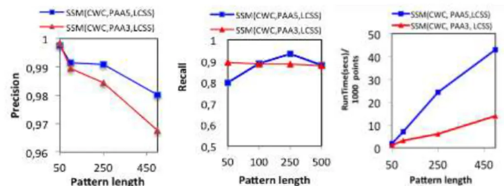
Figure 8 shows the precision, recall and runtime of naiveSSM as a function of the

pattern size, which ranges from 50 to 500 data points. We report results for naiveSSM for the cases where we have 3 (PAA3) and 5 (PAA5) approximation levels. We observe that naiveSSM scales linearly with the length of the patterns. The precision and recall results show that even though precision remains consistently high (averaging more than 98%), recall is rather low: naiveSSM using LCSS averages a recall of 90%.

These results confirm that the errors introduced by the approximation may lead to some matches being missed. Precision numbers are nevertheless high, because every candidate match is ultimately tested using the raw data as well. Finally, the results show that using 5 levels for the summarization leads to higher accuracy, but also higher

2 _{A detailed list of the datasets we used is available as an anonymous online resource:}

http://tinyurl.com/42vlss5

running times (Figure 8(right)).

Figure 8: Precision (left), Recall (middle), and Run Time (right) for different variants of naiveSSM.

4.2.

Compensating for Approximation Errors

We now present results for SSM, which aims to compensate for the errors introduced by the multilevel summarization, and thus, lead to higher recall values.

Table 1 shows the precision and recall numbers achieved by SSM with continuous and with change-based error monitoring, as a function of the error-margin. The results show that precision is in all cases consistently above 99%, while recall is over 95%, a significant improvement over naiveSSM. We also observe that SSM with change-based error monitoring performs very close to SSM with continuous monitoring (which is much more expensive). This validates our claims that the change-based error monitoring is an effective and efficient alternative to continuous error monitoring for producing high quality similarity matches. Finally, we observe that by increasing the error-margin from 1σ to 3σ, recall is only slightly improving. As expected, precision is unaffected.

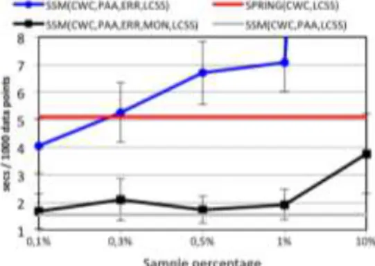
We now study the role of the sampling rate on performance. Remember that this is the rate at which we sample the stream sequences during change-based error-monitoring, for computing the distance error introduced by the approximation and for building the EPD. In these experiments, we used an error-margin of 1σ, and sampling rates between 0.1% and 10%. Figure 9 presents the runtime of SSM as a function of the

sampling rate. The results demonstrate that SSM with change-based error monitoring (curve with black squares) runs almost three times faster than the current state of the art (red, constant curve): SPRING (for fairness, with LCSS and CWC bands). Note that the time performance of SSM with continuous error monitoring (curve with dark blue circles) is better than only for very low sampling rates (0.1%).

It is also interesting to note that SSM performs very close to the lower bound represented by the naiveSSM algorithm (light grey curve), which does not use any error monitoring at all, and suffers in recall, averaging less than 90% (refer to Figure 8). In

contrast, SSM achieves a significantly higher recall value, more than 95% (refer to Table 1). We note that the precision and recall of SSM with change-based monitoring remain stable, 99% and 96%, respectively, as the sampling rate varies between 0.1%-10% (results omitted for brevity). Overall, we can say that the SSM algorithm with change-based error monitoring is not only time efficient, but also highly accurate even when the error margin is small (1σ).

In the final experiment, we measure the number of distance computations performed by SSM with change-based error monitoring, using 3 levels of summarization. (Changing the sampling rate between 0.1%-10% does not affect the results.) We measured separately the number of computations for each level of summarization, including level 0: the raw data. The results show that the largest percentage of computations, 66%, occur at level 0 (18% at level 1, 12% at level 2, and 4% at level 3). These results signify that future attempts to further improve the runtime of the algorithm should focus on techniques for more aggressive, early (i.e., at higher levels) pruning of the candidate sequences.

SSM continuous change-based SSM error- margin Pr R Pr R 1σ 0.99 0.95 0.99 0.95 2σ 0.99 0.96 0.99 0.96 3σ 0.99 0.97 0.99 0.96 Table 1: Precision and Recall for SSM with continuous and change-based error monitoring, as a function of the error margin.

Figure 9: Runtime vs Sample Percentage for SSM

5.

Conclusions

Similarity matching in streaming time series has recently attracted lots of interest. In this work, we propose a new algorithm, able to efficiently detect similarity matching in a streaming context that is both scalable and noise-aware.

Our experiments on forty real datasets show that the proposed solution runs (almost) three times faster than previous approaches. At the same time, our solution exhibits high accuracy (precision and recall more than 99% and 95%, respectively), and ensures that we do not obtain degenerate answers, by employing the novel CWC bands.

6.

References

[1] "Airoldi E., Faloutsos C., Recovering latent time-series from their observed sums: network tomography with particle filters, KDD 2004".

[2] " Borgne Y.-A. L., Santini S., Bontempi G., Adaptive model selection for time series prediction in wireless sensor networks. Signal Process, 87(12):3010–3020 2007".

[3] "Zhu Y., Shasha D., Statstream: statistical monitoring of thousands of data streams in real time, VLDB 2002".

[4] "Wei, L., Keogh, E. J., Herle, H. V., and Neto, A. M. Atomic Wedgie: Efficient Query Filtering for Streaming Times Series. ICDM 2005, 490-497".

Knowledge Engineering (62) 2007, 438–458".

[6] "Vlachos, M., Gunopulos, D., and Kollios, G. Discovering similar multidimensional trajectories. ICDE 2002, 673–684".

[7] "Sakurai, Y., Faloutsos, C., and Yamamuro, M. Stream Monitoring under the Time Warping Distance. ICDE 2007".

[8] "Ratanamahatana, C. A., and Keogh, E. Everything you know about Dynamic Time Warping is Wrong, Third Workshop on Mining Temporal and Sequential Data, 2004".

[9] "Ding, H., Trajcevski, G., Scheuermann, P., Wang, X., and Keogh, E. Querying and Mining of Time Series Data: Experimental Comparison of Representations and Distance Measures, VLDB 2008".

[10] "Stan Salvador and Philip Chan, FastDTW: Toward Accurate Dynamic Time Warping in Linear Time and Space, in Intelligent Data Analysis 11(5), 2007 561-580".

[11] "Sakoe, H. and Chiba, S. Dynamic programming algorithm optimization for spoken word recognition, ASSP 1978".

[12] "Itakura, F. Minimum Prediction Residual Principle Applied to Speech Recognition, ASSP-23, 1975, 52-72".

[13] "Agrawal, R., Faloutsos, C., and Swami, A. N. Efficient Similarity Search in Sequence Databases. FODO 1993, 69-84".

[14] "Chen, Y., Nascimento, M. A., Ooi, B. C., and Tung, A. K. H. SpADe: On Shape-based Pattern Detection in Streaming Time Series. ICDE 2007".

[15] "Marascu A., Masseglia F., Mining Sequential Patterns from Data Streams: a Centroid Approach, J. Intell. Inf. Syst. Volume 27, number 3, 2006, pages 291-307".

[16] "Harada, L. Detection of complex temporal patterns over data streams. Information Systems 29(6) 2004, 439–459".

[17] "Lian, X., Chen, L., Yu, J. X., Wang, G., and Yu, G. Similarity Match Over High Speed Time-Series Streams. ICDE 2007".

[18] "Keogh E. J., Chakrabarti K., Pazzani M.J., and Mehrotra S., Dimensionality Reduction for Fast Similarity Search in Large Time Series Databases. Knowl. Inf. Syst., 3(3), 2001.".

[19] "Babcock, B., Datar, M., and Motwani, R. Sampling From a Moving Window Over Streaming Data, SODA, 2002".

[20] "Babcock, B., Datar, M., Motwani, R., and O’Callaghan, L. Maintaining Variance And k-medians Over Data Stream Windows PODS, 2003, 234–243".

[21] "Ben-David, S., Gehrke, J., and Kifer, D. Identifying Distribution Change in Data Streams. In VLDB, Toronto, ON, Canada, 2004".

[22] "UCR: Time Series Data Archive. http://www.cs.ucr.edu/~eamonn/time_series_data/".