UNIVERSITY
OF TRENTO
DIPARTIMENTO DI INGEGNERIA E SCIENZA DELL’INFORMAZIONE
38123 Povo – Trento (Italy), Via Sommarive 14
http://www.disi.unitn.it
NEW RESULTS ON ELECTROMAGNETIC IMAGING BASED ON
THE INVERSION OF MEASURED SCATTERED-FIELD DATA
R. Azaro, G. Bozza, C. Estatico, A. Massa, M. Pastorino, D. Pregnolato,
and A. Randazzo
January 2011
New results on electromagnetic imaging based on the inversion of synthetic and
measured scattered-field data
R. Azaro,
1G. Bozza,
2C. Estatico,
3A. Massa,
4M. Pastorino,
2D. Pregnolato,
4and A. Randazzo
21 EMC S.r.l., via Greto di Cornigliano 6r – 16152 Genova, Italy. Phone: +390106017025 e-mail: [email protected]
2 Department of Biophysical and Electronic Engineering, University of Genoa, Via Opera Pia 11A, 16145, Genova, Italy.
Phone: +39 010 3532242 Fax: +39 0103532245 e-mail: [email protected], [email protected], [email protected]
3 Department of Mathematics, University of Genoa,
Via Dodecaneso 35, 16146 Genova, Italy e-mail: [email protected]
4 Department of Information and Communication Technology, University of Trento
Via Sommarive 14, I-38050 Trento, Italy. Phone: +39 0461882057 Fax: +39 0461881696 e-mail: [email protected]
Abstract – A new approach for the inversion of synthetic and measured scattered data is proposed in this paper. The approach is based on
an iterative technique in which the nonlinear equations of the inverse scattering problem are solved within the p-th order Born approximation. A regularization scheme based on an Inexact-Newton method is applied. Several numerical simulations and experimental results are reported. Multiple separated dielectric cylinders are localized and reconstructed in a noisy environment.
Keywords – Imaging Systems, Microwaves, Electromagnetic Scattering, Inverse Problems
I. INTRODUCTION
The research activity concerning the development of new and efficient imaging systems is in rapid progress. New imaging technologies are continuously proposed, improved and combined with the existing ones [1].
Among the various new approaches, electromagnetic diagnostic techniques are facing an increasing number of potential applications, including the detection of tunnels, pipes and other buried inhomogeneities, civil and industrial nondestructive tests and medical diagnostics [2]-[6].
In these techniques, incident electromagnetic waves are used to interrogate an object. Then, the perturbed field (the scattered field) is collected by one or more sensors in a certain number of locations outside the object. If cylindrical objects are considered and the illuminating/receiving system rotates around the cross section of the object, tomographic information is collected.
The goal is usually to retrieve the dielectric profile of the object or to inspect it in order to detect cracks or defects inside the material.
From a mathematical point of view, electromagnetic imaging approaches are based on the inverse scattering problem, whose equations constitute the relationships between the unknown parameters of the targets and the "input" data (i. e., samples of the scattered electric field, which are collected by a suitable measurement apparatus.)
The development of efficient imaging systems based on the electromagnetic scattering is still considered a difficult task. The main reason is related to the nonlinear nature of the equations of the inverse scattering problem. In addition, the ill-posedness of the problem makes the solution still more complicated, since specific "regularizations" must be applied. Finally, the computational load is usually another limiting factor that is, of course, not independent of the nonlinearity and ill-posedness.
Despite the above limiting factors, several microwave-imaging approaches have been recently proposed. In order to linearize the inverse scattering problem, simplified imaging methods have been developed under the first-order Born approximation [7]-[10]. Under this approximation, the total electric field, in the whole space, is written in terms of the known incident field (the unperturbed field).
Since the first-order Born approximation can be applied only for weakly scatterers, a certain improvement in the detection capabilities can be obtained by considering the second-order Born approximation [11][12]. In this case the problem becomes nonlinear, although the dielectric parameters remain the only unknowns to be determined.
It should be mentioned that, in recent years, several approaches have been proposed for the solution of the full nonlinear inverse scattering, which are able, in principle, to inspect very strong scatterers. They are mainly iterative methods, both deterministic and stochastic ones. However, despite the significant improvement achieved, these strategies are still quite complicated and very time consuming.
In the present paper, a new deterministic and iterative method is proposed. The approach is a two-step Inexact-Newton method, which is developed in the framework of the p-th order Born approximation.
converges, it is interesting to evaluate improvements that can be obtained by using higher-order approximations and the corresponding computational load.
The approach (described in Sections II and III) combines an outer iteration loop (Newton iteration) with an inner loop, in which the truncated Landweber method is applied. The method has very good regularization properties, as proven by the simulations that are reported in Section IV.
Finally, in Section V, preliminary experimental validations of the approach are provided. The input data for this experimental validation are measured in the anechoic chamber of the Joint Laboratory DIBE-EMC S.r.l., Genova, Italy. Furthermore, data provided by the Frésnel Institute, Marseilles, France, are used to test the method [13], too.
II. MATHEMATICAL FORMULATION
As it is well known, the inverse scattering problem consists in retrieving the electromagnetic properties of a region illuminated by one or more known sources, from the field measured outside the region itself.
The geometrical two-dimensional configuration of the considered imaging system is reported in Figure 1. The area under
test, , is illuminated from V different directions (multiview arrangement) and, for each view, the electric field is collected
at M points located in the domain , (
inv
Ω
obs
Ω Ωinv∩Ωobs=∅.)
Figure 1 – Geometrical configuration of the imaging system.
In this paper, transverse-magnetic illumination is adopted, that is, every source produces a known incident wave polarized
orthogonally to the plane in which lies. This hypothesis allows a scalar formulation of the problem in terms of the
projection along the z-axis of the involved fields. For this reason, we call and the electric field radiated by the v-th
source in free space and in presence of the scatterer, respectively, actually meaning their projections.
inv Ω ) (v inc E Etot(v)
Furthermore, without losing in generality, is supposed to be surrounded by vacuum, whose dielectric permittivity and
magnetic permeability are denoted by
inv
Ω
0
ε and μ . 0
Under these hypotheses and assuming that no magnetic media are involved, (v) and are related as follows
inc E Etot(v)
∫
Ω = − inv d G E j E E v tot v inc v tot( ) ( ) ( ') ( ') ( | ') ' ) ( 0 ) ( ) ( r r r r r r r ωμ τ , (1)where ω is the pulsation at which the fields oscillate, is the known Green’s function for the two-dimensional
Helhmoltz equation [14] and τ is the scattering potential defined by
) ' |
( rr
) 1 ) ( ( ) (r = jωε0 εr r − τ , (2)
being εr(r) the relative dielectric permittivity of Ω at point r. inv
By defining the scattered field () () (v), equation (1) can be written in operatorial form as
inc v tot v scatt E E E = − V v E E F v scatt v tot]( ) ( ) 1, , , [ () () K = = r r τ , (3)
where the nonlinear integral operator F is defined as follows
∫
Ω = inv d G E j E F v tot v tot]( ) ( ') ( ') ( | ') ' , [ () 0 ) ( r r r r r r ωμ τ τ . (4)In the inverse problem, the total electric field (ν)(r) in the investigation domain
tot
E Ω is as unknown as τ. Furthermore, inv
because of the measurement process, the electric field in Ωobs is corrupted by noise. Hence, the solution of the inverse
problem requires the inversion of the nonlinear integral equation
obs v scatt v tot E E F[ , ](r)= ()*(r), r∈Ω ) ( τ , (5)
where (v) * denotes the difference between the measured total electric field and the incident one.
scatt E
The nonlinear integral equation (5) is very critical and computationally expensive to solve. Moreover it is not sufficient to
determinate both τ and , , but only the so-called equivalent current density . In order to
overcome this problem, in this work the term is replaced by its p-th order Born approximation.
) ( ) (v r tot
E r∈Ωinv Jtot(v)(r)=τ(r)Etot(v)(r)
] , [ (v) tot E Fτ
The p-th order Born approximation allows the scattered field to be written in terms of the scattering potential τ and of the
known incident field . In this way, the knowledge of the total electric field in the investigation domain is not necessary.
In fact, the operator
) ( ) (v r inc E ] [ ~(v)τ p
F expressing the p-th order Born approximation is recursively defined by the following relations
∫
Ω = inv d G E j F v inc v[ ]( ) ( ') ( ') ( | ') ' ~ () 0 ) ( 1 τ r ωμ τ r r r r r (6)[
]
∫
Ω − + = inv d G F E j F v p v inc v p [ ]( ') ( | ') ' ~ ) ' ( ) ' ( ) ]( [ ~ () 1 ) ( 0 ) ( r r r r r r r ωμ τ τ τ . (7)By using this approximation, equation (5) becomes
obs v scatt v p E F~()[τ](r)= () *(r), r∈Ω , (8)
where the only unknown is the scattering potential τ. Since ~(v)
p
F is a composition of Fredholm integral operators on an infinite dimensional space, equation (8) is ill-posed [15].
Furthermore, for p>1 the problem turns out to be nonlinear.
Moreover, it is fundamental to remark that the sequence defined by relations (6) and (7) converges to the exact scattered field
for p→+∞ only if the scatterer is not too strong [7].
Among different mathematical tools, equation (8) is solved by using an iterative Newton method, in which at each step the
nonlinear ill-posed equation (8) is linearized by means of the Fréchet derivative of ~(v)
p
F . In fact, it is possible to write
) ( ) ]( [' ~ ) ]( [ ~ ) ]( [ ~ () 2 , ) ( ) ( τ σ τ σ σ τ O F F F v p v p v p + r = r + r + , (9) where '~() , v p
F τ is the Fréchet derivative of the operator F~p(v) at point τ, that is, the linear operator given by the following
∫
Ω ′ ′ ′ ′ = inv G E j F v inc v r r r r r r) ( ) ( ) ( | )d ]( [' ~ () 0 ) ( , 1τ σ ωμ σ (10)∫
∫
Ω − Ω − + + + + = inv inv d G h F j d G F h j h F h F v p v p v v p ' ) ' | ( ) ' ]( [ ~ ) ' ( ' ) ' | ( ) ' ]( [ ~ ) ' ( ) ]( [ ~ ) ]( [ ~ )' ( , 1 0 ) ( 1 0 ) ( 1 )' ( , r r r r r r r r r r r r τ τ τ ωμ τ ωμ (11)III. THE REGULARIZING INVERSION PROCEDURE
As already mentioned, the p-th order Born equation (8) is solved by means of a regularizing Inexact-Newton method. The method is based on the following iterative scheme: At any step, equation (8) is first linearized, and the generalized solution of such a linear equation is approximated and regularized by using an iterative method, namely the truncated Landweber method for linear systems. A regularizing scheme is required to solve the linearized equation because it results as ill-posed as the nonlinear one [15].
The algorithm can be summarized by using an outer-inner iterative scheme, where • any outer iteration is the Newton step for the linearization, and
• any inner iteration is the Landweber step for the regularized resolution of the linear equation arising from the outer step. The proposed method is able to improve the performances with respect to the widely used Landweber method for nonlinear inverse problems, in terms of numerical cost, and hence it can be considered as a valid tool for real applications. Indeed, the proposed method requires the computation of a limited number of Fréchet derivatives, which is generally the expensive part of any solving procedure by linearization.
If is a (suitable) initial guess which approximates the true object function τ, the Newton method can be
schematized as follows. ) ( 2 0∈L Ωinv τ
Let j = 0 and solve, for 2( ), the linear system
inv j∈L Ω σ V v F E F j v v scatt j v j ( ), 1,.., ~ ] [' ~ ( ) () * ) ( = − = τ σ τ , (12)
then update τj+1=τj +σj and repeat with j:= j+1, until a stopping rule is satisfied or when j = jmax.
At any Newton step, since the linear equation (12) is ill-posed, we search for a regularized solution by computing a fixed number of steps of the following truncated Landweber method.
Set σj,0=0 and let kmax be a maximum number of iterations. Initialized k=0 and chosen β such that j
1 1 * ~ ' ' ~ 2 0 () () − =
∑
< < s V v j v j v j F Fτ τ β , compute ] ) ) ( ~ ( ' ~ ' ~ ' ~ [ V 1 ) ( ) ( * * , * , 1 , ) ( ) ( ) (∑
= + − − − − = v j v v scatt k j j k j k j F E F F F v j v j v j σ τ β σ σ τ τ τ (13)then update k:= k+1 and repeat until k = kmax. Here
*
' ~( v)
j
Fτ denotes the adjoint operator of the Fréchet derivative '
~( v)
j
Fτ , and
s
⋅ is the spectral norm, that is, the largest modulus of the singular values of the argument.
The Landweber method (13) is an iterative regularization method, that is, an iterative method where the number of iterations plays the role of a regularization parameter. Indeed, in the case of noisy data, it can be easily proven that the first iterations provide noise filtering, while the subsequent ones restore from components with higher noise, so that the accuracy of the
iterative solution starts to become worse. The method requires the choice of two parameters: the convergence parameter βj and
Concerning βj, it is simple to show that the constraints 1 1 * ~ ' ' ~ 2 0 () () − =
∑
< < s V v j v j v j F Fτ τβ guarantee the convergence of σ j ,k
towards σ , for j k→+∞. In our tests, we always set
1 1 *~ ' ' ~() () − =
∑
= s V v j v j v j F Fτ τ β .Since kmax is the regularization parameter, in order to prevent the approximated solution σj,kmax to suffer from the noise on
, a quite small number of iterations is to be performed. In our experience, a good choice is kmax ≤ 10.
) (v
scatt
E
IV. NUMERICAL RESULTS
The proposed method has been tested by means of several numerical simulations. A single-frequency configuration is assumed. Furthermore, for all the targets considered in this section, the imaging configuration (Figure 1) is composed by V = 8 views, in which the sources are located at positions (in polar coordinates)
. ,..., 1 , 4 ) 1 ( , v v V R v ⎟ = ⎠ ⎞ ⎜ ⎝ ⎛ − = π s (14)
For each view, M measurement points are used. Such points lie on an arc of circumference of width 2π−Δθ radians. The
m-th measurement point at the n-th view has coordinates given by
⎟ ⎠ ⎞ ⎜ ⎝ ⎛ − +Δ + −Δ − = 2 ( 1) 2 ) 1 ( 4 , m M v R v m θ π θ π r . (15)
Moreover, in the numerical computation, the test area Ω is partitioned in to N square subdomains and both the field and inv
dielectric quantities are assumed to be constant in each subdomain.
The accuracy of the inversion algorithm is evaluated by using the following error parameters
∑
∈ − = obj N n n n n obj obj N e ε ε ε ε ~ # 1 (16)∑
∈ = obj N n n obj m r N 0 ~ # 1 ε ε ε (17)∑
∈ − = bg N n n n n bg bg N e ε ε ε ε ~ # 1 (18)∑
= − = N n n n n N e 1 ~ 1 ε ε ε ε (19)∑
= − = V v v meas tot v E tot e 1 2 ) ( ) ( ~ E E (20)where Nobj and Nbg are the sets of indexes corresponding to the subdomains which are occupied by the objects and the
background, respectively, #Nobj and #Nbg are the numbers of elements of Nobj and Nbg, respectively, ε and n ε~ are the actual n
and reconstructed values of the relative dielectric permittivity in the n-th subdomain, and meas(v) and
tot
E ~(v)
tot
E are the arrays
containing the actual and reconstructed values of the total electric field at the M measurement points for the v-th view.
Furthermore, in all the simulations, the following values for the parameters of the inversion algorithm are used: kmax = 5
and jmax = 20.
The first performed simulations have been intended to evaluate the influence of the order of the Born approximation on the target reconstruction. To this end, circular homogeneous cylinders of several dielectric permittivities have been reconstructed at
the operating frequency of 600 MHz.
In particular, cylinders of radius a = λ0/5 = 0.1m and of relative dielectric permittivity in the range [1.2, 3] are used.
The locations of the sources and of the receivers can be obtained from relations (14) and (15) by setting R=1.67m,
241 = M , and 3 π θ =
Δ . The input data are computed by an analytical expression of the scattered field [16] and they are
corrupted by a Gaussian noise with zero mean value so that the signal-to-noise ratio (SNR) is equal to 25 dB.
The investigation domain is a square plane region with side L = 2λ0 = 1 m, which is discretized in 25 × 25 square
subdomains. Table I reports the object reconstruction error obj, for the considered orders of the Born approximation.
eε
Table I – Errors on the dielectric reconstruction (eεobj ) of circular cylinders of radius a = λ0/5 and of different permittivity for several values of the p-th Born approximation. SNR = 25 dB. eεobj εobj p=1 p=2 p=4 p=6 p=8 1.2 0.055 0.048 0.047 0.047 0.047 1.4 0.098 0.077 0.069 0.069 0.069 1.6 0.15 0.11 0.092 0.090 0.090 1.8 0.21 0.16 0.13 0.11 0.11 2.0 0.26 0.20 0.19 0.20 0.14 2.2 0.32 0.24 0.24 0.25 0.17 2.4 0.38 0.28 0.27 0.33 0.30 2.6 0.44 0.31 0.29 0.36 0.36 2.8 0.48 0.34 0.30 0.27 0.39 3.0 0.54 0.37 0.35 0.34 0.29
The table shows that, at least for not too strong scatterers, the object reconstruction error decreases if the order of approximation increases. In particular, one can observe a significant improvement by shifting from the first to the second order model.
Table II provides the mean values of the reconstructed dielectric permittivity, m.
r
ε
Table II – Mean values of the reconstructed relative dielectric permittivity of the object for different order p of the Born approximation. SNR = 25 dB. εrm εobj p=1 p=2 p=4 p=6 p=8 1.2 1.13 1.14 1.14 1.14 1.14 1.4 1.26 1.29 1.30 1.30 1.30 1.6 1.36 1.41 1.46 1.47 1.47 1.8 1.43 1.52 1.56 1.61 1.60 2.0 1.47 1.60 1.62 1.61 1.71 2.2 1.50 1.67 1.68 1.63 1.82 2.4 1.50 1.73 1.74 1.61 1.68 2.6 1.46 1.80 1.84 1.66 1.66 2.8 1.46 1.84 1.96 2.05 1.70 3.0 1.37 1.90 1.93 1.98 2.1
These results show that, when the approximation order increases, the range of the dielectric permittivities that can be reconstructed is extended.
However, the higher is the approximation order, the longer is the execution time. In particular, the time of execution increases linearly with the approximation order. For this reason, a trade-off between accuracy and speed is needed. A good choice seems to adopt the second order approximation to reconstruct other more complex scenarios.
In all cases, the electric field data are simulated by using the method of moments with a mesh of 41 × 41 subdomains. The configuration parameters are R = 1.5 m, M = 55,
2 π θ =
Δ . The investigation domain is a square domain with side L =
3λ0 = 1.5 m, which is discretized into 30 × 30 square subdomains.
In the second example, two separate dielectric cylinders are reconstructed. In particular, the first cylinder is a homogeneous
circular one, whose center and radius are and a = 0.3λ0, respectively. The second cylinder has a homogeneous
square cross section, whose center and side are
(
0.75 0,0. ) 1 ( = λ obj r)
(
0.75 0,0.)
) 2 ( = − λ objrelative dielectric permittivity, i. e., εobj=εobj =εobj. ) 2 ( ) 1 (
The proposed approach has been tested under different operating conditions. In particular, different values of the dielectric permittivity and of the SNR are considered.
Table III reports the errors on the reconstructed distribution of the relative dielectric permittivity for different values of and by assuming a SNR equal to 25 dB. The same table also provides the errors on the reconstruction of the electric field at the measurement points.
obj
ε As can be seen, the errors increase as the relative dielectric permittivity of the objects increases. Moreover, quite accurate reconstructions are obtained in the whole range of permittivity values considered.
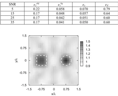
Furthermore, Table IV shows the same quantities for different values of SNR for the case in which εobj = 1.6.
Finally, Figure 2 reports an example of the reconstruction of the relative dielectric permittivity obtained by the proposed
approach in the case in which εobj = 1.6 and SNR = 25 dB.
As can be seen, both cylinders are correctly located. Furthermore, the two cross sections are identified with quite good accuracies.
Table III – Errors on the reconstruction of two cylinders with different cross sections for different values of εobj. SNR = 25 dB.
εobj eεobj eεbg eε eΕ 1.1 0.035 0.009 0.011 0.65 1.2 0.054 0.016 0.019 0.58 1.3 0.079 0.022 0.026 0.56 1.4 0.11 0.028 0.034 0.57 1.5 0.14 0.035 0.043 0.58 1.6 0.17 0.042 0.051 0.60 1.7 0.20 0.049 0.060 0.62 1.8 0.23 0.055 0.068 0.64 1.9 0.26 0.062 0.077 0.67 2.0 0.29 0.068 0.084 0.67
Table IV – Errors on the reconstruction of two cylinders with different cross sections for different values of the signal-to-noise ratio. εobj =
1.6. SNR eεobj eεbg eε eΕ 5 0.22 0.058 0.070 0.79 15 0.17 0.048 0.057 0.64 25 0.17 0.042 0.051 0.60 35 0.17 0.041 0.050 0.60 0.9 1 1.1 1.2 1.3 1.4 1.5 x/λ y/ λ -1.5 -0.75 0 0.75 1.5 -1.5 -0.75 0 0.75 1.5
Figure 2 – Reconstructed distribution of the relative dielectric permittivity. Two cylinders with different shapes. εobj = 1.6. SNR = 25 dB.
In the third example, the considered imaging system is used to reconstruct three separated homogeneous circular cylinders
of radius a = 0.3λ0.
The cylinders are located at
(
0 0)
,) 1
( = 0.75λ ,0.75λ
obj
r robj(2)=
(
−0.75λ0,0.75λ0)
, and , respecti-vely.Moreover, all the cylinders have the same relative dielectric permittivity, i. e., .
(
0 ) 3 ( = 0.,−0.75λ obj r)
obj obj obj obj ε ε ε ε(1) = (2) = (3) =The errors on the reconstructed distribution of the relative dielectric permittivity are shown in Table V for different values
measurement points are also provided.
Table V – Errors on the reconstruction of three circular cylinders for different values of εobj. SNR = 15 dB.
εobj eεobj eεbg eε eΕ 1.1 0.045 0.012 0.015 0.80 1.2 0.064 0.020 0.024 0.67 1.3 0.085 0.026 0.031 0.62 1.4 0.11 0.032 0.039 0.60 1.5 0.13 0.038 0.046 0.59 1.6 0.15 0.043 0.053 0.59 1.7 0.17 0.048 0.060 0.60 1.8 0.20 0.054 0.067 0.62 1.9 0.23 0.059 0.074 0.64 2.0 0.26 0.065 0.082 0.67
As can be seen, the proposed approach is able to yield quite good results for all the considered values of εobj.
Furthermore, Table VI provides the same quantities for different values of SNR in the case in which εobj = 1.4 and the
obtained image for εobj = 1.4 and SNR = 15 dB is reported in Figure 3.
In this image, all the three cylinders are correctly identified, and the predicted values of the relative dielectric permittivity are very close to the exact ones.
Table VI – Errors on the reconstruction of three circular cylinders for different values of the signal-to-noise ratio. εobj = 1.4.
SNR eεobj eεbg eε eΕ 5 0.13 0.047 0.055 0.81 15 0.11 0.032 0.039 0.60 25 0.094 0.027 0.033 0.53 35 0.094 0.026 0.032 0.52 0.8 0.9 1 1.1 1.2 1.3 1.4 1.5 x/λ y/ λ -1.5 -0.75 0 0.75 1.5 -1.5 -0.75 0 0.75 1.5
Figure 3 – Reconstructed distribution of the relative dielectric permittivity. Three circular cylinders. εobj = 1.4. SNR = 15 dB.
V. EXPERIMENTAL RESULTS Finally, the proposed method has been also tested by using experimental data.
The first inverted data have been collected in the anechoic chamber of the Joint Lab. DIBE - EMC S.r.l. (Figure 4). The
object under test is a square dielectric cylinder (side: l = λ0/5; center: (0., 0.); εobj ≈ 2.5), which is enclosed in a square
investigation domain (side: L = λ0/2; number of subdomains: N = 400). The object is illuminated by a transmitting antenna with
a phase center located at (0., 8.4λ0) and working at frequency f = 600 MHz. The scattered electric field is collected by a λ0/4
dipole antenna at M = 41 points located at (in polar coordinates)
rm = (3λ0/5, −7π/6+(m-1)π/30), m=1,…,41. (15)
For this case, a single view has been used. Figure 5 shows the reconstructed distribution of the relative dielectric
Figure 4 – Measurement set up of the anechoic chamber of the Joint Lab DIBE - EMC S.r.l., Genova, Italy. 0.8 0.85 0.9 0.95 1 1.05 1.1 1.15 1.2 1.25 1.3 -0.5 -0.25 0 0.25 0.5 x/λ -0.5 -0.25 0 0.25 0.5 y/ λ
Figure 5 – Reconstructed distribution of the relative dielectric permittivity. Square cylinder. Real data.
The method has also been assessed by inverting data measured in the anechoic chamber of the Fresnel Institue of Marseilles, France, made available by courtesy of prof. K. Belkebir and prof. M. Saillard [13]. The objects under test are two tangent circular homogeneous cylinders. The center of the first one is located at (-0.055, 0.) and its radius is 0.015m. Its relative dielectric permittivity is equal to 3.0, which corresponds to strong scatterer of high contrast with respect to the background. The center of the second one is located at the origin of the frame system and its radius is 0.04m. The relative permittivity of this cylinder is 1.45. The views are 8 and double ridged horn antennas are used as source and receiver.
The v-th view is located at
. ,..., 1 4 ) 1 ( , 67 . 1 v v V v ⎟ = ⎠ ⎞ ⎜ ⎝ ⎛ − = π s (22)
For each view, M = 241 measurement points are used, whose polar coordinates are . ,..., 1 ) 1 ( 3 4 3 ) 1 ( 4 , 67 . 1 m v V M v v m ⎟ = ⎠ ⎞ ⎜ ⎝ ⎛ − + + − = π π π r (23)
The investigation domain is a square with a side of 0.1 m and the electric field is measured at 3GHz.
The scattered-field data have been inverted by using both the second order and the fourth order Born approximation.
Figure 6 reports the obtained results for the cases p = 2 and p = 4. In particular, the figure shows the original and reconstructed dielectric profiles obtained by cutting the objects by (a) the plane y = 0, (b) the plane x = -0.05, and (c) the plane
x = 0.0075.
In both cases, the localization of the objects is very accurate and the permittivity of the larger cylinder is reconstructed very well. Moreover, the fourth order Born approximation allows a better reconstruction of the permittivity of the smaller cylinder with respect to the case p = 2. Anyway, such a permittivity is underestimated because the smaller cylinder is a strong scatterer and the Born approximation do not perform well, as it is well known, in this case.
VI. CONCLUSIONS
In this paper, new results on microwave imaging have been reported. An effective inversion method based on the nonlinear equations of the inverse scattering problem has been proposed and tested.
A regularization scheme constituted by two steps has been successfully applied. Accurate reconstructions, even in noisy environments, have been numerically obtained. Born approximations of several orders have been used and an improvement has been found by using higher order approximations.
Separated dielectric cylinders have been considered and reconstructed under transverse magnetic illumination conditions. A multi-illumination configuration has been applied and the errors on the reconstructed parameters have been carefully evaluated. Moreover, preliminary results concerning the inversion of real scattered-field data, measured inside anechoic chambers, have also been reported.
1 1.5 2 2.5 3 -0.1 -0.05 0 0.05 0.1 εr x [m] Reconstructed values (p=2) Reconstructed values (p=4) Actual values (a) 1 1.5 2 2.5 3 3.5 -0.1 -0.05 0 0.05 0.1 εr y [m] Reconstructed values (p = 2) Reconstructed values (p = 4) Actual values (b)
1 1.5 2 2.5 3 -0.1 -0.05 0 0.05 0.1 εr y [m] Reconstructed values (p=2) Reconstructed values (p=4) Actual values (c)
Figure 6 – Original and reconstructed dielectric profiles with second and fourth order Born approximations. Two contiguous circular cylinders. (a) y = 0, (b) x = -0.05, and (c) x = 0.0075.
APPENDIX
Let be G:X →Y an operator between the Hilbert spaces X and . As it is well known, G is said to be
Fréchet-differentiable at point if there exists a unique linear and continous operator such that, for
Y X x∈ Gx:'X →Y h∈X 0 ' ) ( ) ( lim 0 = − − + → h h G x G h x G x h (A1)
where ⋅ denotes a suitable norm. Gx' is called the Fréchet derivative of F at x. From the equation (A1) it follows that
) ( ' ) ( ) ( 2 h O h G x G h x G + = + x + . (A2)
Equation (A2) allows to obtain the Fréchet derivative of the operator ~(): 2( ) 2( )
obs inv
v
p L L
F Ω → Ω .
Let us start with the case p=1. It results
∫
∫
∫
Ω Ω Ω + + = + + = + inv inv inv d G E h j F d G E h j d G E j h F v inc v v inc v inc v ' ) ' | ( ) ' ( ) ' ( ) ]( [ ~ ' ) ' | ( ) ' ( ) ' ( ' ) ' | ( ) ' ( ) ' ( ) ]( [ ~ ) ( 0 ) ( 1 ) ( 0 ) ( 0 ) ( 1 r r r r r r r r r r r r r r r r r ωμ τ ωμ τ ωμ τ (A3) hence we conclude∫
Ω = inv d G E h j h F v inc v [' ]( ) ( ') ( ') ( | ') ' ~ () 0 ) ( , 1τ r ωμ r r r r r (A4)[
]
∫
∫
∫
∫
Ω − Ω − Ω Ω − + = = + + = = + = = inv inv inv inv d G F j F d G F j d G E j d G F E j F v p v v p v inc v p v inc v p ' ) ' | ( ) ' ]( [ ~ ) ' ( ) ]( [ ~ ' ) ' | ( ) ' ]( [ ~ ) ' ( ' ) ' | ( ) ' ( ) ' ( ' ) ' | ( ) ' ]( [ ~ ) ' ( ) ' ( ) ]( [ ~ ) ( 1 0 ) ( 1 ) ( 1 0 ) ( 0 ) ( 1 ) ( 0 ) ( r r r r r r r r r r r r r r r r r r r r r r r τ τ ωμ τ τ τ ωμ τ ωμ τ τ ωμ τ (A5) Moreover it results[
+]
[
+ +]
= = = +∫
Ω − inv d G h F E h j h F v p v inc v p ' ) ' | ( ) ' ]( [ ~ ) ' ( ) ' ( ) ]( [ ~ ) ( 1 ) ( 0 ) ( r r r r r r r τ τ ωμ τ[
]
[
]
( | ') ' ) ( ) ' ( ~ ) ' ]( [ ~ ) ' ( ) ' ( 2 )' ( , 1 ) ( 1 ) ( 0 r r r r r r r d G h O h F F E h j inv v p v p v inc + + + + + =∫
Ω − − τ τ τ ωμ (A6)Using equation (A5), we obtain
[
]
) ( ' ) ' | ( ) ' ( ] [ ~ ) ' ( ) ]( [ ~ ) ( ' ) ' | ( ) ' ( ] [ ~ ) ' ( ' ) ' | ( ) ' ]( [ ~ ) ' ( ) ]( [ ~ ' ) ' | ( ) ( ) ' ( ] [ ~ ) ' ]( [ ~ ) ' ( ) ' ( 2 )' ( , 1 0 ) ( 2 )' ( , 1 0 ) ( 1 0 ) ( 1 2 )' ( , 1 ) ( 1 ) ( 0 h O d G h F j F h O d G h F j d G F j F d G h O h F F E j inv inv inv inv v p v p v p v p v v p v p v inc + + = = + + + + = = + + + +∫
∫
∫
∫
Ω − Ω − Ω − Ω − − r r r r r r r r r r r r r r r r r r r r r r r r τ τ τ τ ωμ τ τ ωμ τ τ ωμ τ τ τ ωμ (A7)[
]
[
]
) ( ' ) ' | ( ) ' ]( [ ~ ) ' ( ) ]( [ ~ ' ) ' | ( ) ( ) ' ( ] [ ~ ) ' ( ' ) ' | ( ) ' ]( [ ~ ) ' ( ' ) ' | ( ) ' ( ) ' ( ' ) ' | ( ) ( ) ' ( ] [ ~ ) ' ]( [ ~ ) ' ( ) ' ( 2 ) ( 1 0 ) ( 1 2 )' ( , 1 0 ) ( 1 0 ) ( 0 2 )' ( , 1 ) ( 1 ) ( 0 h O d G F h j h F d G h O h F h j d G F h j d G E h j d G h O h F F E h j inv inv inv inv inv v p v v p v p v inc v p v p v inc + + = = + + + + + = = + = + + +∫
∫
∫
∫
∫
Ω − Ω − Ω − Ω Ω − − r r r r r r r r r r r r r r r r r r r r r r r r r r r r τ ωμ ωμ τ ωμ ωμ τ ωμ τ τ (A8)) ( ' ) ' | ( ) ' ( ] [ ~ ) ' ( ' ) ' | ( ) ' ]( [ ~ ) ' ( ) ]( [ ~ ) ]( [ ~ ) ]( [ ~ 2 )' ( , 1 0 ) ( 1 0 ) ( 1 ) ( ) ( h O d G h F j d G F h j h F F h F inv inv v p v p v v p v p + + + + + = = +
∫
∫
Ω − Ω − r r r r r r r r r r r r r τ τ ωμ τ ωμ τ τ (A9) hence we conclude∫
∫
Ω − Ω − + + + = inv inv d G h F j d G F h j h F h F v p v p v v p ' ) ' | ( ) ' ( ] [ ~ ) ' ( ' ) ' | ( ) ' ]( [ ~ ) ' ( ) ]( [ ~ ) ]( [ ~ )' ( , 1 0 ) ( 1 0 ) ( 1 )' ( , r r r r r r r r r r r r τ τ τ ωμ τ ωμ (A10)Equation (A10) along with equation (A4) allows us to compute recursively the Fréchet derivative of the operator ~(v)
p
F for
every value of . p
REFERENCES
[1] G. C. Giakos, "Emerging Imaging Technologies: From Aerospace to Medical Imaging, Bridging the Gap," Proc. IEEE Int. Workshop on Imaging Systems and Techniques, Stresa, Italy, May 14, 2004.
[2] M. Pastorino, "Recent inversion procedures for microwave imaging in biomedical, subsurface detection and nondestructive evaluation," Measurement, Elsevier, special issue on "Imaging Measurement Systems," vol. 36, pp. 257-269, 2004.
[3] Ch. Pichot et al., "Recent nonlinear inversion methods and measurement systems for microwave imaging," Proc. IEEE Int. Workshop on Imaging Systems and Techniques, Stresa, Italy, May 14, 2004.
[4] R. Zoughi, Microwave Nondestructive Testing and Evaluation, Kluwer Academic Publishers, The Netherlands, 2000. [5] S. K. Moore, "Better breast cancer detection," IEEE Spectrum, May issue, 50, 2001.
[6] M. Pastorino, A. Massa, S. Caorsi, "A global optimization technique for microwave nondestructive evaluation," IEEE Trans Instrum. Meas., vol. 51, no. 4, pp. 666-673, Aug. 2002.
[7] P. M. Morse and H. Feshbach, Methods of Theoretical Physics. McGraw-Hill, New York, 1953.
[8] M. Slaney, A. C. Kak, and L. E. Larsen, "Limitation of imaging with first-order diffraction tomography," IEEE Trans. Microwave Theory Tech., vol. 32, pp. 860-873, 1984.
[9] A. Abubakar, P. van den Berg, and S. Semenov, "A robust iterative method for Born inversion," IEEE Trans. Geosci. Remote Sens., vol. 42, pp. 342-354, Feb. 2004.
[10] N. Zaiping and Y. Zhang, "Hybrid Born iterative method in low-frequency inverse scattering problem," IEEE Trans. Geosci. Remote Sens., vol. 36, pp. 749-753, May 1998.
[11] S. Caorsi, A. Costa, and M. Pastorino, "Microwave imaging within the second-order Born approximation: Stochastic optimization by a genetic algorithm," IEEE Trans. Antennas Propagat., vol. 49, no. 1, pp. 22-31, Jan. 2001.
[12] R. Pierri and G. Leone, "Inverse scattering of dielectric cylinders by a second-order Born approximation," IEEE Trans. Geosci. Remote Sens., vol. 37, pp. 374-382, Jan. 1999.
[13] K. Belkebir and M. Saillard, “Special section: Testing inversion algorithms against experimental data,” Inverse Problems, vol. 17, pp. 1611-1622, Nov. 2001.
[14] J. H. Richmond, “Scattering by a dielectric cylinder of arbitrary cross-section shape,” IEEE Trans. Antennas and Propagat., vol. AP-13, pp. 334-341, 1965.
[15] M. Bertero and P. Boccacci, Introduction to Inverse Problems in Imaging, IOP, Bristol, UK, 1998. [16] C. A. Balanis, Advanced Engineering Electromagnetics, John Wiley & Sons, 1989