APPROXIMATE BAYESIAN COMPUTATION FOR COPULA
ESTIMATION
Clara Grazian
Universit´e Dauphine, Paris, France
Dipartimento di Scienze Statistiche, Sapienza Universit`a di Roma, Roma, Italia CREST, Paris, France
Brunero Liseo 1
Dipartimento di metodi e Modelli per l’Economia, il territorio e la Finanza, Sapienza Universit`a di Roma, Roma, Italia
1. Introduction
Copula models are nowadays widely used in multivariate data analysis. Major ar-eas of application include econometrics (Huynh et al., 2015), geophysics (Scholzel and Friederichs, 2008), quantum mechanics (Resconi and Licata, 2015) climate prediction (Schefzik et al., 2013) genetics (He et al., 2012), actuarial science and finance (Cherubini et al. (2004), among the others). A copula is a flexible proba-bilistic tool that allows the researcher to model the joint distribution of a random vector in two separate steps: the marginal distributions and a copula function which captures the dependence structure among the vector components.
From a statistical perspective, whereas it is generally simple to produce reliable estimates of the parameters of the marginal distributions of the data, the problem of estimating the dependence structure, however it is modelled, is crucial and often complex, especially in high dimensional situations. On the other hand, dependence is one of the most fundamental features in (applied) statistics, economics and probability. A huge list of important applications can be found in the recent monograph by Joe (2014).
In a frequentist approach to copula models, there are no broadly satisfactory methods for the joint estimation of marginal and copula parameters. The most popular method is the so called Inference From the Margin (IFM) method, where the parameters of the marginal distributions are estimated first, and then pseudo data are obtained by plugging in the estimates of the marginal parameters. Then inference on the copula parameters is performed using the pseudo-data: this ap-proach obviously does not account for the uncertainty on the estimation of the marginal parameters. Bayesian alternative are not yet fully developed, although
Min and Czado (2010), Craiu and Sabeti (2012), Smith (2013) and Wu et al. (2014) are remarkable exceptions.
In this work we consider the general problem of estimating some specific quan-tities of interest of a generic copula (such as, for example, tail dependence index or Spearman’s ρ) by adopting an approximate Bayesian approach along the lines of Mengersen et al. (2013). In particular, we discuss the use of the BCel algorithm, based on the empirical likelihood approximation of the marginal likelihood of the quantity of interest. Our approach is approximate in two aspects:
i. elicitation of the prior distribution is required only on the quantity of interest. Its prior distribution is combined with the empirical likelihood in order to produce an approximation to the “true” posterior distribution.
ii. we do not use the “true” likelihood function, but rather an approximation based on empirical likelihood theory (Owen, 2010). Hopefully, this will reduce the potential bias for incorrect distributional assumptions.
Note, however, that the word “true” in the above list should be better spelled as “true-under-the-assumed-model”. In situations where a true model is too hard to specify, or too complex to deal with, the empirical likelihood can be an extremely valuable tool.
Our approach can be adapted both to parametric and nonparametric mod-elling of the marginal distributions. The method described in this paper is in the spirit of Hoff (2007), but it is based on a different kind of approximation; the results, although from a different perspective, can be also interpreted in the light of Schennach (2005), where a Bayesian nonparametric interpretation of a tilted version of the empirical likelihood is provided.
2. Preliminaries: Copulae and Empirical Likelihood
A copula model is a way of representing the joint distribution of a random vector X = (X1, . . . , Xm). Given an m-variate cumulative distribution function (CDF)
F , it is possible to show (Sklar, 1959) that there always exists an m-variate
func-tion C : [0, 1]m→ [0, 1], such that F (x
1, . . . , xm) = C(F1(x1), . . . , Fm(xm)), where Fjis the marginal CDF of Xj. In other terms, the copula function C is a CDF with uniform margins on [0, 1]: it binds together the univariate CDF’s F1, F2, . . . , Fmin order to produce the m-variate CDF F . The copula function C does not depend on the marginal distributions of F , but rather it accounts for potential dependence among the components of the random vector X.
For each pair of components of X, say Xi and Xj, let us assume that they have continuous CDF’s Fi and Fj. It is well known that both the transformed variables Ui = Fi(Xi) and Uj = Fj(Xj) have uniform marginal distributions. A semiparametric copula model consists of a parametric model for the joint distri-bution of (Ui, Uj) and no assumptions on the marginal CDF’s. A nonparametric copula is assumed when the joint distribution of (Ui, Uj) depends on an infinite dimensional parameter. In this paper we will allow the marginal distributions Fj’s to follow either a parametric or a non parametric model. For the copula function we will not make any parametric assumption. Rather, we will limit our goal to
the estimation of a particular function of interest of the copula C. A discussion on the classical approaches to semiparametric estimation of copula models can be found in Genest et al. (1995).
Empirical likelihood has been introduced by Owen: Owen (2010) is a com-plete and recent survey; it is a way of producing a nonparametric likelihood for a quantity of interest in an otherwise unspecified statistical model. It is particu-larly useful when a true likelihood is not readily available either because it is too expensive to evaluate or when the model is not completely specified. Assume that our dataset is composed of n independent replicates (x1, . . . , xm) of some random vector X with distribution F and corresponding density f . Rather than defining the usual likelihood function in terms of f , the empirical likelihood is constructed with respect to a given quantity of interest, say φ, expressed as a functional of F , i.e. φ(F ), and then a sort of profile likelihood of φ is computed in a nonparametric way. More precisely, consider a given set of generalized moment conditions of the form
EF(h(X, φ)) = 0, (1)
where h(·) is a known function, and φ is the quantity of interest. The resulting empirical likelihood is defined as
LEL(φ; x) = maxp
n ∏ i=1
pi,
where the maximum is searched over the set of vectors p such that 0 ≤ pi ≤ 1, ∑n i=1pi= 1, and n ∑ i=1 h(xi, φ)pi= 0.
Whereas the first two conditions are obvious and independent of φ, the third one induces a profiling of the information towards the quantity of interest, through a sort of unbiasedness condition.
3. ABC and EL
Approximate Bayesian computation has now become an essential tool for the anal-ysis of complex stochastic models, in the case where the likelihood function is unavailable in closed form or it is too expensive to be repeatedly evaluated (Marin
et al., 2012). It can be considered as a class of popular algorithms that achieves
posterior simulation by avoiding the computation of the likelihood function. A crucial condition for the use of ABC algorithms is that it must be relatively easy to generate new pseudo-observations from the working model, for a fixed value of the parameter vector. In its simplest form, the ABC algorithm “proposes” a (pseudo)-randomly drawn parameter value θ∗ from the prior distribution and a new data set is generated, conditionally on θ∗; then the value is accepted only if the new data are “similar enough” to the actual observed data. It can be proved that the set of accepted values represents a sample from an approximation of the posterior distribution of θ (Sisson and Fan, 2011). However, it is often highly
inefficient to propose values from the prior distribution, since it is generally much more diffuse than the posterior distribution. Many more sophisticated computa-tional strategies are available in order to avoid generating values from the prior distribution, see Marin et al. (2012) for example; here we will not discuss these issues and we rather concentrate on a different ABC approach, which can avoid the most expensive step in computational time, that is the proposal of new data sets. This method has been proposed by Mengersen et al. (2013) and it represents a re-sampling scheme where the proposed values are re-sampled with weights pro-portional to their empirical likelihood. In practice, the algorithm belongs to the family of “sampling importance re-sampling” - SIR, (Rubin, 1988) - methods for models in which the “true likelihood” evaluation is out of reach and the “true” weights are approximated by their empirical likelihood.
for i = 1 to M do repeat
Generate θi from the prior distribution π(θ) Set the weight for θi as ωi= LEL(θi; data). end for
for i = 1 to M do
Draw, with replacement, a value θifrom the previous set of M values using weights ωi, i = 1, . . . , M .
end for
Algorithm 1: BCEL algorithm (Mengersen et al., 2013)
4. The proposed approach
In this paper we propose to adapt the BCELalgorithm of Mengersen et al. (2013) to a situation where the statistical model is only partially specified and the main goal is the estimation of a finite dimensional quantity of interest. In practice this represents the prototypical semiparametric set-up, where one is mainly interested in some meaningful characteristic of the population, although the statistical model may contain nuisance parameters which are often introduced in order to produce more flexible models that might better fit the data at hand. In order to make robust inference on the quantity of interest, a reasonable model should account for the uncertainty on the nuisance parameters, in some way. Even if some of these additional parameters are not particularly important in terms of estimation - they often lack of a precise physical meaning - their estimates can dramatically affect inferences on the parameter of interest. In these circumstances it might be more reasonable and robust to partially specify the model and adopt a semiparametric approach.
Oh and Patton (2013) consider, in a frequentist perspective, a Simulated Method of Moments estimation for copula models. Their paper is very close
in spirit to what we are proposing, although their main goal is the analysis of partially specified models rather than models with an intractable likelihood.
4.1. The algorithm in full detail
We assume that a data set is available in the form of a size n×m matrix X, where
n is the sample size and m is the number of variables, that is
X = x11 x12 . . . x1m x21 x22 . . . x2m . . . . . . xij . . . xn1 xn2 . . . xnm .
In the following, X[·,j] will denote the j-th column (variable) and X[i,·] the i-th row of X, respectively. For each j = 1, . . . , m, we consider the available data information in X[·,j] to produce an estimate of the marginal CDF of X[·,j]. Let
λj = (λ (1) j , λ (2) j , . . . λ (S)
j )′, j = 1, 2, . . . m be the posterior sample obtained from some Bayesian inference method for the distribution of X[·,j]. Notice that the vector λj can be either a sample from the posterior distribution of the parameters of the model we have adopted for X[·,j] or a posterior sample of CDF ’s in a nonparametric set-up. Then we use a copula representation for estimating the multivariate dependence structure of the random vector X,
F (x1, . . . , xm) = Cθ (
F1(x1), F2(x2), . . . , Fm(xm) )
,
where θ is the parameter related to the copula function. Since we are assuming that one has already estimated the marginal Fj(xj)’s, j = 1, . . . , m, one now needs to consider the copula Cθ(·) only. This step can be managed either using some parametric model for the copula (such as Clayton, Gaussian, Skew-t, Gumbel, etc.) or using a nonparametric approach.
Parametric copulae in Bayesian inference have been already investigated in several papers. Here we should mention Hoff (2007), Silva and Lopes (2008), Min and Czado (2010), Smith et al. (2012) and Craiu and Sabeti (2012). In this paper, we take a nonparametric route and we concentrate on some specific function of
Cθ(·), say φ = T (Cθ). This is particularly useful and meaningful in those situations where there is no theoretical or empirical evidence that a given copula should be preferred and we are mainly interested in some specific synthetic measure of the multivariate dependence, like for example, the upper tail dependence index between two components of X, that is
χ = lim u→1P (Uj > u|Uh> u)≈ limu→1 [ 2−log P (Uj< u, Uh< u) log P (Uh< u) ]
where Ui = Fi(xi), i = j, h. Another popular quantity, which we will consider in the final section is the Spearman’s measure of association ρ between two compo-nents of X, say Xh and Xj, which is defined as the correlation coefficient among
the transformed values Ui= Fi(xi), i = j, h or, in a copula language, as ρ = 12 ∫ 1 0 ∫ 1 0 ( C(uj, uh)− uhuj ) dujduh = 12 ∫ 1 0 ∫ 1 0 C(uj, uh)dujduh− 3. (2)
We now describe the algorithm in a pseudo-language:
[1:] For s = 1, . . . , S, use the s-th row of the posterior simulation
λ(s)1 , λ(s)2 , . . . , λ(s)m to create a matrix of uniformly distributed pseudo-data
u(s)= u(s)11 u(s)12 . . . u(s)1m u(s)21 u(s)22 . . . u(s)2m . . . . . . u(s)ij . . . u(s)n1 u(s)n2 . . . u(s)nm with u(s)ij = Fj ( xij; λ (s) j ) .
[2:] Given a prior distribution π(φ) for the quantity of interest φ, for b = 1, . . . , B,
1. draw φ(b)∼ π(φ);
2. compute EL(φ(b); u(s))= ω
bs; s = 1, . . . , S. 3. take the average weight ωb= S−1
∑S s=1ωbs end for
[3:] re-sample - with replacement - from{(φ(b), ω b
)
, b = 1, . . . , B}.
Algorithm 2: ABCOP algorithm
The final output of the above algorithm is then a posterior sample drawn from an approximation of the posterior distribution of the quantity of interest φ. There are several critical issues both in the practical implementation of the method and in its theoretical properties. First, the empirical likelihood is based on moment conditions of the form (1). In practical applications these conditions might hold only asymptotically. This is the case, for example, of the Spearman’s ρ, which we discuss in the next session. Its sample counterpart ρn is only an asymptotically unbiased estimator of ρ so the moment condition is strictly valid only for large samples. Also, prior information is only provided for the marginal distributions and for φ: this, of course, has advantages and, on the other hand, poses the-oretical issues. The main advantage is the ease of elicitation: one need not to elicit unnecessary aspects of the prior distribution. This is mainly in the spirit of the partially specified models, quite popular in the econometric literature. An-other obvious advantage of the proposed approach is the implied robustness of
the method, with respect to different prior opinions about non-essential aspects of the dependence structure. The most important disadvantage of the method is its inefficiency when compared to a parametric copula, under the assumption that the parametric copula is the true model. The practical implementation of the algorithm is quite simple in R ; it use some functions contained in the suite gmm: see for example Chauss´e (2010).
From a computational perspective the above algorithm is quite demanding, since one needs to run a BCELalgorithm for each row of the posterior sample from the marginals. Even though the estimation of the marginal densities of the X[·,j]’s might not require a huge values of iterations S, still it might be very expensive to run S different BCEL algorithms. To avoid this computational burden, we propose to modify the above algorithm by simply performing a single run of the
BCEL algorithm, where, for each iteration b = 1, . . . , B, a randomly selected (among the S rows) row λsis used to transform the actual data into pseudo-data lying in [0, 1]m. With this modification the above algorithm gets transformed into Algorithm 3.
5. A simple illustration: Spearman’s ρ
We first illustrate the method in a simple situation, with m = 2, and assuming that the two marginal distributions of the data are known: without loss of generality we can then assume that they are both uniform in [0, 1]; in this case there are no practical differences between Algorithm 2 and Algorithm 3.
The Spearman’s ρ measure of dependence has been defined in (2). Starting from a sample of size n from a bivariate distribution, say (xi, yi), i = 1, . . . , n, the sampling counterpart of ρ, say ρn, is nothing but the correlation among ranks and it can be written as ρn= 1 n n ∑ i=1 ( 12 n2− 1RiSi− 3 n + 1 n− 1 ) , (3) where Ri= rank(xi) = n ∑ k=1 I(xk≤ xi), Si= rank(yi) = n ∑ k=1 I(yk ≤ yi), i = 1, . . . , n.
Since we assume that the marginal distributions are known, pseudo-data coincide with the actual data, and we work with a single n× 2 matrix U whose generic element is given by uij = xij with uij ∈ [0, 1], i = 1, . . . , n, j = 1, 2. Then we take the ranks (Ri, Si) of the original values and compute ρn. Also we are able to evaluate the empirical likelihood of ρ for a given value of ρnas maxpiEL(ρ; ρn) = ∏n
i=1npi(ρ) under the constraints ∑n i=1pi= 1, 0≤ pi≤ 1, i = 1, . . . , n and n ∑ i=1 pi (12RiSi n2− 1 − 3 n + 1 n− 1 − ρ ) = 0.
[1:] For j = 1, . . . , m, produce a posterior sample for the parameters of the marginal distributions of the X[·,j]’s, say λj= λ
(1) j , λ (2) j , . . . , λ (S) j , j = 1, . . . , m. Store them into a S× k matrix λ = (λ1, . . . , λj, . . . , λm) where k is the sum of the dimensions of the parameter spaces of the marginal distributions.
[2:] Given a prior distribution π(φ) for the quantity of interest φ, for b = 1, . . . , B,
1. draw a random uniform integer t(b) in{1, 2, . . . , S}.
2. use the t(b)-th row of λ to create a matrix of uniformly distributed
pseudo-data u(t(b))= u(t(b))11 u(t(b))12 . . . u(t(b))1m u(t(b))21 u(t(b))22 . . . u(t(b))2m . . . . . . u(t(b))ij . . . u(t(b))n1 u(t(b))n2 . . . u(t(b))nm with u(t(b))ij = Fj ( xij; λ (t(b)) j ) . 3. draw φ(b)∼ π(φ); 4. compute EL ( φ(b); u(t(b)) ) = ωb; end for
[3.] store the values(φ(b), ω b
)
, b = 1, . . . , B.
[4.] re-sample - with replacement - from{(φ(b), ω b
)
, b = 1, . . . , B}.
Algorithm 3: Modified ABCOP algorithm
From general results on empirical likelihood (Owen, 2010), one has
EL(ρ; ρn) = n ∏ i=1 ( 1 + ηg(Ri, Si; ρ) )−1
where η is the Lagrange multiplier which can be explicitly obtained from n ∑ i=1 g(Ri, Si; ρ) 1 + ηg(Ri, Si; ρ) = 0, where g(Ri, Si; ρ) = 12RiSi n2− 1 − 3 n + 1 n− 1− ρ.
We can then use Algorithm 2, with S = 1, to produce a posterior sample for the quantity of interest ρ.
5.1. A small scale simulation
As an illustration we have simulated 1, 000 samples of size n = 100 from a bivariate Clayton’s Copula, whose expression is
C(u, v) =
{
uv θ = 0
(
u−θ+ v−θ− 1)−1/θ θ > 0.
For comparative purposes we have also implemented the nonparametric frequentist procedure described in Genest and Favre (2007), where a confidence interval for the Spearman’s ρ is constructed based on the asymptotic sampling distribution of
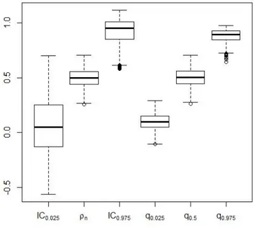
ρn. In the simulation θ has been set equal to 1.076, which implies ρ≈ 0.5. Figure 1 compares the frequentist behavior of confidence procedure and our proposal. The first three box-plots show the sampling (over the 1, 000 generated samples) distribution of i) the lower limit of the equal-tail confidence interval with nominal coverage set at 0.95, ii) the point estimate ρn, and iii) the upper limit of the equal-tail confidence interval with nominal coverage set at 0.95. The last three box-plots show the sampling distribution of some specific quantiles (namely the 2.5th, the median and the 97.5th percentiles) of the approximated posterior distribution. Samples were generated by fixing θ = 1.076. The prior distribution for ρ has been taken Unif(−1, 1). Computations were done in R , using libraries copula and gmm. One can see that our procedure produces more precise estimates in terms of intervals. The empirical estimate and the posterior median behave very similarly. The average length of the confidence interval is 0.820 while the average length of the equal-tail 0.95 credible set is 0.784 In 626 out of 1, 000 simulation, the Approximate Bayesian interval was shorter than the classical confidence interval.
5.2. Simulated non uniform data
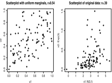
Here we show an example of bivariate data with non uniform marginal distribution. Data were generated from a Clayton copula with θ = 1.076 (ρ ≈ 0.5), and the two marginal distributions were transformed into an exponential distribution with mean 1/3 (for X1) and a Gaussian distribution with mean 3 and variance 1 (for
X2). Figure 2 shows the scatterplot of raw and transformed data. In this particular case the observed value for ρn was 0.568.
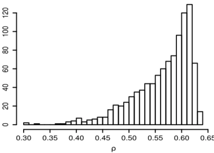
Figure 3 shows the histogram of the BCEL posterior sample for ρ obtained from Algorithm 2. One can notice that the posterior mass is practically entirely on the right of zero, and the posterior mean is 0.56, very close to the observed ρn.
5.3. An alternative estimator
From a purely pragmatic perspective, it might be tempting to follow an uncon-ventional and “hybrid” route, which we now describe. For each s = 1, . . . , S, 1. Provide an estimate of φ, using ˆφ(s)from the plugged-in model
Figure 1 – 1, 000 simulations from a Clayton copula: sample size is 100; the true value of ρ is equal to 0.5. The six box-plots respectively shows the simulated sampling distribution of: i) the lower limit of the equal-tail confidence interval with nominal coverage set at 0.95, ii) the point estimate ρn, iii) the upper limit of the equal-tail confidence interval
with nominal coverage set at 0.95. iv) the 2.5-th v) the 50-th and vi) the 95-th quantile of the approximate posterior distribution.
0.0 0.2 0.4 0.6 0.8 1.0 0.0 0.2 0.4 0.6 0.8 1.0
Scatterplot with uniform marginals, r=0.54
u1 u2 0 1 2 3 4 5 0.0 0.5 1.0 1.5
Scatterplot of original data: r=.39
x1: N(3,1)
x2: Exp(3)
Figure 2 – Scatterplot of the simulated data and pseudo-data: X1 ∼ Exp(3); X2 ∼
N (3, 1)
BCel Posterior distribution of rho
ρ −0.2 0.0 0.2 0.4 0.6 0.8 1.0 0.0 0.5 1.0 1.5
In particular, one could use a sort of maximum likelihood estimate of φ, as-suming that the sampling distribution is given by (4).
2. Use the distribution of the ˆφ(s)’s as a surrogate of the posterior distribution of
φ.
This approach is a further approximation in many ways. First, the distribution of ˆφ(s)’s in step 2 of the above procedure could not properly be treated as a posterior distribution, since we have not introduced any prior distribution on φ. Second, the distribution in step 2 is not a distribution on φ: rather, it can be interpreted as the posterior distribution of the following quantity
ˆ
φ(Λ) = argmaxφp (x| marginals, φ, Λ) . (5)
Notice that
EΛ( ˆφ(Λ)) ̸= argmaxφEΛ(p(x| marginals, φ, Λ) = argmaxφIL(φ; x) = ˆφ(IL),
where the above expectation is taken with respect to the posterior distribution of the marginal parameters Λ, based on the “marginal” samples and suitable prior information, and IL represents the “correct” integrated likelihood,
IL(φ; x) =
∫ Λ
p(x; λ, φ)π(λ|φ)dλ.
Also, Var ( ˆφ(Λ)) under-reports the variability of the estimator, since M SE = Var ( ˆφ(Λ)) +(EΛ( ˆφ(Λ))− ˆφ(IL))2
However, in practical applications this method works better than the IFM ap-proach, described in§1. Figure 4 shows the behavior of this method with the data used in Figure 2. One can notice a slight bias towards larger values of ρ and an incorrect report of uncertainty.
6. Example: Spearman’s ρ for Student-t log-returns
We now analyze a real data-set containing the log-returns FTSE-MIB of two Italian banks, Monte dei Paschi di Siena (BMPS) and Banco Popolare (BP), by assuming that the log-returns for each bank may be described by a GARCH(1,1) model with Student-t innovations for the log-returns {yt} from 01/07/2013 to 30/06/2014 (only weekdays) available on the web page https://it.finance.yahoo.com.
The GARCH(1,1) model for Student-t innovation may be rewritten via data augmentation, following Geweke (1993):
Hybrid estimation: pseudo ML distribution ρ 0.30 0.35 0.40 0.45 0.50 0.55 0.60 0.65 0 20 40 60 80 100 120
Figure 4 – Hybrid method: “posterior” distribution of ˆφ(λ)
yt= εt √ ν− 2 ν ωtht t = 1,· · · , T εt∼ N (0, 1) ωt∼ IG (ν 2, ν 2 ) ht= α0+ α1y2t−1+ βht−1 t = 1,· · · , T
where α0 > 0, α1, β >= 0 and ν > 2, N (0, 1) denotes the standard normal distribution and IG(a, b) denotes the inverted gamma distribution with shape pa-rameter a and scale papa-rameter b. Figure 5 shows the scatterplot of the log-returns and the transformed version of them, using, as a point estimate, the posterior mean of each parameter.
For each bank, the posterior distribution of the model parameters (α0, α1, β, ν) may be approximated by using the R package bayesGARCH (Ardia and Hooger-heide, 2010). Once a sample from the approximated distribution is simulated for each parameter and for each bank, Algorithm 3 is applied as follows:
for m = 1,· · · , M
1: Simulate a value ρ(m)∼ Unif(−1, 1).
2: Sample two integer values b(m)j (j = 1, 2) in {1, · · · , S}, where S is the number of posterior simulations.
3: Consider the b(m)j -th row of the MCMC output for the parameters of the
Figure 5 – Scatterplot of the log-returns of the investments of Monte dei Paschi di Siena (BMPS) and Banco Popolare (BP) on the left and of the transformed data on the right.
Figure 6 – Approximation of the posterior distribution of the Spearman’s ρ for the log-returns of the investments of two Italian institutes based on 10, 000 simulations.
4: Compute pseudo-data u(m)ij for i = 1,· · · , T and j = 1, 2 as u(m)ij = Fνj ( yi; νj(m)− 2 νj(m) h(m)ij )
where Fν(x, d) is the CDF of a Student-t distribution with ν degrees of freedom and scale parameter d.
5: Compute the estimated sample Spearman’s ρ(m)n as in (3) and the weight relative to the simulated ρ(m) as ω(m) = EL(ρ(m)
n ; u (m) 1 , u (m) 2 ) as in Owen (2010).
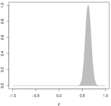
The output of Algorithm 3 relative to the log-returns of Monte dei Paschi di Siena and Banco Popolare are shown in Figure 6: the estimated posterior mean of ρ is 0.614.
Acknowledgements
The Authors are grateful to two anonymous referees for their helpful sugges-tions and to N. Lunardon for providing some R funcsugges-tions, very useful for our simulation. C. Grazian’s research has been sponsored by Universit`a ItaloFrancese (Universit´e FrancoItalienne). B. Liseo’s research has been sponsored by grant n. C26A13BBCB, Sapienza Universit`a di Roma, 2013.
References
D. Ardia, L. Hoogerheide (2010). Bayesian Estimation of the GARCH(1,1)
Model with Student-t Innovations. The R Journal, 2, no. 2, pp. 41–47.
P. Chauss´e (2010). Computing Generalized Method of Moments and Generalized
Empirical Likelihood with R. Journal of Statistical Software, 11, no. 34, pp.
1–35.
U. Cherubini, E. Luciano, W. Vecchiato (2004). Copula Methods in Finance. John Wiley & Sons, New York, San Francisco, Calif.
V. R. Craiu, A. Sabeti (2012). In mixed company: Bayesian inference for
bivariate conditional copula models with discrete and continuous outcomes. J.
Multivariate Anal., 110, pp. 106–120.
C. Genest, A.-C. Favre (2007). Everything you always wanted to know about
copula modeling but were afraid to ask. Journal of Hydrologic Engineering, pp.
347–368.
C. Genest, K. Ghoudi, L. Rivest (1995). A semiparametric estimation
procedure of dependence parameters in multivariate families of distributions.
J. Geweke (1993). Bayesian treatment of the independent Student-t linear model. J. Appl. Econometr., S1, no. 8, pp. S19–S40.
J. He, H. Li, A. C. Edmondson, D. L. Rader, M. Li (2012). A Gaussian
copula approach for the analysis of secondary phenotypes in casecontrol genetic association studies. Biostat., 13, no. 3, pp. 497–508.
P. Hoff (2007). Extending the rank likelihood for semiparametric copula
estima-tion. The Annals of Applied Statistics, 1, no. 1, pp. 265–283.
V. N. Huynh, V. Kreinovich, S. Sriboonchitta (2015). Modeling Dependence
in Econometrics . Springer, New York.
H. Joe (2014). Dependence modelling with copulas, Monographs on Statistics and
Applied Probability, 134. Chapman & Hall–CRC Press, London.
J. Marin, P. Pudlo, C. Robert, R. Ryder (2012). Approximate Bayesian
computational methods. Statistics and Computing, 6, no. 22, pp. 1167–1180.
K. Mengersen, P. Pudlo, C. Robert (2013). Bayesian computation via
em-pirical likelihood. Proc. of the National Academy of Sciences, 4, no. 110, pp.
1321–1326.
A. Min, C. Czado (2010). Bayesian Inference for Multivariate Copulas using
Pair- copula Constructions. Journal of Financial Econometrics, 4, no. 8, pp.
511–546.
D. Oh, A. Patton (2013). Simulated Method of Moments Estimation for
Copula-Based Multivariate Models. J. Amer. Stat. Assoc., 502, no. 108, pp. 689–700.
A. Owen (2010). Empirical Likelihood. Chapman & Hall/CRC Press, New York (USA).
G. Resconi, I. Licata (2015). Entropy and Copula Theory in Quantum
Mechan-ics. In Proceedings of the 1st Int. Electron. Conf. Entropy Appl., 3–21 November 2014, Sciforum Electronic Conference Series.
D. Rubin (1988). Using the SIR algorithm to simulate posterior distributions (with
discusion). In Bayesian Statistics 3 J.M. Bernardo, M.H. DeGroot, D.V. Lind-ley, and A.F.M. Smith, Eds., Oxford University Press, Oxford (UK), Bayesian
Statistics, pp. 395–402.
R. Schefzik, T. L. Thorarinsdottir, T. Gneiting (2013). Uncertainty
Quantification in Complex Simulation Models Using Ensemble Copula Coupling.
Statist. Sci., 28, no. 4, pp. 616–640.
S. Schennach (2005). Bayesian exponentially tilted empirical likelihood. Biometrika, 1, no. 92, pp. 31–46.
C. Scholzel, P. Friederichs (2008). Multivariate non-normally distributed
random variables in climate research: introduction to the copula approach.
R. d. S. Silva, H. F. Lopes (2008). Copula, marginal distributions and model
selection: a Bayesian note. Stat. Comput., 18, no. 3, pp. 313–320.
S. Sisson, Y. Fan (2011). Likelihood-free MCMC. In Handbook of Markov chain
Monte Carlo, Chapman & Hall/CRC, London, Handb. Mod. Stat. Methods, pp.
313–335.
M. Sklar (1959). Fonctions de r´epartition `a n dimensions et leurs marges. Publ.
Inst. Statist. Univ. Paris, 8, pp. 229–231.
M. Smith (2013). Bayesian Approaches to Copula Modelling. In Hierarchical
Models and MCMC: A Tribute to Adrian Smith, P. Damien, P. Dellaportas, N. Polson, and D. Stephens (Eds), Oxford University Press, Oxford (UK), Bayesian
Statistics, pp. 395–402.
M. Smith, Q. Gan, R. Kohn (2012). Modelling dependence using skew-t copulas:
Bayesian inference and applications. Journal of Applied Econometrics, 3, no. 27,
pp. 500–522.
J. Wu, X. Wang, S. Walker (2014). Bayesian Nonparametric Inference for a
Multivariate Copula Function. Methodol. Comput. Appl. Probab., 1, no. 16,
pp. 747–763.
Summary
We describe a simple method for making inference on a functional of a multivariate distri-bution. The method is based on a copula representation of the multivariate distribution and it is based on the properties of an Approximate Bayesian Monte Carlo algorithm, where the proposed values of the functional of interest are weighed in terms of their em-pirical likelihood. This method is particularly useful when the “true” likelihood function associated with the working model is too costly to evaluate or when the working model is only partially specified.