Variational problems in transport theory with mass concentration

(1)

Scuola Normale Superiore

Pisa

Corso di Perfezionamento in Matematica

Triennio 2004–2006

Variational problems

in transport theory

with mass concentration

Candidato Relatore

(2)

(3)

Introduction

In this thesis we analyze several problems from the calculus of variations in the framework of optimal transport theory. We are mainly concerned with optimization problems from this theory and with other transportation prob-lem which are alternative to the classical Monge-Kantorovich formalization. Most of the models we present come from application purposes and the set of possible applications includes urban economics, biology, fluid mechanics and geophysics.

The main topic of the thesis consists of the study optimal transport problem where some kind of concentration phenomena occur: on the one hand concentration of the marginal measures and on the other concentration along the transport itself.

The first subject, concentration of marginal measures, has been devel-oped in the form of Transport and Concentration Problems, i.e. minimization problems where the unknowns are probability measures and the quantity to be minimized involves some functional encouraging or discouraging their concentration or dispersion and some transport costs as well. In particular, in these problems, transport appear only through their minimal value and we are in general not interested in finding the variables (transport plans, maps. . . ) that actually realize the minimum, and we are only concerned with the properties of “optimal” marginal measures. These problems have some quite natural interpretation from a modelistic point of view. For in-stance, if we are concerned with the planning of a geographical region, we may be interested in finding a concentrated distribution of production cen-ters together with a spread distribution of consumers, keeping anyway as small as possible the transportation costs for commuting or bringing the product to the consumers. Similar problems may also have an interpreta-tion in the study of the shape of certain biological objects, such as leaves; these are in fact objects whose goal is to maximize their extension to take advantage of sunlight, but they receive their nutrient from a single concen-trated source and the transport cost for this nutrient is to be taken into

(7)

account.

The attention that we give to these problems dates back to the Laurea Thesis [66], prepared in 2003 under the direction of Prof. Buttazzo, and has evolved in the years, considering several models and discussing the corre-sponding results. A detailed report on these models is exactly the aim of the first part of this thesis. Our attention will be devoted to some modeling aspects and to the analysis of optimality conditions. In particular necessary optimality conditions, typically of the first order, are a key feature of this thesis. They are exploited as much as possible to obtain regularity, qualita-tive properties and, when possible, explicit expressions for the minimizers. In this case, as the unknowns are measures and hence belong to a nice vector space, differentiation is often feasible and this program gives unexpectedly strong results.

The second of the subjects we mentioned, concentration along transport, has a more classical structure: we are given the starting and arrival measures and we look for the optimal structure which transports the first onto the second. What is important is that in some applications we want to take into account how much the transportation appears to be concentrated: for instance if too many people pass through a same road in a city there could be a congestion effect; on the other hand if we need to create a road system, we would like to concentrate most of the path that different drivers follow on a same road, so that we only need to build few larger roads instead of several smaller ones. This suggests that there should be some quantities measuring how much the transportation is concentrated and, according to the different applications, we would like to consider minimization problem which encourage or discourage this concentration. It seems reasonable to consider Monge’s problem as the concentration-neutral one and that we may create variants departing from this one.

In the thesis the main model discouraging concentration of transport, i.e. taking into account congestion effects, is hidden in Chapter 2, in the middle of Transport and Concentration Problems. In such a chapter we only briefly present it and we are much more interested in its minimal value, in the sense that we will use it as a functional of the marginal measures. A more refined and self-contained study of congestion models is in progress in [36] but it has not been included in this thesis due to its preliminary state. On the other hand a lot of attention is given to transport problems encouraging joint transportation. There is a wide literature on them, as they are very natural in applications, and they give raise to some optimal one-dimensional branching structures. these structures are dealt with in the thesis in three chapters (6,7 and 9), together with a brief review of the

(8)

already existing results.

Let us see now how the themes above have been developed in the chapters of the thesis. Each chapter corresponds roughly to a paper that has been prepared during this three-years doctoral period: some of these articles have been published and some are accepted. Only the last chapter contains some new computations not yet presented in preprint form.

Chapters 1, 2 and 3 are the first part of the thesis and present trans-port and concentration problems. In these chapters we are concerned with optimization problems of the following kind:

min

µ,ν∈P(Ω)F(µ, ν) := T (µ, ν) + F (µ) + G(ν),

where the functional T represents transport costs between the two proba-bility measures µ and ν and F and G are functionals over the space _P(Ω) of probability measures on Ω with opposite behavior: the first favors spread measures and penalizes concentration while the latter, on the other hand, favors concentrated measures. Chapter 1 is devoted to a problem fitting into this framework that has been proposed in the Laurea Thesis [66] and then in [28]. A particular choice of the functionals T, F and G is performed: we set T (µ, ν) = W_pp(µ, ν), F (µ) = (R Ωf (u) dLd if µ = u· Ld +_∞ otherwise, G(ν) = (_P k∈Ng(ak) ifν =Pk∈Nakδxk +_∞ otherwise.

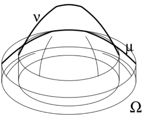
The functions f and g must obviously satisfy some conditions, and in partic-ular f must be convex and g subadditive. In this way T is the minimum of a Kantorovich optimal transport problem and F and G are local semicontinu-ous functionals over measures (see [16], [17] and [18]). A short introduction of this useful class of functionals over measures has been inserted into the chapter: in this way we can see that both concentration preferring func-tionals (as G is) and funcfunc-tionals favoring spread measures (as F does) fall into this class. Some emphasis is given throughout the Chapter to the in-terpretation of such a variational model in terms of urban planning: here the measure µ represents residents’ distribution in the urban area Ω and ν stands for the distributions of services. The first measure has to be as spread as possible to maximize the average use of land of the citizens, while

(9)

the second has to be concentrated in order to increase the efficiency f the production (i.e. we have positive externalities for nearby services). How-ever, the commuting transportation cost for people needing to move from home to services must be considered as well. From the interpretation of the model the convexity and subadditivity assumptions on f and g, which are useful for technical reasons, turn out to be quite natural.

Besides the modelistic side, the chapter is devoted to some mathematical aspects of the problem. In this minimization existence results are straight-forward, at least when Ω is compact. This is due to the semicontinuity of the functionals with respect to weak convergence of measures. Our atten-tion is consequently mainly devoted to optimality condiatten-tions. Notice that any pair (µ, ν) giving finite value to F must be necessarily composed by an absolutely continuous measure µ with density u _{∈ L}1(Ω) and by a purely atomic measure ν. Hence it is interesting to deduce properties on the density u and on the location of the atoms of ν. The main results are obtained by perturbing an optimal µ into a new measure µ+ε(µ1−µ) and keeping frozen

ν. The duality formula in mass transportation plays a crucial role. The idea is very simple and the computations are simple as well, up to overcoming some technical difficulties about Kantorovich potentials. The result we get is the following: if u is the density of µ and ψ a suitably chosen Kantorovich potential between µ and ν we have

f0(u) + ψ = const a.e.

For this result two proofs are provided. The second, mainly based on convex analysis, has been suggested by an anonymous referee while reviewing the ar-ticle [28]. In the original paper, anyway, such a proof was only sketched and it actually requires some preliminary work before being performed. Then, after understanding optimality conditions for fixed ν the attention comes back to the whole problem when both µ and ν vary and the results are applied in order to characterize the global optima. The same results are also useful to gain some compactness when the problem is posed in an un-bounded domain, such as Ω = Rd, where the existence is no longer trivial. The qualitative shape of the optimal configurations is in the end the follow-ing: ν is composed by finitely many atoms xi and µ = u· Ldis concentrated

on some balls Bi centered at these atoms, with radially decreasing densities

given by an explicit formula:

u = (f0)−1(ci− |x − xi|p) for x∈ Bi.

These balls may be interpreted as subcities (or cities if Ω is thought of as a larger region) and the atoms are their centers, where services are located.

(10)

In Chapter 2 we introduce in the subject of urban planning the concept of traffic congestion. The source of inspiration is a set of works by Beckmann ([10] and [11]) and the idea is the following: it is well known that the Monge-Kantorovich problem for a distance cost_{|x − y| is equivalent to the minimal} flow problem inf ½Z Ω|Y (x)|dx : ∇ · Y = µ − ν in Ω, Y · n = 0 on ∂Ω ¾ ;

if one instead looks at the problem

inf ½Z

Ω|Y (x)|

2_{dx :} _{∇ · Y = µ − ν in Ω, Y · n = 0 on ∂Ω}

¾

we are not only minimizing the total movement that is necessary to pass from µ to ν, but we are also penalizing an excessive concentration of this movement. At the beginning of the chapter this congestion model for opti-mal transportation is explained in more details. In minimizing the L2 norm of the vector field Y under divergence constraints an elliptic equation with Neumann boundary conditions appears as an Euler equation. the optimal flow Y is in fact characterized by

Y =∇φ; (

−∆φ = µ − ν in Ω,

∂φ

∂n = 0 on ∂Ω,

where the equation as to be taken in the weak sense.

Anyway, as we said above, in the chapter we are not much interested in the minimization problem itself and in understanding how the optimal flow looks like, but we are more interested in using the minimal L2 norm of the flow as a quantity which represents the congestioned transport cost between the two measures. Then we insert this quantity in a Transport and Concentration Problem as in Chapter 1. It is quite easy to convince oneself, due to the link with elliptic theory, that the infimum of the L2_{− flow is} infinite if µ_{− ν does not belong to a suitable functional space. This requires} a sort of H−1 regularity and in particular prevents ν from having atoms. Hence, in the functional F we will not only replace T by a congestion term, but G has to be replaced too, as the atomic choice of Chapter 1 is no longer possible. A very natural choice for the functional G is the following one, that we call interaction energy, and it is well known in the framework of optimal transport from the work of McCann ([58]):

G(ν) = Z

Ω×Ω

(11)

where V (x, y) is, for instance, an increasing function of the distance between x and y. The idea is to take the interaction cost for a service located at x and another service located at y and average it with respect to the distribution of services. For the functional F we keep the same choice as in Chapter 1 but we particularize it to the case f (s) = s2_{, and in the end we get the}

following functional

F(µ, ν) =_{||µ − ν||}2_X0+||µ||2_L2 + G(ν),

which is a quadratic functional. Here the space X0 is the dual space of X = {ψ ∈ H1(Ω) : R

Ωψ = 0} with norm ||ψ||X = ||∇ψ||L2 (this representation

of the congestion cost of transport comes from the representation formula for the optimal flow Y ).

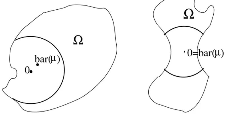
After setting the problem and getting some existence results, as in Chap-ter 1 we look for optimality conditions. Here too the first step is freezing ν and getting a convex quadratic problem in µ. Then the attention goes to the problem in ν only. This is more involved than what we had in Chapter 1 since now ν is no longer discrete and it can a priori be any probability mea-sure since G(ν) <_{∞ for any ν ∈ P(Ω). We prove consequently a regularity} result for ν which guarantees that ν is actually absolutely continuous with bounded density under certain assumptions (in particular, we need Ω to be convex: in the non-convex case ν may have a singular part concentrated on the non-convex part of ∂Ω). The result is obtained by approximation and it is interesting to see that a very powerful regularization technique comes actually from the use of Monge-Kantorovich theory. In fact the original idea was to perturb the problem by adding a small term ε||ν||2

L2 in order

to force the optimal νε to have a density and then to get uniform estimates

on the L∞ _{norm of ν}

ε. Unfortunately, in this way we could retrieve at the

limit some information only on a particular minimizer of F, i.e. the one which is approximated by minimizers of the perturbed problems. As we are not facing a convex problem we have no guarantee that there is a unique minimizer and we would like to have a regularity result which is valid for arbitrary minimizers. To do this we decide to add a small perturbation of the kind εW2

2(ν, ν), where ν is a minimizer that we can fix. In this way

we are somehow forcing the minimizers νε to converge to ν. What is

inter-esting is that, in computing optimality conditions for the minimizers of the perturbed problems, the Kantorovich potential, induced by the presence of the Wasserstein distance W2, appears. Then, well-known estimates on

Kan-torovich potentials help in getting uniform bounds on the densities of νε.

After a long part devoted to regularity the chapter contains some explicit examples. The one-dimensional case is treated in detail and in this case it

(12)

turns out that the functionals involved have some displacement convexity properties (and the proof of this fact is interesting in itself). Then, the two-dimensional radial case is treated under some assumptions that ensure the uniqueness (and hence the radiality) of the solution. The case of a ball, of the whole space and of a crown is treated with explicit solutions. The whole work in Chapter 2 comes from a joint paper with Guillaume Carlier ([37]) that has been developed during a three months visit at the University of Bordeaux IV in 2004.

Chapter 3 contains a subsequent short work ([67]) that has been written to complete the subject of Transport and Concentration Problems. The goal was twofold: first, presenting this class of problems as a whole subject, with possible applications in urban planning (but not only); then, completing the framework of the problems we studied. In fact with G. Buttazzo we studied the problem where the transport cost was given by a Wasserstein distance and the concentration one by a local functional on atomic measures and with G. Carlier the case of a congestion transport cost and an interaction concentration cost. We already noticed that the case of congestion + local atomic functionals is not meaningful as it would have lead to a constantly infinite functional. Consequently, to complete the framework it is interesting to consider the Wasserstein + interaction case. The problem is hence the minimization of the functional

F(µ, ν) = W₂2(µ, ν) + F (µ) + Z

Ω×Ω

V (x, y)(ν⊗ ν)(dx, dy),

where F is the same as in Chapter 1. In Chapter 3 the goals are: determining some optimality conditions (mainly on ν for fixed µ, because those on µ for fixed ν come directly from what we saw in Chapter 1), using them to get L∞ regularity, analyzing an explicit, quadratic, example. The regularity is obtained by the same scheme as in Chapter 2: almost the same kind of perturbations are performed, but the results on elliptic PDEs are here replaced by some results on Monge-Amp`ere equation. This comes from the fact that the Kantorovich potential plays here the role that in the previous case was played by the solution of the elliptic PDE. A more refined analysis of the behavior of the Kantorovich potential on the boundary of Ω allows to give a result under milder assumptions than what we did in Chapter 2. Anyway, at least a third of the Chapter is devoted to the general topic of transport and concentration problems, and a general definition of concentration preferring functional is given: a functional G : _{P(Ω) → R ∪ {+∞} is said to be} concentration preferring if we have G(t]ν) ≤ G(ν) for any ν ∈ P(Ω) and

(13)

well-known variational problems fall into this class of problems. This is the case for instance of optimal location problems, which are quite studied in urban economics, but also of other average distance problems that will be discussed in Chapter 8 as well.

From Chapter 4 on our attention begins to be more directed towards branched transport problems. These problems are quite natural when we look at situations where we want to encourage joint transportation, for in-stance because building a network system with few large roads is cheaper than building several small roads. The structures that arise are all charac-terized by a first gathering of the masses, followed by joint transportation paths and finally a branching distribution towards the individual destina-tions. These structures and these problems are likely to appear also in natural phenomena, for instance in leaves, trees, river basins and blood ves-sels, and not only in human-built systems. The first mathematical precise formulation of the problem is due to Gilbert, who looked at it, in its discrete version, from the point of view of the applications in communication net-works (see [48]). Once given some sources xi with masses ai and some sinks

yj wth masses bj, his model consists in solving the following minimization

problem

min E(G) := X

h

w_hαH1(eh),

where the infimum is among all weighted oriented graphs G = (eh, ˆeh, wh)h

which fulfill the Kirchoff law at any vertex (at any xi we have ai+ incoming

mass = outcoming mass, at any yj we have incoming mass = outcoming

mass +bj and at all the other vertices incoming and outcoming mass are

equal). The exponent α is a fixed parameter 0 < α < 1 so that the function t_{7→ t}α _{is concave and subadditive.}

The main recent mathematical interest on this subject has been try-ing to generalize this problem to the case of non-discrete measures µ and ν. There are very interesting models by Qinglan Xia ([72]), Maddalena-Solimini-Morel ([57]) and Bernot-Caselles-Morel ([13]). Chapter 4 contains a different approach that we tried to give to the problem in a joint work with Alessio Brancolini and Giuseppe Buttazzo. The main idea is looking at an interpolation between µ and ν, i.e a curve γ in the space of probability measures, which minimizes a certain length functional

J (γ) = Z 1

0

J(γ(t))|γ0|(t) dt,

where J : _{P(Ω) → [0, +∞] is a functional encouraging the curve to pass} through concentrated measures and |γ0_{| is the metric derivative according}

(14)

to a suitable distance in _{P(Ω) (for instance the Wasserstein one W}p). In

particular, the interest is choosing J = Gα where we have

Gα(ν) = (_P k∈Naαk if ν = P k∈Nakδxk +∞ otherwise,

that is a particular case of the functional G used in Chapter 1. It turns out that this model is not equivalent to those by Gilbert, Xia et al. In fact, as it considers all the atoms of the measure γ(t) at time t and it computes its speed in a global way and not for each atom separately, it follows that the functional takes into account also the mass of those atoms that have already reached their destination and stay eventually still. Anyway the model has a certain mathematical simplicity, due to the fact that it is in fact a geodesic problem in the space of probability measures endowed with a conformal perturbation of the Wasserstein distance. Moreover, the same model may work under minor changes to obtain very different functionals and optimal curves. For instance one can replace the functional Gα by Fq, given by

Fq(µ) =

(R

Ω|u|qdL if µ = u· L

+_∞ otherwise.

In this case too we have a particular choice of a local semicontinuous func-tional from those that we used in Chapter 1, but here we are discouraging concentration, favoring on the contrary spread measures.

Throughout the chapter we give some general theoretical existence re-sults for the minimization of this length energies in the framework of metric spaces. Then we analyze separately the two cases of Gα and Fq. In order

to have a well-posed problem it is also necessary to answer the question whether the minimal value is finite or not. It is in fact not obvious that a diffuse measure may be reached by a curve of atomic measures keeping the energy finite, as well as reaching an atomic measure with Lq _densities

could be sometimes impossible. What we get is that it may depend on the exponents α and q: for the case of the functional Gα we have finite energy

for any pairs of measures (µ, ν) if α > 1_{− 1/d (d being the dimension of the} ambient space) and for Fqthe same is true if q < 1 + 1/d. It is interesting to

see how the two cases are somehow specular. At the end of the chapter we also partly approach the case of Ω =_Rd_{, where existence is less trivial due}

to a certain lack of compactness. This is anyway solved by a more general theoretical result for metric spaces which are not locally compact. These two geodesic problems (the one with Gα and the one with Fq) could be

(15)

along the transport. We are in fact applying to the interpolating measures the same concentration functional that we used in Chapter 1. Anyway, it looks rather different from what we did to define congestion in Chapter 2 and to what we will see later on for branching problems. Here the approach is less Eulerian and more time-dependent.

In Chapter 5 we develop a little more the case of the geodesic functional based on Fq. In fact this had been presented in Chapter 4 only as a natural

counterpart of the concentration case, which was the main object from a branching point of view, but has some interesting feature in itself. First it may model the expansion of a gas whose initial and final configuration are known and which is subject to a negative pressure which leads it to diffuse as much as possible. Second, as we are facing Lq measures, we have in fact densities, i.e. functions of time and space, and we can write optimality conditions on them. The interest is towards the fact that the optimality conditions for those densities are expressed in the form of a system of PDEs which are very similar to the Euler equation for compressible gases. The chapter follows a joint work with Luigi Ambrosio where we rigorously derive this system of PDEs by means of perturbations of the measures through a transport-like variation (i.e. we replace µt by (id + εT )]µt). The system

involves the densities and the velocity fields of the particles composing the densities, for a total of d + 1 equations. It consists of d equations of kinetic type and the d + 1−th equation is the continuity equation of conservation of the mass: if we denote by u the density and by v the velocity field we have

           H(t)_∇uq_{+ K(t)}_{∇ ·}_¡u|v|p−2_v_{⊗ v}_{¢ +} d dt¡K(t)u|v|p−2v¢ = 0 in Ω, d dtu +∇ · (vu) = 0 in Ω uv_{· n = 0} on ∂Ω lim t↓0 u(t,·)L d_{= µ} 0; lim t↑1 u(t,·)L d_{= µ} 1,

for suitable time-depending functions K and H.

At the end of the chapter we look for some particular solutions of the system, i.e. self-similar solutions. These are densities which have a certain shape which remains the same during time, up to scaling and translations. It turns out that there exist solutions of this kind (which, obviously, may only link self-similar boundary data µ0 and µ1 or at the limit Dirac masses), but

they are characterized by a certain special shape: the allowed densities are in fact of the same form of the reversed parabolas that we found in Chapter 1. In the easiest case, i.e when the exponents p and q (for the Wasserstein space Wp and the diffusion functional Fq, respectively) are equal to 2, they

(16)

have the form

u(t, x) =¡At− Bt|x − xt|2¢+.

The link with the optimal densities of Chapter 1 is evident, as we are min-imizing a certain combination of Wasserstein distances and Fq functionals.

Moreover, the reference measure is in both cases a Dirac mass (in the first problem ν is a finite sum of Dirac masses, and hence the situation is lo-cally as if it were composed by a single atom; in this case, since if we have self-similar densities, at the limit we also have a single Dirac mass). It is however very interesting to see how this kind of densities appears in several problems involving mass transport.

After presenting the alternative (but different) models viewing branched transport structures as arising from geodesic problems in Wasserstein spaces, we come back in Chapter 6 to the formulations that have been equivalently given by Xia and Maddalena et al. as a generalization of Gilbert’s problem. We first present Xia’s relaxed problem: the Kirchoff constraint in Gilbert’s problem is expressed in [72] as a divergence constraint

∇ · λG = µ− ν, where λG=

X

h

wh[[eh]].

Here [[e]] is the integration measure measure on the segment e, given by [[e]] = ˆeIe · H1, and hence λG is a vector measure representing the flow

which goes from µ to ν through the graph G. After this consideration Xia extended Gilbert’s problem by relaxation to generic probabilities µ and ν. The problems becomes

min E(λ) : ∇ · λ = µ − ν

where E(λ) := inf lim infnE(λGn) and the infimum is over all possible

se-quences of finite graphs (Gn)n such that the corresponding vector measures

λGn converge to λ. It is also possible to prove a representation formula for

the relaxed energy E(λ):

E(λ) = (R

MθαdH1, if λ = (M, θ, ξ),

+_∞ otherwise. (0.0.1) The equality λ = (M, θ, ξ) means that λ is a vector measure concentrated on the 1_{−rectifiable set M and absolutely continuous w.r.t. H}1 with density given by θξ (θ being a real multiplicity and ξ a measurable tangent unit vector field on M ).

(17)

It is interesting to notice that this problem, as in the congestion problem of Chapter 2 and in the bidual version of Monge-Kantorovich, requires to minimize a quantity on λ under the constraint∇·λ = µ−ν. In Monge’s case this quantity is just the mass of λ, i.e. the L1 norm when λ is absolutely continuous, in the congestion case it is the L2 _{norm or more generally a}

convex superlinear functional, and here it is a concave functional also known as Mα_{−mass. This means that, under the same constraints, not only we} want to minimize the total movement quantity, but we may encourage or discourage this movement to be concentrated or dispersed. Here we want it to be concentrated (concentrated on one dimensional structures and with a subadditive cost which prefers few larger flows than several small ones), in Chapter 2 we want it to be as spread as possible. Monge’s case is somehow in the middle, as a concentration-neutral case. This shows how we have a common Eulerian formulation of some different transport problems, with different features and applications, all starting from Monge (i.e. c(x, y) = |x − y| and we cannot hope to retrieve them by means of other costs, such as_{|x − y|}p_).

After presenting the Eulerian approach by Xia the same problem is pre-sented under the Lagrangian approach of two works, the first one by Mad-dalena, Solimini and Morel, [57], where only the case of a single source (i.e. µ = δ0) is dealt with, and the second one by Bernot, Caselles and Morel,

[13], where the results are generalized to the case of arbitrary measures. The main idea is to look at measures η on the space Γ of 1_{−Lipschitz paths which} eventually stop (at a time denoted by σ(γ)) and to define the multiplicity that this system of paths has at a point x: we set [x]η = η({γ : x ∈ γ}).

Then we define Zη(γ) =R₀σ(γ)[γ(t)]α−1η dt and we minimize the functional

J(η) = Z

Γ

Zη(γ)η(dγ).

The constraint in this case is that the initial and terminal measures of η are µ and ν, respectively, i.e. (π0)]η = µ and (π∞)]η = ν, where π0(γ) =

γ(0) and π∞(γ) = γ(σ(γ)). In a recent paper by the same authors, [14],

the equivalences between all these model (i.e. the one by Xia, the one by Maddalena, Solimini and Morel and the one by Bernot, Caselles and Morel) are proven.

What we do in Chapter 6 is mainly looking at the infimum values of these problems and at their dependence on µ and ν. First we recall some finiteness result, and the main one is that the minimum is always finite for any pair of compactly supported measures µ and ν if α > 1_{− 1/d. It is} well-known that this bound is sharp (see [43]): here we provide only a short proof

(18)

of the fact that, if α is strictly below the threshold, then it is not possible to arrive at the rescaled Lebesgue measure on Ω with finite energy. Notice that this threshold exponent is the same that we had in Chapter 4. By the way, we also take advantage of the Lagrangian formulations that we present, where the time variable is present, and we develop a little more a comparison between the two models. From the formalism of Chapter 4, it turns out that the way to get a problem which is as similar as possible to these branched problems is to take p =_{∞ in the choice of the distance W}p. After looking

at the finiteness of the value, for α > 1− 1/d, we denote the minimum by dα(µ, ν) as in [72]. This quantity turns out to be a distance over the space of

probability measures and it was known from Xia that it metrized the weak convergence. In a joint work with Jean Michel Morel, which is the main original part of the chapter, we prove some sharp inequalities between these distances and the Wasserstein distance W1. Namely, what we prove is

W1(µ, ν)≤ dα(µ, ν)≤ cW1(µ, ν)d(α−(1−1/d)),

where c is a constant depending only on the dimension d and on the expo-nent α. We also prove that the expoexpo-nents of W1 in the above inequalities

are sharp. This result gives an answer to a question posed by Cedric Vil-lani about the comparison of standard Kantorovich transport and branched transport.

If Chapter 6 has also played the role of a general introduction to branched transport problems, in Chapter 7 we develop a very peculiar feature of them whose motivations lie, as far as interdisciplinary applications are concerned, mainly in geophysics. In fact, geophysicists, while studying the shape and evolution of river basins, have two main objects to deal with: the structure of the river network and the elevation of the landscape in the region. In many physical models the landscape elevation is obtained at a point x by integrating along the only stream arriving at x from the outlet of the whole basin the quantity θα−1_{, where at any point of the river network θ stands}

for the multiplicity of the network itself. This topic has been considered in a series of paper (see for instance [9] or the book [64]) mainly under some strong discretization. Anyway, the formula we gave for Zη and its use in the

definition of the functional J suggest that it should be possible to define a similar landscape function also in the continuous case. Roughly speaking, the idea is to take an optimal measure η_{∈ P(Γ) minimizing J with initial} measure δ0 and terminal measure µ ∈ P(Ω) and defining the landscape

function z by

(19)

(this obviously requires to check that it is well-defined, i.e. that different curves give the same result). The chapter follows a recent paper (see [68]) that has been widely discussed with Jean-Michel Morel during the same six-months visit to Cachan in which the results of [60] and of Chapter 9 have been established.. As a first thing we argue in a detailed way the interest of defining a landscape function z associated to branched transport problems and we point out the features it should have: the main one is a certain link with the geometry of the network and in particular we want that at every point of the network the maximal slope direction of z must agree with the direction of the network itself at x. Then it should be interesting to have some regularity property of z, even if one cannot expect it to be Lipschitz continuous, since it must have arbitrarily large derivatives θα−1 in the direction of the network. This in particular forces us to give a weak concept of maximal slope direction in the above requirement. Anyway, at the end of the chapter, the function z is proven to be H¨older continuous under some extra assumptions (through an interesting use of Campanato spaces), and in general lower semicontinuous.

Another very interesting feature of this study of the landscape function, which is developed in Chapter 7, is the fact that z also acts as a derivative of the functional µ_{7→ X}α(µ) := dα(δ0, µ). In fact we can prove that, if we

set µε= µ + ε(µ1− µ), it holds lim sup ε→0+ Xα(µε)− Xα(µ) ε ≤ α Z Ω z d(µ1− µ),

where z is the landscape function with respect to the fixed measure µ. This is pointed out in the discrete case and then generalized to arbitrary measures µ. This formula may be useful while studying minimization problems for functionals like F (µ) + Xα(µ), which was in fact proposed in [57]. Recently

similar problems, where F is a functional which encourages the dispersion of µ, have been proposed to model the shape of leaves or flowers. The interpretation comes from the fact that we let µ stand for such a shape and δ0 represent the source of nutrient for the leave which arrives at a single

point. Then, the shape tries to optimize the cost for being irrigated starting from such a single point and the positive effect of being as widespread as possible to take advantage of sunlight. This problem falls easily in the wide framework of Transport and Concentration Problems proposed in Chapter 3 and in the chapter an example of this kind is developed to show how this derivative formula could be useful in getting necessary optimality conditions. This derivative result involving the landscape function may be compared to

(20)

what happens in the case of usual optimal transportation, where we have lim sup ε→0+ Wpp(µε, ν)− Wpp(µ, ν) ε ≤ Z Ω ψ d(µ1− µ),

ψ being the Kantorovich potential in the transportation from µ to ν with cost c(x, y) = _{|x − y|}p _{(provided it is unique up to constants, otherwise}

the situation is a little more tricky). This derivative result on Wasserstein distances was in fact the starting point for the results in Chapters 1 and 3. In fact we may realize that the landscape function plays somehow the role of Kantorovich potential in branched transportation and this comes not only from this derivative result, but also from the representation formula

Xα(µ) = Z Ω z dµ = Z Ω z d(µ_{− δ}0),

which is proven in the chapter, and from the Hölder continuity result. The Landscape function is proven in fact to be d(α_{−(1−1/d))−Hölder continuous} under some conditions on µ, and this result, as the Hölder exponent varies from 0 to 1 as α goes from 1_{− 1/d to 1, perfectly fits with the fact that} Kantorovich potentials are Lipschitz continuous. Unfortunately, due to the lack of convexity in the minimization problem for branched transport, it seems that there is no interpretation of z as the optimum of a dual problem. In Chapter 8, we leave the framework of branched transport and we present another optimization problem on one-dimensional structures. This problem, introduced in [27], consists in finding a subset Σ_{⊂ Ω which} mini-mizes the cost function

D(Σ) = Z

Ω

d(x, Σ) µ(dx)

among all compact connected sets whose length does not exceed a given value l, i.e. under the constraint _H1_(Σ) _{≤ l. This means looking for a set}

which must be as spread as possible (so that the values d(x, Σ) are as small as possible), without breaking the connectedness and length constraints. This problem has some interesting interpretations both in terms of applications (in image reconstruction it corresponds to recovering a line Σ from a pixel cloud µ in a picture, recalling the well-known concept of skeleton of the image; in urban planning Σ may be interpreted as a subway network in a city Ω with population density µ) and in optimal transport theory. The link with optimal transport theory comes from the equality

(21)

In this way we can also see that this problem too falls into the framework of the Transport and Concentration Problems introduced in their generality in Chapter 3: we are just minimizing ν 7→ W1(µ, ν) under a constraint

G(ν) _{≤ l, the functional G standing for the minimal length of a compact} connected subset containing the support (this functional is explicitly listed in Chapter 3 among those who satisfy the definition on being concentration preferring).

This average distance problem with length constraints has been studied as far as existence and qualitative properties of the minimizers are concerned in [27] and the main tool for the existence is Golab’s theorem (which jus-tifies the connectedness assumption, which makes anyway sense for several applications). In the joint work ([69]) with Paolo Tilli on which the chapter is based we look at some regularity properties of the minimizers. The main question is the existence of blow-up limits of an optimal Σ around its points. Precisely, we say that Σ has a blow-up limit K at x0 ∈ Σ if the localized

and rescaled sets (Σ∩ B(x0, r)− x0)/r converge, in the Hausdorff distance

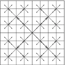
as r _{→ 0, to some set K ⊂ B(0, 1). Due to compactness results on the} Hausdorff convergence it is not difficult to have the existence of these limits up to subsequences. It is not even difficult to characterize their shapes: they can be only composed by up to three unit rays, which may form a diam-eter, a corner or triple 120◦ _{configuration when they are not a single ray}

(this up-to-subsequence result is proven in the chapter). What is not trivial at all is that these limits do not change according to the subsequence and this is proven with different techniques in different cases (endpoints, triple junctions. . . ): these techniques involve stationarity, small perturbations and Γ_{−convergence as well. Under an L}∞ assumption on the measure µ it is proven that at any point x0 ∈ Σ the full limit of the blow-up procedure

ex-ists. Moreover, in some cases it is possible to estimate the rate of change of the direction of the rays which form this limit, thus getting a C1,1 regularity result. This is proven in the last section of the chapter in a neighborhood of any point x0 such that the diameter of the set

T (x0) ={x ∈ Ω : d(x, Σ) = |x − x0|}

is sufficiently small. In particular this happens if x0 is a triple point, since

in this case we are able to prove that this set reduces to x0 only. In this

way we have a satisfactory description of the behavior of Σ near its triple junctions: it is composed by three C1,1 _{curves whose tangent vectors at}

x0 from three angles of 120◦. This gives a complete answer to one of the

(22)

regularity (partially answered by this blow-up result), asymptotics as l_{→ ∞} or l_{→ 0, boundary behavior and no-loop properties.}

Some of the techniques introduced in Chapter 8 are then used in Chapter 9 on a different problem. We come back to the branched transport frame-work and we want to study the blow-up. This has been first done by Xia in [74], and we know from it how the blow-up limits up to subsequences look like. In a work in progress with Jean-Michel Morel (see [61]) we try to use a curvature approach to deduce the existence of the limits: we fix a curve in the optimal network, we perturb it and we get optimality conditions. These conditions ensure that the derivative of the curve is a BV function on the interval of parametrization and allow to say that the curve has a side tangent vector at any point. This result requires some strong assumptions on the marginal measures, and in particular a lower bound on the densities. Here in this chapter we propose an alternative approach, which works under differ-ent conditions, which are less restrictive on the measures. We suppose that µ belongs to Lp(Ω) for a certain p > 1 and that the couple (µ, ν) satisfies the regularity assumption, i.e. either ν is atomic or spt(µ)_{∩ spt(ν) = ∅. On} the other hand, the result is only valid in two spatial dimensions and if the point x0 where to center the blow-up is a branching point (which is anyway

the most interesting case, since then we could apply some angle conditions). Under these conditions we are able to perform a procedure exactly as the one used in Chapter 8 for triple points. We prove that the oscillation of the angle θ(r) which represents the intersection direction of a branch of the optimal network N =_{{x ∈ Ω : [x]}η > 0} with ∂B(x0, r) may be estimated

by a quantity linked to the mass which is transported onto N ∩ B(x0, r).

Then it is sufficient to estimate this mass to get a convergence result and it is what we do, via some geometric and asymptotic estimates.

At the very beginning of the thesis there is a preliminary chapter on optimal transportation where all the results which will be useful later are introduced. There is no proof but only some bibliographical reference to the books by Villani, Ambrosio-Gigli-Savar´e and the lecture notes by Am-brosio ([71], [4] and [3], respectively). We deal with the primal and dual Kantorovich problems, with the existence of optimal maps, i.e. solutions to Monge’s problem, with the regularity of transports and potentials in the quadratic case by Monge-Amp`ere equation and with Wasserstein distances, curves in Wasserstein spaces, geodesics and geodesically convex functionals. As a whole, this thesis presents, in a quite unified setting of transport problems involving concentration criteria, almost all the researches that we carried out during these PhD studies. Only some subjects, mainly related to shape optimization, where the transport component was completely absent

(23)

has been neglected. Probably the most interesting feature of the thesis are the techniques to get necessary optimality conditions in the set of problems that have been approached. Most of them are not new; we simply use them in a particular way, obtaining sometimes unexpectedly strong results. This is the case of the derivation of some functionals on _{P(Ω) with respect of} perturbations such as µ + ε(µ1− µ) or (id + εξ)]µ. On the other hand some

regularization issues such as the L∞ one in Chapter 2 or the blow-up one in Chapter 8 have required some more technical tools which seem to be quite original. Moreover, also some very classical results, for instance from linear or nonlinear elliptic PDEs, from the theory of Campanato Spaces or from convex analysis, are used throughout the thesis and this completes the picture of the different techniques to get necessary conditions or regularity. Anyway, the thesis does not develop only this aspect of the variational prob-lems that approaches, but devotes also a certain space to the interpretation of the models (as in Chapters 1 and 2 for urban planning and in Chapter 7 for river basins) and to existence results (mainly in Chapter 4).

(24)

Notations

We summarize here most of the peculiar notations and expressions which are used throughout the thesis and not always explicitely recalled.

First, let us precise that we will call, for simplicity, domains those sets which are the closure of a non-empty connected and bounded open subset of Rd with negligible boundary. These domains will be often denoted by Ω, so that the reader must not be astonished if Ω denotes a compact set instead of an open one. Moreover, we will silently confuse a domain Ω and its interior Ω when some functional spaces involving higher regularity are◦ concerned: for instance when we write H1(Ω) we usually mean H1(Ω). This◦ is performed in order not to avoid heavy notations, should we distinguish between the closed and the open set.

Given a set C endowed with a natural topology (usually a domain) we will denote by_{P(C) the set of all Borel probability measures on C. The set} of finite vector on C measures valued inRk will be denoted by Mk_(C).

The d_{−dimensional Lebesgue measure will be denoted by L}d, but some-times we will write _{|Ω| for L}d_{(Ω). When we say “the Lebesgue measure}

on Ω”and we are speaking of a probability measure, we actually mean the rescaled measure 1/_{|Ω| · L}d restricted to Ω. The symbol _H1 will denote instead the 1_{−dimensional Hausdorff measure.}

For a sequence of probability or vector measures on Ω we will use the term weak convergence to mean the convergence in the duality with the space C0

b(Ω) of bounded continuous functions on Ω. This convergence will be

denoted by the symbol * (with no stars), so that µn* µ meansR_Ωφ dµn→

R

Ωφ dµ for any φ∈ Cb0(Ω).

Crucial will also be the concept of image measure: given a measure µ on Ω1 and a measurable map T : Ω1 → Ω2 we denote by T]µ the image of

µ through T , which is a measure on Ω2 defined by T]µ(A) = µ(T−1(A)) for

any measurable subset A_{⊂ Ω}2. If T]µ = ν we will also say that T transports

(25)

As far as more transport-related concepts are concerned, we denote by Π(µ, ν) the set of transport plans with marginal measures µ, ν_{∈ P(Ω) (see} Section 0.1) and by T P (µ, ν) the set of traffic plans from µ to ν. This latter concept is typical of the theory of branched transport: it consists of the set of all probability measures on the space of Lipschitz curves on [0, +_∞[ which eventually stop such that the images under the evaluation at the starting time and at the stopping time are µ and ν, respectively. These two evaluations are denoted by π0and π∞, respectively, as well as the evaluation

at a generic time t which is denoted by πt. See Section 6.2 for details.

The symbol id denotes the identity mapping from a set to itsels id(x) = x. The identity matrix is denoted by the symobl I. The symbol I the indicator function: if we write IA we mean the function whose value is 1 on

A and 0 outside. We may also write Icondition, which means a function of

possibly several variables whose value is 1 if the condition is verified and 0 otherwise. For instance, writing Ix∈γ is a function of two variables (x and

γ) which has the same values as Iγ(x). When a measure µ (usually the

Lebesgue or the Haudorff measures d _or_H1_{) and a set A are given, we will}

write IA· µ or µ A with the same meaning.

The indicator function in the sense of convex analysis is on the contrary denoted by a δ symbol: δ(_{·|A) is the function whose value is 0 on A and} +_{∞ elsewhere. Its Legendre-Flenchel transform is the support function of} A and it is given by δ∗(y|A) = supx∈Ay· x.

(26)

Preliminaries on Optimal

Transportation

This chapter does not want to be an exhaustive presentation of the topic, but only a short list of useful results with no proofs that will be used later on in thesis. The main reference is [71]. Anyway, the approach is the same used in the lectures given by Prof. L. Ambrosio at SNS Pisa in 2001/02 and hence another possible reference is [3].

The motivation for the whole subject is the following problem proposed by Monge in 1781 ([59]): given two densities of mass f, g _{≥ 0 on R}d_{, with}

R f = R g = 1, find a map T :_Rd_{→ R}d_{pushing the first one onto the other,}

i.e. such that Z

A

g(x)dx = Z

T−1_(A)

f (y)dy for any Borel subset A_{⊂ R}d and minimizing the quantity

Z

Rd|T (x) − x|f(x)dx

among all the maps satisfying this condition.

This problem has stayed with no solution (does a minimizer exist? how to characterize it?. . . ) for centuries. Only with the work by Kantorovich it has been inserted into a suitable framework which gave the possibility to approach it and, later, to find that actually solutions exist and to study them. The problem has been widely generalized, with very general cost functions c(x, y) instead of the euclidean distance|x − y| and more general measures and spaces. For simplicity, here we will not try to present a very wide theory on generic metric spaces, but we will deal only with the euclidean case.

(27)

0.1 Primal and dual problems

In what follows we will suppose Ω to be a domain of Rd and the cost func-tion c : Ω× Ω → [0, +∞[ will be supposed continuous and symmetric (i.e. c(x, y) = c(y, x)).

The generalization that appears as natural from the work of Kantorovich ([53]) of the problem raised by Monge is the following:

Definition 0.1.1. Given two probability measures µ and ν on Ω and a cost function c : Ω_{× Ω → [0, +∞] we consider the problem}

(K) min ½Z Ω×Ω c dπ_{|π ∈ Π(µ, ν)} ¾ , (0.1.1)

where Π(µ, ν) =_{{π ∈ P(Ω × Ω) : (p}+)]π = µ, (p−)]π = ν,} and p+ and p−

are the two projections of Ω_{× Ω onto Ω. The minimizers for this problem} are called optimal transport plans between µ and ν. Should π be of the form (id_{× T )}]µ for a measurable map t : Ω → Ω, the map T would be called

optimal transport map from µ to ν.

Remark 0.1.2. It can be easily checked that if (id_{× T )}]µ belongs to Π(µ, ν)

then T pushes µ onto ν (i.e. ν(A) = µ(T−1(A)) for any Borel set A) and the functional takes the form R c(x, T (x))µ(dx), thus generalizing Monge’s problem.

Remark 0.1.3. This generalized problem by Kantorovich is much easier to handle than the original one by Monge, for instance because in the Monge case we would need existence of at least a map T satisfying the constraints. This is not the case in the case µ = δ0 if ν is not a single Dirac mass.

On the contrary, there always exist transport plan in Π(µ, ν) (for instance µ_{⊗ ν ∈ Π(µ, ν)). Moreover, one can state that (K) is the relaxation of} the original problem by Monge: if one considers the problem in the same setting, where the competitors are transport plans, but sets the functional at +_{∞ on all the plans that are not of the form (id × T )}]µ, then one has a

functional on Π(µ, ν) whose relaxation is the functional in (K) (see [5]). An important tool will be duality theory and to introduce it we need in particular the notion of c−transform (a kind of generalization of the well-known Legendre transform).

Definition 0.1.4. Given a function χ : Ω _→ R we define its c−transform (or c_{−conjugate function) by}

χc(y) = inf

(28)

Moreover, we say that a function ψ is c_{−concave if there exists χ such that} ψ = χc _{and we denote by Ψ}

c(Ω) the set of c−concave functions.

It is well-known a duality result stating the following equality (see The-orem 1 together with the following Remark on c_{−concavity in [71]):}

Proposition 0.1.5. We have min(K) = sup ψ∈Ψc(Ω) Z Ω ψ dµ + Z Ω ψcdν. (0.1.2)

In particular the minimum value of (K) is a convex function of (µ, ν) as it is a supremum of linear functionals.

Definition 0.1.6. The functions ψ realizing the maximum in (0.1.2) are called Kantorovich potentials for the transport from µ to ν. This is in fact a small abuse, because usually this term is used only in the case c(x, y) =_|x−y| only.

Notice that any c−concave function shares the same modulus of continu-ity of the cost c. In particular, in the case c(x, y) =_{|x − y|}p, if Ω is bounded with diameter D, any ψ_{∈ Ψ}c(Ω) is pDp−1−Lipschitz continuous. The case

where c is a power of the distance is in fact of particular interest and two values of the exponent p are remarkable: the cases p = 1 and p = 2. In these two cases we provide characterizations for the set of c_−concave func-tions when Ω =Rd. Let us denote by Ψ(p)(Ω) the set of c−concave functions

with respect the cost c(x, y) =_{|x − y|}p/p. It is not difficult to check that ψ∈ Ψ(1)(Rd)⇔ ψ is a 1-Lipschitz function;

ψ∈ Ψ(2)(Rd)⇔ x 7→

x2

2 − ψ(x) is a convex function .

The first characterization is true also when Ω does not coincide with the whole space, while the second in fact becomes just an implication (if ψ ∈ Ψ(2), then x

2

2 − ψ(x) is convex, but not any convex function comes from a

c_{−concave function, due to the restriction on the Lipschitz constant).} The case c(x, y) =_{|x − y| shows a lot of interesting features, even if from} the point of the existence of an optimal map T it is one of the most difficult. A first interesting property is the following:

Proposition 0.1.7. For any 1_{−Lipschitz function ψ we have ψ}c=_{−ψ. In} particular, Formula 0.1.2 may be re-written as

min(K) = sup

ψ∈Lip₁

Z

Ω

(29)

Another peculiar feature of this case is the following:

Proposition 0.1.8. Consider the problem

(B) minnM (λ) : λ∈ Md(Ω);∇ · λ = µ − νo, (0.1.3) where M (λ) denotes the mass of the vector measure λ and the divergence condition is to be read in the weak sense, with Neumann boundary conditions, i.e. ₋_{R ∇φ · dλ = R φd(µ − ν) for any φ ∈ C}1_{(Ω). If Ω is convex then it}

holds

min(K) = min(B).

This proposition links the Monge-Kantorovich problem to a minimal flow problem which has been first proposed by Beckmann in [10], under the name of continuous transportation model, without knowing this link, as Kantorovich’s theory was being developed independently almost in the same years. In Section 2.1 we will see some details more on this model and on the possibility of generalizing it to the case of distances c(x, y) coming from Riemannian metrics. In particular, in the case of a nonconvex Ω, (B) would be equivalent to a Monge-Kantorovich problem where c is the geodesic distance on Ω.

We now come back to the case of a generic cost c(x, y). Another useful result about c−transform is the following:

Proposition 0.1.9. For any cost c and any function ψ : Ω → R we have ψcc_{≥ ψ and the equality holds if and only if ψ is c−concave.}

We summarize here some useful results for the case where the cost c is of the form c(x, y) = h(x_{− y), for a strictly convex function h.}

Theorem 0.1.10. Given µ and ν probability measures on a domain Ω⊂ Rd

there exists unique an optimal transport plan π. It is of the form (id_{× T )}]µ,

provided µ is absolutely continuous. Moreover there exists also at least a Kantorovich potential ψ, and the gradient∇ψ is uniquely determined µ−a.e. (in particular ψ is unique up to additive constants, provided the density of µ is positive a.e. on Ω). The optimal transport map T and the potential ψ are linked by T (x) = x− (∂h)−1₍_{∇ψ(x)). Moreover it holds ψ(x) + ψ}c_{(T (x)) =}

c(x, T (x)) for µ_{−a.e. x. Conversely, every map T which is of the form} T (x) = x_−(∂h)−1₍_{∇ψ(x)) for a function ψ ∈ Ψ}

c(Ω) is an optimal transport

(30)

Remark 0.1.11. Actually, the existence of an optimal transport map is true under weaker assumptions: we can replace the condition of being absolutely continuous by the condition µ(A) = 0 for any A⊂ Rd_{such that} _Hd−1_{(A) <}

+_{∞. Anyway, in this thesis only the absolutely continuous case will be used.} Remark 0.1.12. In Theorem 0.1.10 only the part concerning the optimal map t is not symmetric in µ and ν: hence the uniqueness of the Kantorovich potential is true even if it ν (and not µ) has positive density a.e.

Remark 0.1.13. Theorem 0.1.10 may be particularized to the quadratic case c(x, y) = _{|x − y|}2/2, thus getting the existence of an optimal transport map t = _{∇φ for a convex φ. By using the converse implication (sufficient} optimality conditions), this also proves the existence and uniqueness of a gradient of a convex function transporting µ onto ν. This well known fact has been investigated first by Brenier in [21].

All the costs c(x, y) =_{|x − y|}p _{with p > 1 fall under Theorem 0.1.10. For}

the case c(x, y) = |x − y| the results are a bit weaker and are summarized below (this is the classical Monge case and we refer to [5] and [45]).

Theorem 0.1.14. Given µ and ν probability measures on a domain Ω⊂ Rd

there exists at least an optimal transport plan π. Moreover, one of such plans is of the form (id_{× T )}]µ provided µ is absolutely continuous. There exists

also at least a Kantorovich potential ψ, and we have ψ(x)− ψ(T (x)) = |x − T (x)| for µ−a.e. x, for any choice of optimal T and ψ.

Here the absolute continuity assumption is essential to have existence of an optimal transport map, in the sense that in general it cannot be replaced by weaker assumptions as in the strictly convex case. This can be seen from the following example.

Example 0.1.15. Set

µ =H1 A and ν = H

1 _{B +}_H1 _C

2

where A, B and C are three vertical parallel segments in_R2 _{whose vertexes}

lie on the two line y = 0 and y = 1 and the abscissas are 0, −1 and 1, respectively. In this case one can get a sequence of maps Tn: A→ B ∪ C by

dividing A into 2n equal segments (Ai)i=1,...,2nand B and C into n segments

each, (Bi)i=1,...,n and (Ci)i=1,...,n (all ordered upwards). Then define Tn as

a piecewise affine map which sends A2i−1 onto Bi and A21 onto Ci. In this

way the cost of the map Tn is less than 1/2 + 1/n, but no map T may

(31)

and but this cannot respect the push-forward constraint. On the other hand, the transport plan associated to Tn weakly converge to the transport plan

1/2T_]+µ + 1/2T_]−µ, where T±(x) = x± e and e = (1, 0). This transport plan turns out to be the only optimal transport plan and has a Kantorovich cost of 1/2.

The same construction provides also an example of the relaxation pro-cedure leading from Monge to Kantorovich.

0.2 Wasserstein distances and spaces

Starting from the values of the problem (K) in (0.1.1) we can define a set of distances over_{P(Ω). For any p ≥ 1 we can define}

Wp(µ, ν) =¡ min(K) with c(x, y) = |x − y|p

¢1/p . We recall that it holds, by Duality Formula,

1 pW p p(µ, ν) = sup ψ∈Ψp(Ω) Z Ω ψ dν + Z Ω ψcdµ. (0.2.1)

Theorem 0.2.1. If Ω is compact, for any p ≥ 1 the function Wp is in

fact a distance over_{P(Ω) and the convergence with respect to this distance} is equivalent to the weak convergence of probability measures. In particular any functional µ7→ Wp(µ, ν) is continuous with respect to weak topology.

The case of a noncompact Ω is a little more difficult. First, the distance must be defined only on a subset of the whole space of probability measures, to avoid infinite values. We will use the space of probabilities with finite p−th momentum:

Wp(Ω) ={µ ∈ P(Ω) : Mp(µ) :=

Z

Ω|x|

p_{µ(dx) < +}_∞}.

Theorem 0.2.2. For any p≥ 1 the function Wp is a distance over Wp(Ω)

and, given a measure µ and a sequence (µn)n in Wp(Ω), the following are

equivalent: • µn→ µ according to Wp; • µn* µ and Mp(µn)→ Mp(µ); • R Ωφ dµn → R

Ωφ dµ for any φ ∈ C0(Ω) whose growth is at most of

order p (i.e. there exist constants A and B depending on φ such that φ(x)≤ A + B|x|p _{for any x).}

(32)

Notice that, as a consequence of H¨older inequalities, the Wasserstein distances are always ordered, i.e. Wp1 ≤ Wp2 if p1 ≤ p2. Reversed

in-equalities are possible only if Ω is bounded, and in this case we have, if set D = diam(Ω), for p1≤ p2,

Wp1 ≤ Wp2 ≤ D

1−p1/p2_Wp1/p2

p1 .

From the monotone behavior of Wasserstein distances with respect to p it is natural to introduce the following distance W∞: set W∞(Ω) =

{µ ∈ P(Ω) : spt(µ) is bounded } (obviously if Ω itself is bounded one has_W∞(Ω) =P(Ω)) and then

W∞(µ, ν) = inf ( π_{− ess sup} x,y∈Ω×Ω|x − y| : π ∈ Π(µ, ν) ) .

It is easy to check that Wp% W∞ and it is interesting to study the metric

space _W∞(Ω). Curiously enough, this supremal problem in optimal

trans-port theory, even if quite natural, has not deserved much attention up to now.

The W∞ convergence is stronger than any Wp convergence and hence

also than the weak convergence of probability measures. The converse is not true and W∞ converging turns out to be actually rare: consequently

there is a great lack of compactness in _W∞. For instance it is not difficult

to check that, if we set µt= tδx0 + (1− t)δx1, where x0 6= x1 ∈ Ω, we have

W∞(µt, µs) =|x0−x1| if t 6= s. This implies that the balls B(µt,|x0−x1|/2)

are infinitely many disjoint balls in_W∞ and prevents compactness.

The following statement summarizes the compactness properties of the spaces Wp for 1≤ p ≤ ∞ and its proof is a direct application of the

consid-erations above and of Theorem 0.2.2.

Proposition 0.2.3. For 1≤ p < ∞ the space Wp(Ω) is compact if and only

if Ω itself is compact. Moreover, for an unbounded Ω the space Wp(Ω) is

not even locally compact. The space W∞(Ω) is neither compact nor locally

compact for any choice of Ω with ]Ω > 1.

0.3 Geodesics, continuity equation and

displace-ment convexity

We are concerned in this sections with several properties linked to the curves in the Wasserstein space Wp. For this subject the main reference is [4].

(33)

Before giving the main result we are interested in, we recall the definition of metric derivative, which is a concept that may be useful when studying curves which are valued in generic metric spaces.

Definition 0.3.1. Given a metric space (X, d) and a curve γ : [0, 1] _{→ X} we define metric derivative of the curve γ at time t the quantity

|γ0|(t) = lim

s→t

d(γ(s), γ(t))

|s − t| , (0.3.1) provided the limit exists.

As a consequence of Rademacher Theorem it can be seen (see [7]) that for any Lipschitz curve the metric derivative exists at almost every point t_{∈ [0, 1]. We will be concerned quite often with metric derivatives of curves} which are valued in the spaceWp(Ω).

Definition 0.3.2. If we are given a Lipschitz curve µ : [0, 1]_{→ W}p(Ω), we

define velocity field of the curve any vector field v : [0, 1]× Ω → Rd _such

that for a.e. t _{∈ [0, 1] the vector field v}t = v(t,·) belongs to [Lp(µt)]d and

the continuity equation

d

dtµt+∇ · (v · µt) = 0

is satisfied in the sense of distributions: this means that for all φ∈ C1 c(Ω)

and any t1 < t2 ∈ [0, 1] it holds

Z Ω φ dµt2 − Z Ω φ dµt1 = Z t₂ t1 ds Z Ω∇φ · vs dµs,

or, equivalently, in differential form: ∂ ∂t Z Ω φ dµt= Z Ω∇φ · vt dµt for a.e. t∈ [0, 1].

We say that v is the tangent field to the curve µtif, for a.e. t, vthas minimal

[Lp(µt)]d norm for any t among all the velocity fields.

The following proposition is concerned with the existence of tangent fields and comes from Theorem 8.3.1 and Proposition 8.4.5 in [4].

(34)

Theorem 0.3.3. If p > 1 and µ = (µt)t is a curve in Lip([0, 1]; Wp(Ω))

then there exist unique a tangent vector field v, and it is characterized by ∂

∂tµ +∇ · (v · µ) = 0, (0.3.2) ||vt||Lp_(µ

t)≤ |µ

0_{|(t) for a.e. t,} _(0.3.3)

where the continuity equation is satisfied in the sense of distributions as previously explained. Moreover, if (0.3.2) holds for a family of vector fields (vt)twith||vt||Lp_(µ

t) ≤ C then µ ∈ Lip([0, 1]; Wp(Ω)) and|µ

0_{|(t) ≤ ||v} t||Lp_(µ

t)

for a.e. t.

This characterization of Lipschitz (or, up to reparameterization, abso-lutely continuous) curves in Wp will be very useful in Chapter 5. Moreover,

in the general theory of Wasserstein spaces, it is a key instrument for study-ing geodesics and other properties linked to them, which will be used in Chapters 2, 5, 6 and 7.

The following result is a characterization of geodesics in Wp(Ω) when Ω

is a convex domain in Rd (see Proposition 7.2.2 in [4], but some extension to the case of length spaces, for instance non convex domains, may be found in [54]). This procedure is also known as McCann’s linear interpolation. Theorem 0.3.4. All the spaces _Wp(Ω) are length spaces and if µ and ν

belong to Wp(Ω), any geodesic curve linking them, when parametrized by

arc-length, is of the form

γπ(s) = (ps)]π

where ps : Ω× Ω → Ω is given by ps(x, y) = x + s(y− x) and π is an optimal

transport plan from µ to ν for the cost cp(x, y) =|x − y|p. In the case p > 1

and µ, ν absolutely continuous, if T is the corresponding optimal transport map such that π = (id× T )]µ,then the curve has the form

γπ(s) = [(1_{− s)Id + sT ]}#µ.

Conversely, any curve of this form, for a transport plan π or a transport map T , is an arc-length geodesic.

By means of this characterization of geodesics we can also define the useful concept of displacement convexity introduced by McCann in [58]. Definition 0.3.5. Given a functional F : Wp(Ω)∩ L1 → [0, +∞], we say

that it is displacement convex if all the maps t _{7→ F (γ}π(t)) are convex on [0, 1] for every choice of µ and ν in _Wp(Ω) and π optimal transport plan