Comparison of Machine Learning Methods Applied to SAR Images for Forest Classification in Mediterranean Areas

(1)

Article

Comparison of Machine Learning Methods Applied to

SAR

Images

for

Forest

Classification

in

Mediterranean Areas

Alessandro Lapini 1,_{*, Simone Pettinato}1_{, Emanuele Santi} 1_{, Simonetta Paloscia}1_,

Giacomo Fontanelli 1_{and Andrea Garzelli}2 1_{Institute of Applied Physics – National Research Council of Italy (IFAC – CNR), Via Madonna del Piano} 10, 50019 Florence, Italy 2_{Department of Information Engineering and Mathematics, University of Siena, 53100 Siena, Italy} * Correspondence: a.lapini@ifac.cnr.it; Tel.: +39 055 5226460 Received: 18 November 2019; Accepted: 17 January 2020; Published: 22 January 2020

Abstract: In this paper, multifrequency synthetic aperture radar (SAR) images from ALOS/PALSAR, ENVISAT/ASAR and Cosmo‐SkyMed sensors were studied for forest classification in a test area in Central Italy (San Rossore), where detailed in‐situ measurements were available. A preliminary discrimination of the main land cover classes and forest types was carried out by exploiting the synergy among L‐, C‐ and X‐bands and different polarizations. SAR data were preliminarily inspected to assess the capabilities of discriminating forest from non‐forest and separating broadleaf from coniferous forests. The temporal average backscattering coefficient (𝜎°) was computed for each sensor‐polarization pair and labeled on a pixel basis according to the reference map. Several classification methods based on the machine learning framework were applied and validated considering different features, in order to highlight the contribution of bands and polarizations, as well as to assess the classifiers’ performance. The experimental results indicate that the different surface types are best identified by using all bands, followed by joint L‐ and X‐ bands. In the former case, the best overall average accuracy (83.1%) is achieved by random forest classification. Finally, the classification maps on class edges are discussed to highlight the misclassification errors.

Keywords: SAR; Mediterranean forests; forest features; forest/non‐forest areas; land classification; machine learning

1. Introduction

Forest monitoring is commonly recognized as a vital task due to the role played by these ecosystems in carbon cycle evolution, which act as the main terrestrial carbon sinks [1]. Since maps of forest status and their temporal evolution are increasingly required, the combined use of in‐situ and remote sensing data is desirable, especially in regions with scarce accessibility and limited ground data availability [2]. Optical sensors have been widely used for a long time, although these sensors have the limitation of operating in clear‐sky conditions and are sensitive to the upper layer of the canopy only (e.g., [3,4]). This makes the investigation of equatorial, boreal and mountain areas rather difficult, due to the frequent and consistent cloud cover. Microwave frequencies have the advantage to be independent of cloud cover and solar radiation and can significantly penetrate vegetation canopy. Both emission and backscatter are considerably influenced by moisture content and by the geometrical features of plant constituents, according to frequency and polarization. A very suitable sensor for forest investigations is the synthetic aperture

(2)

radar (SAR), which was carried onboard historical satellites, such as ALOS‐1, RADARSAT‐1 and ENVISAT, and subsequently launched ones, e.g., Cosmo‐SkyMed, TerraSAR‐X, ALOS‐2, RADARSAT‐2 and Sentinel‐1. The total backscatter from a forest is a combination of contributions from ground, vegetation components and their interactions. Each of these components affects the total scattering depending on the microwave wavelength, polarization and incidence angle. At wavelengths shorter than 10 cm, i.e., 5.6 cm (C‐band) and 3 cm (X‐band), the backscatter is mainly due to leaves or needles and twigs of the upper canopy. This makes it possible to obtain information on the upper layer of vegetation cover, allowing the identification of forest/non‐forest areas [5–12]. Longer wavelengths, i.e., 21 cm (L‐band) and 60 cm (P‐band), provide us information on thicker layers of vegetation and of soil under vegetation cover, due to the higher penetration power of radar intensity and to the interactions with major branches, trunks and ground [13–16]. Experimental and theoretical investigations carried out for many years mainly focused on the use of SAR systems for the monitoring of boreal forests of North America and Eurasia (in view of their influence on climate changes [17,18]) and of tropical regions, due to the frequent cloud cover that hampers the use of optical sensor [14,19,20]. Interesting recent works have been carried out by Deutcher et al. [21] and Perko et al. [22] on tropical rainforests and European forest sites by using high‐resolution (Spotlight) X‐band data, in order to estimate the tree height by using interferometric methods. The estimation of forest features in Mediterranean areas by means of SAR images is a complex task: the vegetation cover is spatially fragmented and heterogeneous due to the long‐term effect of human activities. The variable aridity conditions, typical of the Mediterranean climate, represent an additional challenge, since they irregularly limit foliage density, creating incomplete and discontinuous plant canopies that are difficult to characterize from remote sensing observations [23]. Similar investigations were performed in [24] by using support vector machine classification on the test site of the entire Tasmania. The kind of forest and the age of the plantations were quite diversified in comparison with the San Rossore test site, while the classifier algorithm was implemented to discriminate only two output classes, i.e., forest and non‐forest. The best results were obtained with L‐band, obtaining and overall accuracy of 92.1%. However, it must be remarked that the nature of the forest in Tasmania is substantially different than the one present in the Mediterranean areas.

The aim of this research is to investigate the sensitivity of multi‐frequency, multi‐polarization SAR data to Mediterranean forest characteristics and to identify the role of each frequency in the assessment of forest classification. A few research works have been focused on the investigation of Mediterranean forests, but specifically aiming at studying forest fire events and the successive re‐ growth of biomass (e.g., [25,26]). This study, which can be considered as a preparatory step in evaluating the image information content in view of the estimate of growing stock volume, deals with the exploitation of SAR backscatter capabilities for classifying forest types in Mediterranean areas. A forest area, which is a coastal plain mostly covered by evergreen conifers located in Central Italy (San Rossore), is examined. In this area, a forest classification map was available together with ground measurements of forest parameters. SAR images were acquired from ALOS/PALSAR (L‐band), ENVISAT/ASAR (C‐band) and Cosmo‐SkyMed (X‐ band) systems. SAR data are used to discriminate forest from non‐forest land covers and separating broadleaved from coniferous forest types by using compositions of multi‐temporal and multi‐frequency images. A preliminary analysis of SAR image compositions by using various frequencies and polarizations is carried out to highlight the discriminating capability of ALOS/PALSAR, ENVISAT/ASAR and Cosmo‐SkyMed data. Pixels associated to different cover areas are detected by means of the in‐situ map and the corresponding temporal average backscattering coefficients (𝜎°) are evaluated. The classification of different areas is then performed by supervised machine learning techniques applied to the radiometric values. The originality of the research relies on the application of multi‐frequency SAR images to heterogeneous and mixed forests of Central Italy and on the related performance comparison of different classifiers. Due to specific peculiarity of the targets, the classification process must overcome the limits of ground‐truth classes that contain not homogenous targets (i.e., non‐forest class). This peculiarity can

(3)

be considered innovative with respect to conventional classification of multi‐polarization/multi‐ frequency SAR images. Moreover, the role of each frequency is better identified by integrating the different contributions.

The paper is organized as follows: 1) description of the test area and the experimental data; 2) description of the methods applied to the SAR images for the analysis and the classification of Mediterranean forests; 3) results; 4) discussion and 5) conclusions.

2. Test Area and Input Data

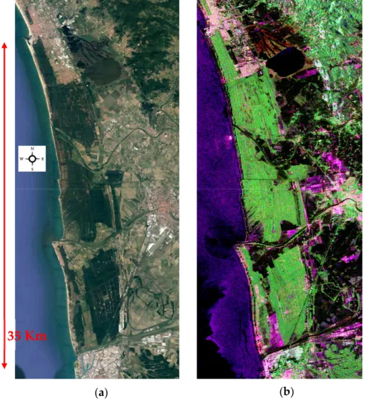
The investigation was carried out in a forest area in Central Italy, where ground measurements, meteorological information and other ancillary data were available (see Figure 1). The natural park of San Rossore (43.72°N, 10.30°E) is a protected flat area of about 4800 ha located along the coast of Tuscany Region. The area is covered by forests and pastures; forests are dominated mainly by Mediterranean pines (Pinus pinaster Ait. and Pinus pinea L.) and deciduous broadleaf (i.e., Quercus

robur L., Fraxinus subsp. oxycarpa M. Bieb. ex Wild, Ulmus laevis Miller, Alnus glutinosa (L.) Gaertner,

etc.). The ground truth is represented by the forest type map produced by ‘Dimensione Ricerca Ecologia Ambiente’, DREAM (2003) [27] and it is reported in Figure 2. The original classification map was provided at the 1:15000 scale and was derived from field observations collected in the whole Park. According to the definition used by the Tuscany Regional authority, forests correspond to areas having a minimum extension of 2000 m2_{, a length greater than 20 m, and tree cover must be greater} than 20%. Unfortunately, evergreen broadleaf forests (dominated by Holm oak, Quercus ilex L.) cover only a marginal area (0.2%) of the whole Park, thus, it was not possible to separate them to coniferous and deciduous broadleaf forests. Logging activities had an interested part of the forest area since 2009; therefore, a preliminary check was done to exclude these areas from the training and the test phases. Felled areas were identified using a Landsat TM of 2009 and Google Earth images of 2010. Additional conventional measurements were carried out on 72 forest stands covered by three forest species groups: Mediterranean pines, holm oak and deciduous trees, whose area ranged from 1 to 170 ha [28]. Figure 1. Italian forest test area of San Rossore in Tuscany (from Google Earth).

35 Km

(4)

Figure 2. Forest type map produced by DREAM [27]. Red: coniferous, Green: broadleaf, Blue: Non‐

forest, Black: unclassified.

A series of SAR images, listed in Table 1, was collected at L‐(ALOS/PALSAR), C‐ (ENVISAT/ASAR) and X‐(COSMO‐SkyMed) bands in 2009 and 2010 across different seasons and by using different modality of observation. The original (range, azimuth) resolution of the PALSAR, ASAR and COSMO‐SkyMed images were (9.3 m, 6.1 m), (7.8 m, 4.0 m) and (1.1 m, 1.9 m), in that order. Furthermore, the images are characterized by different incidence angle, polarization, acquisition mode and daily time acquisition, as reported in Table 1.

(5)

Table 1. Synthetic aperture radar (SAR) images available in the test area of San Rossore. Data are

grouped according to time closeness.

Group Sensor Date Time (UTC) Pass. Inc. Ang. Pol. Mode

1

PALSAR 28/02/2009 21:43:00 Asc 38 HH FBS ASAR 26/02/2009 09:38:29 Desc 23 VV IMS

CSK2 06/03/2009 05:13:15 Asc 33 HH Himage 2

PALSAR 07/06/2009 21:03:08 Asc 22 HH/HV/VH/VV POL ASAR 26/05/2009 20:59:38 Asc 23 VV IMS CSK2 25/05/2009 05:12:24 Asc 33 HH Himage 3

PALSAR 29/06/2009 21:41:48 Asc 38 HH/HV FBD ASAR 27/06/2009 09:35:57 Desc 23 VV IMS CSK2 25/05/2009 05:12:24 Asc 33 HH Himage 4

PALSAR 16/10/2009 21:44:25 Asc 38 HH/HV FBD ASAR 13/10/2009 20:59:34 Asc 23 VV IMS

CSK *N/A * * *

7

PALSAR 30/12/2009 21:42:15 Asc 38 HH FBS ASAR 22/12/2009 20:59:34 Asc 23 VV IMS

CSK *N/A * * * *

8

PALSAR 16/01/2010 21:44:22 Asc 38 HH FBS ASAR 10/01/2010 21:02:24 Asc 23 VV IMS

CSK2 20/01/2010 05:09:38 Asc 33 HH Himage 9

CSK2 21/02/2010 05:09:15 Asc 33 HH Himage 10

CSK2 25/03/2010 05:08:25 Asc 33 HH Himage 11

CSK *N/A * * * *

12

PALSAR 19/07/2010 21:42:52 Asc 38 HH/HV FBD ASAR 20/07/2010 20:59:36 Asc 23 VV IMS

CSK *N/A * * * *

3. Methods

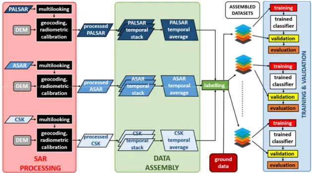
This investigation aims at evaluating the use of the available SAR data for discriminating forest from non‐forest land covers and separating broadleaved from coniferous forest types. The processing flow, presented in this section, is visually synthesized in Figure 3.

(6)

Figure 3. Processing flow of the proposed approach.

3.1. Data Preprocessing and Analysis

A preliminary analysis, aiming at understanding the role of each frequency in the assessment of forest features, was carried out. All the available SAR images were pre‐processed by using SARSCAPE©. The original image dataset was collected in single‐look complex slant range format, which does not include radiometric corrections. The pre‐processing description of the procedure follows.

First, the radiometric calibration was performed using a digital elevation model (DEM) [29]. The radiometric correction provided imagery in which pixel values truly represent the radar backscatter of the reflecting surface. This step is necessary for the comparison of SAR images acquired with different sensors or from the same sensor but at different times and modes or for scenes processed by different processors. Subsequently, multilooking was applied to reduce the speckle impairments. Since SAR sensors have different spatial resolutions, the window size must vary accordingly. Specifically, window sizes (in range and azimuth, respectively) of 1 pixels × 2 pixels (PALSAR), 1 pixels × 5 pixels (ASAR) and 2 pixels × 2 pixels (CSK2) were adopted. Successively, since the SAR images were in the 2D raster radar geometry (i.e., slant range view), a precise geolocation process was applied by using orbit state vector information, radar timing annotations, the slant to ground range conversion parameters and the reference DEM data. The resulting geocoded images had a pixel size of 10 m × 10 m and the same projection (UTM 32N). Finally, the SAR images were co‐registered by shifting each image in the stack file by using ENVI©, in order to relate the same pixel to the same geocoded target and allowing a ‘pixel by pixel’ comparison among the various images and the ground truth.

Afterwards, some RGB compositions, derived from the available SAR images of Table 1, were prepared for each area in order to visually inspect the classification capability of different frequencies. RGB images were compared with the available ground truth. As an example, in Figure 4b, an RGB visualization of ALOS/PALSAR images collected on San Rossore area in 7th June 2009 at three polarizations is shown (R: HH pol., G: HV pol. and B: VV pol.), which allows a preliminary but clear identification of forest areas with respect to other type of surfaces. In Figure 4a, an optical Google Earth image is also shown for a visual match. Comparing both images, forest areas recognizable in the Google Earth image correspond to green pixels in the RGB composite, pointing out the importance of HV polarization in identification of forest areas. Indeed, cross polarization at the L‐ band was mainly sensitive to inclined cylinders of dimensions comparable to the carrier radar

(7)

wavelength (about 20 cm) and therefore represented by thick branches and trunks. When inclined cylinders were observed, the backscattering coefficient shows a maximum whose position tended toward lower diameter values as the frequency increased [10,30]. For each frequency the range of diameters producing the maximum values of the backscatter coefficient was a fraction of the wavelength (1/10‐1/20).

Figure 4. RGB image of San Rossore area on top right side, (a) compared with a Google Earth image

and (b) PALSAR quadpol 7/6/2009. Color legend for (b): R: HH, G: HV and B: VV.

3.2. Temporal Average Backscatter Images

The image dataset for classification was built starting from all the available data reported in Table 1, with the only exception of quad‐pol PALSAR acquisition that had been excluded a‐priori for sake of consistency with the other SAR data in terms of incidence angle and type of product. The co‐ registered image stack had been initially split in four sub‐stacks, namely PALSAR HH, PALSAR HV, ASAR VV and CSK2 HH, grouping together the images sensed by the same sensor and the same polarization. The statistics of the backscattering coefficient evaluated over each sub‐stack for coniferous and broadleaf forests are reported in Table 2. The mean backscattering values were close (gap of about 0.5 dB) in PALSAR HH and PALSAR HV, whereas they increase for broadleaf with respect to coniferous (gap greater than 1.5 dB) in ASAR VV and CSK2 HH. Hence, the different sensitivities at various frequencies to forest characteristics were well pointed out. At X‐ and C‐bands, the operative wavelength (between 3 and 6 centimeters, respectively) was comparable with the

(b)

(a)

(8)

dimensions of needles and leaves, being more sensitive these surface characteristics. On the other hand, at L‐band, the longer wavelength (about 20 cm) had a higher penetration power inside vegetation cover and was less influenced by crown characteristics. Furthermore, by considering the standard deviation of each sub‐stack, it emerged that the horizontal polarization (PALSAR HH and CSK2 HH) exhibited the highest dispersion. Interestingly, if the median absolute deviation (M.A.D.) was used instead of the standard deviation, the contribution of speckle and outliers was reduced (up to –3.99 dB for the broadleaf class in PALSAR HH). Thus, a limited temporal dispersion of data for sensor‐polarization pair was assumed.

The images of each sub‐stack were subsequently averaged, in order to obtain four temporal average backscatter coefficient images. This processing was motivated by two reasons: i) improve the signal intensity with respect to speckle noise and ii) minimize the seasonal effects (such as soil moisture variations, presence/absence of leaves, higher or lower tree water content) on the classification procedures. As to the effects of soil moisture, model simulations in [31] pointed out that for high cover fraction, typical of the most of the plots of the San Rossore forest, the soil contribution becomes negligible at L‐band for growing stock volume values higher than 50 m3_/ha.

Table 2. Statistics of the backscattering coefficient computed for each image sub‐stack, discriminating

between coniferous and broadleaf according to Figure 2.

Sub‐stack Coniferous Broadleaf Coniferous Broadleaf Coniferous Broadleaf Mean 𝜎° (dB) St. Dev. 𝜎° (dB) M.A.D. 𝜎° (dB) PALSAR HH −8.51 −8.11 −10.67 −9.60 −13.53 −14.59 PALSAR HV −14.03 −14.59 −16.83 −17.51 −19.03 −19.87 ASAR VV −9.70 −8.12 −11.81 −14.56 −14.68 −16.50 CSK2 HH −9.37 −7.20 −12.63 −11.10 −15.43 −13.13 Radiometric discrimination among classes was preserved in the temporal average backscattering coefficient images. This fact can be appreciated, for instance, by visual inspecting the PALSAR HH and PALSAR HV images, reported in Figure 5a,b, respectively. Different forest features could be weakly identified in the former image; instead, they were visible in the latter, due to the presence of inclined cylinders represented by branches and trunks. However, also in this case, the discrimination between the two types of forest was not trivial. In Figure 5c,d, ASAR VV and CSK2 HH images were respectively represented; in these images, the features inside the forest area were more evident than in the previous ones, and the temporal average backscatter coefficient seemed more suitable to discriminate coniferous and broadleaf forests.

(9)

Figure 5. Temporal average backscattering coefficient 𝜎° images computed over the San Rossore test site for each SAR sensor and polarization available from the dataset of Table 1. The red line identifies the contour of forest area, derived from the map produced by DREAM of Figure 3. (a) PALSAR HH; (b) PALSAR HV; (c) ASAR VV and (d) CSK2 HH. The additional contribution of interferometric coherence [32] for classification purposes was also investigated. Nevertheless, it was not reported in this work because no relevant improvement emerged in our test cases.

3.3. Classification Dataset

The classification dataset was obtained by stacking the temporal average backscattering coefficient images described in Section 3.2. For convenience, the composition of the classification stack is listed in the following: 1. PALSAR HH stack, which is the temporal average of 11 HH polarized PALSAR images collected from single and dual polarization acquisitions; 2. PALSAR HV stack, which is the temporal average of 5 HV polarized PALSAR images collected from dual polarization acquisitions; 3. ASAR VV stack, which is the temporal average of 12 HV polarized ASAR images; 4. CSK2 HH stack, which is the temporal average of 7 HH polarized CSK2 images.

(a)

(b)

(c)

(d)

(10)

The classification of SAR images is generally impaired by speckle noise. Even though the multitemporal averaging intrinsically introduces a speckle reduction, a performance margin was empirically observed when applying a despeckling stage, especially for the smallest temporal stack (PALSAR HV). Thus, a 7 × 7 sliding window Kuan filter was applied to each image of the classification stack, as a tradeoff between speckle removal and reduced computational burden [33]. After masking of unclassified and no‐data‐pixel, a total of 365,541 labeled samples were extracted. The prior distribution of the labeled samples is the following: coniferous (39.4%), broadleaf (41.3%) and non‐forest (19.3%). Each sample is a four‐element vector whose components were the temporal average backscattering coefficients evaluated at the same pixel in the classification stack. The sample label was the class (coniferous, broadleaf and non‐forest) of the corresponding pixel according to the reference map (Figure 2). In Figure 6, the distributions related to PALSAR HV and the CSK2 HH components collected in the classification dataset are shown. It can be observed that coniferous and broadleaf classes were distributed according to monomodal distributions with a high degree of symmetry. On the contrary, the non‐forest class was remarkably asymmetric. This is explained by considering the heterogeneity of this class, where different surface features as marine environment, agricultural fields and small anthropic settlements are contained. By visual inspection, it can be noted that coniferous and broadleaf classes were better distinguished in the X‐band (Figure 6b), whereas non‐forest was more separated in the C‐band (Figure 6a). The improvement in terms of separation among classes when using of three components, namely PALSAR HV, CSK2 HH and PALSAR HV, could be appreciated in Figure 6c, where the joint three‐dimensional distribution was reported. Thus, an improvement in the performance of classifiers is expected by using the bands jointly.

(11)

(a) (b)

(c)

Figure 6. Distributions of the pixel values collected in the classification dataset separated by class

(coniferous, broadleaf and non‐forest), (a) histogram of PALSAR HV data; (b) histogram of CSK2 HH data and (c) 3‐D scatterplot of PALSAR HV‐CSK2 HH‐PALSAR HV data. 3.4. Image Classification Methods The classification of the test site was carried out by using the following supervised classification methods belonging to the machine learning framework:  Random forest (RF);  AdaBoost with decision trees (AB);  K‐nearest neighbors (kNN);  Feed forward artificial neural networks (FF‐ANNs);  Support vector machines (SVM);  Quadratic discriminant (QD). Random forest (RF) is a classification method belonging to the ensemble learning methods [34]. Ensemble classifiers perform decisions by aggregating the classification results coming from several weak classifiers. In RF, the weak classifiers are decision trees [35] and predictions are performed by the majority, i.e., the predicted class is the most voted by all the weak classifiers. Decision trees are trained by randomly drawing with replacement a subset of training data (bagging). The RF algorithm

(12)

has been demonstrated to reduce both the bias and the overfitting with respect to decision trees, as well as making unnecessary the pruning phase [36]. Two main parameters must be set in RF: the number of features in the random subset at each node and the number of decision trees [37]. All these aspects, as well as a contained computation burden (compared, for instance, to SVM) and outperforming classification results, have contributed to make RF very popular in the study of land cover, too (see, for instance, [36–40]).

Boosting algorithms generally refer to the method that combines weak classifiers to get a strong classifier [41]. AdaBoost with decision trees (AB) [42] is a boosting ensemble classification method whose prediction relies on a weighted mean of the outputs of several weaker decision trees (the higher the weight, the more reliable the decision tree). The iterative training algorithm selects a decision tree at each step, in order to minimize a cost function, and update the weights. This process has been shown to improve the overall performance under some optimality measure [42]. AdaBoost has been already considered in the remote sensing literature, e.g., for tree detection [43], land cover classification in tropical regions [44] and land cover classification carried out on hyperspectral images [45]. Nevertheless, the main drawbacks of AB are its sensitivity to outliers and the number of hyperparameters to be optimized in order to improve the classification performance.

The K‐nearest neighbors (KNN) algorithm is another popular classification method [46]. In KNN, the training dataset corresponds to a set of labeled points in the space of features. The prediction is performed by only considering the classes of the k training samples that are closest to test sample, according to a given metric. There are many strategies to perform this decision, e.g., majority vote, weighted distance [47] or by using Dempster–Schafer theory [48]. An integration of KNN and SVM has been also proposed [49]. The basic KNN algorithm usually attains suboptimal classification performance compared to other more recent methods and can be memory intensive for a high number of features. Nevertheless, due its plain logic and configuration (the main parameter is the number of neighbor k), it has been thoroughly used as benchmark in the remote sensing community [39,50,51].

An algorithm based on feed forward artificial neural networks (FF‐ANNs) has been also considered for the comparison. FF‐ANN is conceived for establishing non‐linear relationships between inputs and outputs [52] and therefore cannot be regarded as a classification algorithm strictly speaking. However, they can be applied to almost any kind of input–output relationships and their ability in solving non‐linear problems has been largely proven [53]. FF‐ANN is composed of a given number of interconnected neurons, distributed in one or more hidden layers, that receive data, perform simple operations (usually additions and products) and propagate the results. The FF‐ANN training is based on the back propagation (BP) learning rule, which is a gradient descendent algorithm aimed at minimizing iteratively the mean square error (MSE) between the network output and the target value. As a main disadvantage, FF‐ANN is sensitive to outliers: a training representative of the testing conditions is therefore mandatory for obtaining satisfactory results [54]. In this study, FF‐ANN was adapted to act as classifiers by simply rounding the obtained outputs to the closest integer.

Another popular algorithm for classification is represented by support vector machine (SVM). In SVM, the space of features is divided in subspaces by means of hyperplanes, named decision planes, and the prediction is performed according to the subspace that the test point belongs to (see, for instance, [55]). The decision planes are computed during the training phase searching for the maximum margin, according to some distance function. SVM have been also extended to deal with nonlinear separation hypersurfaces [55,56], allowing us to map the features in a higher‐dimensional feature space through some nonlinear mapping and formulating a linear classification problem in that feature space by means of kernel functions. SVM‐based methods are very common due to their good classification performance (see, for instance, [24,37,39,40,50,57]). As a drawback, SVM may require a fine tuning of many hyperparameters to obtain the optimal result. Furthermore, the training of SVM classifiers is performed by means of quadratic programming optimization routines [55]; thus, the training time is usually higher than, for instance, RF.

(13)

The quadratic discriminant classifier (QD) pertains to the discriminant analysis framework [58]. In QD, data samples are assumed to be generated according to a Gaussian mixture distribution. The mean and the covariance matrix of each component are estimated by using the training data set belonging to the corresponding class. The prediction is performed by computing the posterior probability that the test sample belongs to each class and selecting the class for which the maximum is attained. Despite of the simplistic statistical hypothesis, QD can often deal with complex data models, exhibiting a competitive classification performance [59,60]. Furthermore, the training and decision phases are usually extremely fast.

4. Results

Classifiers were compared by means of a 10‐folds cross‐validation, where at each round the 10% of the dataset was used as training set and the remaining 90% for validation. In the training phase, five‐fold cross‐validation was adopted to optimize the hyperparameters of the classifiers. To investigate the contribution of different bands and polarizations, seven scenarios were tested. For each scenario, only a subset of classification stack’s components was considered for training and validation. The indexes of the scenarios and the related components follows: 1. PALSAR HH + PALSAR HV; 2. CSK2 HH; 3. ASAR VV; 4. PALSAR HH + PALSAR HV + CSK2 HH; 5. PALSAR HH + PALSAR HV + ASAR VV; 6. CSK2 HH + ASAR VV; 7. PALSAR HH + PALSAR HV + CSK2 HH + ASAR VV.

For each scenario, the classifiers described in Section 3.3 were trained and validated. The confusion matrices were subsequently computed over the overall 10 validation sets, in order to assess and compare the prediction capabilities among classifiers. The predicted and the ground truth classes are reported in rows and columns, respectively. The scores are normalized to 100% on each column (up to rounding error), such that the main diagonal and off‐diagonal entries report the sensitivity and the misclassification rate, respectively.

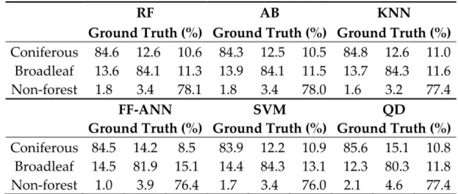
In Table 3, the confusion matrix obtained in the scenario 1 is shown. Almost all classifiers exhibited the highest sensitivity for the non‐forest class, whereas the worst misclassification was between broadleaf and coniferous. This result confirms that L‐band data were more useful to discriminate forest and non‐forest rather than different forest types.

As to scenario 2, whose results are reported in Table 4, the sensitivity was remarkably unbalanced toward the discrimination of forest types for all classifier, whereas they show very poor performance for the non‐forest type. Similar conclusions could be drawn by observing Table 5, where the results for scenario 3 are reported. A noticeable sensitivity balancing was obtained in scenario 4, as reported in Table 6. As to the forest type, four classifiers out of six exhibited sensitivity greater than 80% for both classes, whereas it ranged between 70% and 80% for the non‐forest class. This trend was also observed in the scenario 5 (see Table 7), even though the sensitivity values were slightly lower (about less 1%–2%). The joint use of band C‐ and X‐ (scenario 6, Table 8), on the contrary, did not provide enough information to discriminate the non‐forest class and the sensitivity of classifiers drops of about 50%–70% with respect to the previous scenario. In Table 9, the results of scenario 7 are reported. By comparison with scenario 4 (Table 6), no remarkable trend emerged in terms of sensitivity or misclassification rate.

In order to summarize the comparison, the average accuracies computed on the 10 folds, as well as the standard deviations, are reported in Table 10. RF classification achieved the best overall result (83.1 ± 0.1) and led in six out of seven scenarios. AB performed very closely to RF and both classification methods exhibited very low variance in all scenarios. KNN joins RF as to the best overall result, but the former suffered of poorer results in Scenario 2, 3 and 6. Moreover, some of the classifiers trained in the Scenario 2 resulted strongly biased towards forest classes, which was

(14)

reflected in the higher standard deviations of the accuracy. A similar irregular pattern was exhibited by the SVM classifiers. FF‐ANN and QD sub‐optimally scored with respect to the best ones, even though no remarkable variability emerged across different realizations. All classification methods consistently attained their best in the scenario 7, that is, when all available data were used; the second‐ best result was observed for the joint use of L‐ and X‐bands. Furthermore, the accuracies of all classifiers were remarkably above the 36.4% lower bound threshold, which corresponded to the accuracy of the trivial random assignment based on pixels’ prior distribution.

The average computational times of the tested classification methods are reported in Table 11. The computer simulations were carried out in MATLAB R2019b, on an Intel(R) Core(TM) i7‐8700 CPU @ 3.20GHz, 32 GB RAM, operating system Xubuntu 19.04 and exploiting six parallel processing. The time spent for the hyperparameters optimization was included and it varied according to several parameters, such as the i) dimensionality of predictors, ii) separability of classes, iii) number of parameters and the iv) stopping criterion of the optimization routines. It must be pointed out that, despite of a relatively fast training phase, KNN classifiers are more memory and processor intensive during the prediction phase, significantly being the slowest with respect to the other classification methods.

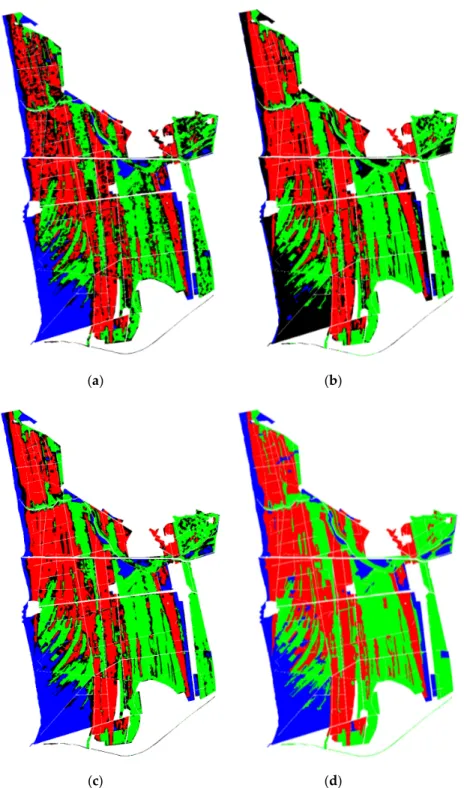
For a visual evaluation, the classification maps obtained with RF are presented in Figure 7, considering three different scenarios. In scenario 1 (Figure 7a), identification between coniferous and broad leaf was scarce, whereas the non‐forest areas were almost correctly identified as blue areas. Conversely, the classification map of scenario 2 (Figure 7b) shows a better discrimination between coniferous (red areas) and broadleaf (green) forests. In scenario 4 (Figure 7c), the improvement in the classification result combining L‐ and X‐ band was clear. Table 3. Confusion matrices in the scenario 1 (PALSAR HH + PALSAR HV) for the classes coniferous, broadleaf and non‐forest areas. RF AB KNN

Ground Truth (%) Ground Truth (%) Ground Truth (%) Coniferous 71.9 25.9 8.8 72.2 26.2 8.7 68.8 27.6 9.0

Broadleaf 25.9 70.2 13.3 25.6 70.0 13.3 28.4 68.0 14.4 Non‐forest 2.2 3.9 78.0 2.2 3.9 78.0 2.7 4.4 76.6

FF‐ANN SVM QD

Ground Truth (%) Ground Truth (%) Ground Truth (%) Coniferous 72.8 27.9 6.0 71.0 26.1 6.8 77.1 38.1 6.2 Broadleaf 25.6 67.7 16.4 27.3 70.7 17.5 19.7 56.7 13.1 Non‐forest 1.6 4.4 77.5 1.7 3.2 75.7 3.2 5.3 80.7 Table 4. Confusion matrices in the scenario 2 (CSK2 HH) for the classes coniferous, broadleaf and non‐forest area. RF AB KNN

Ground Truth (%) Ground Truth (%) Ground Truth (%) Coniferous 83.3 14.7 59.8 82.9 14.4 59.4 62.0 13.1 49.7 Broadleaf 15.4 85.2 30.1 15.7 85.5 30.5 12.3 63.7 23.0 Non‐forest 1.3 0.1 10.0 1.4 0.1 10.2 25.7 23.2 27.3

(15)

Table 5. Confusion matrices in the scenario 3 (ASAR VV) for the classes coniferous, broadleaf and

non‐forest area.

RF AB KNN

Ground Truth (%) Ground Truth (%) Ground Truth (%) Coniferous 81.6 14.8 58.2 83.2 16.5 59.7 82.2 15.4 58.8 Broadleaf 18.4 84.0 36.8 16.8 83.5 40.3 17.8 84.1 38.1 Non‐forest 0.0 1.1 4.9 0.0 0.0 0.0 0.0 0.4 3.1 Table 6. Confusion matrices in the scenario 4 (PALSAR HH + PALSAR HV + CSK2 HH) for the classes coniferous, broadleaf and non‐forest area. RF AB KNN

Ground Truth (%) Ground Truth (%) Ground Truth (%) Coniferous 83.0 13.8 8.5 84.2 13.7 11.1 86.1 17.1 9.9 Broadleaf 16.0 82.2 15.6 14.2 83.0 14.2 11.2 78.4 11.2 Non‐forest 1.0 4.1 75.9 1.6 3.4 74.7 2.7 4.4 78.8 Table 7. Confusion matrices in the scenario 5 (PALSAR HH + PALSAR HV + ASAR VV) for the classes coniferous, broadleaf and non‐forest area. RF AB KNN

Ground Truth (%) Ground Truth (%) Ground Truth (%) Coniferous 81.0 14.6 8.4 80.4 12.8 10.6 82.3 15.5 9.9

Broadleaf 17.7 81.9 16.2 17.6 83.7 12.7 14.9 80.1 10.8 Non‐forest 1.3 3.5 75.4 2.0 3.5 76.6 2.8 4.4 79.4

(16)

Table 8. Confusion matrices in the scenario 6 (CSK2 + ASAR VV) for the classes coniferous, broadleaf

and non‐forest area.

RF AB KNN

Ground Truth (%) Ground Truth (%) Ground Truth (%) Coniferous 79.0 12.8 43.1 85.6 15.0 60.8 85.0 14.8 55.2 Broadleaf 20.1 86.0 36.2 13.4 81.9 29.4 13.3 83.1 23.8 Non‐forest 0.9 1.2 20.7 0.9 3.1 9.8 1.7 2.1 21.0 Table 9. Confusion matrices in the scenario 7 (the PALSAR HH + PALSAR HV + CSK2 + ASAR VV) for the classes coniferous, broadleaf and non‐forest area. RF AB KNN

_{Ground Truth (%) Ground Truth (%) Ground Truth (%)} Coniferous 84.5 14.2 8.5 83.9 12.2 10.9 85.6 15.1 10.8 Broadleaf 14.5 81.9 15.1 14.4 84.3 13.1 12.3 80.3 11.8 Non‐forest 1.0 3.9 76.4 1.7 3.4 76.0 2.1 4.6 77.4

Table 10. Average and standard deviation of the accuracy of the classifiers for each tested scenario

(abbreviations are used for sake of clarity). The best values for scenario are highlighted in bold.

Scenario RF AB KNN FF‐ANN SVM QD

PALSAR 72.3 ± 0.1 72.4 ± 0.1 70.0 ± 0.3 71.6 ± 0.1 71.8 ± 0.1 69.4 ± 0.6 CSK2 70.0 ± 0.0 70.0 ± 0.1 56.0 ± 19.8 68.9 ± 0.1 52.6 ± 21.8 69.3 ± 0.1 ASAR 67.8 ± 0.0 67.8 ± 0.0 57.9 ± 3.3 67.8 ± 0.0 67.3 ± 0.0 67.8 ± 0.0 PALSAR + CSK2 82.3 ± 0.1 82.2 ± 0.1 82.1 ± 0.1 81.3 ± 0.1 81.8 ± 0.0 81.5 ± 0.1 PALSAR + ASAR 81.4 ± 0.1 81.3 ± 0.1 81.1 ± 0.1 80.3 ± 0.1 81.1 ± 0.0 80.8 ± 0.1 CSK2 + ASAR 72.6 ± 0.1 72.6 ± 0.0 69.3 ± 0.2 70.7 ± 0.2 69.5 ± 3.6 71.9 ± 0.1 PALSAR + CSK2 + ASAR 83.1 ± 0.1 83.0 ± 0.1 83.1 ± 0.1 81.9 ± 0.1 82.5 ± 0.0 81.8 ± 0.1

(17)

(a) (b)

(c) (d)

Figure 7. Classification maps of San Rossore test site obtained with random forest by using (a)

PALSAR HH + PALSAR HV; (b) CSK HH and (c) PALSAR HH + PALSAR HV + CSK HH. (d) Reference forest classification map produced by DREAM [27]. Legend: Red: coniferous (correctly classified), Green: broadleaf (correctly classified), Blue: non‐forest (correctly classified), Black: misclassified.

(18)

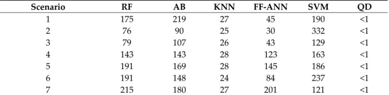
Table 11. Average computational times (s) of the training phase for different classification methods,

including the hyperparameters optimization, as a function of the Scenario. Six parallel processing was used.

Scenario RF AB KNN FF‐ANN SVM QD

1 175 219 27 45 190 <1 2 76 90 25 30 332 <1 3 79 107 26 43 129 <1 4 143 143 28 123 163 <1 5 191 169 28 145 186 <1 6 191 148 24 84 237 <1 7 215 180 27 201 121 <1 5. Discussion

The current study addressed this issue by performing a multi‐step data analysis of forest parameters in a forest area of Central Italy (San Rossore) representative of Mediterranean conditions. The investigation was performed using a consistent dataset of SAR images at L‐ and X‐ bands collected by ALOS/PALSAR, ENVISAT/ASAR and Cosmo‐SkyMed satellites. These images, characterized by different frequencies and polarizations, were used to verify the capability of SAR in mapping forest areas and for discriminating main forest types (coniferous vs. broadleaved).

The results obtained by applying several classifiers confirmed that also in Mediterranean areas the backscattering coefficient at L‐band was generally more indicated than C‐ and X‐ bands to identify forest areas and to separate them for other land covers. On the other hand, the backscattering coefficient at X‐band in HH polarization proved to be more sensitive to forest type and useful to separate broadleaved from coniferous. Moreover, a performance gain in terms of both forest and non‐ forest areas discrimination and coniferous and broadleaf classification inside forested areas was achieved by jointly using L‐ and X‐bands, reaching an overall accuracy greater than 81% for all classifiers. C‐band backscatter, due to the intermediate penetration inside forest canopy, is more affected by the conditions of crowns and to the absence/presence of leaves; it conversely provides scarce contribution to the classification purposes.

An evaluation of classifiers performance should also consider the spatial distribution of the misclassification errors. For instance, by visual inspection of Figure 7c, it emerged that misclassified pixels (i.e., black areas) were mainly clustered along the transition zones from a class to another. As an example, if only edge pixels were considered for validation, the single‐realization accuracy of RF in the case of the joint use of L‐ and X‐bands (scenario 4) would drop from 82.3% to 63.7%. In this specific example, an edge pixel is defined as a pixel that is 8‐connected to a pixel of another class. Thus, it is interesting to compare how different classifiers perform on edge pixels.

In Figure 8a, the unnormalized empirical probability density function of the number of classifiers (on a single realization) making a wrong decision on an edge pixel, given that at least one classifier makes the wrong decision, is reported. The mode of the distribution is strongly polarized on the last bin, indicating that all classifiers tended to wrongly decide on the same edge pixels; more precisely, it can be stated that if some classifier makes a wrong prediction on an edge pixel, then the most probable event is that all classifiers misclassify that pixel. A further quantification of this phenomenon was deduced by observing the empirical cumulative density function in Figure 8b. It could be concluded that all classifiers made the wrong prediction about 50% of the times that an edge pixel was misclassified.

(19)

(a) (b)

Figure 8. Number of classifiers making a wrong prediction on an edge pixel, given that at least one

classifier makes the wrong prediction: (a) unnormalized empirical probability density function and (b) cumulative density function.

Similar performance degradations were observed in all the tested scenarios. Indeed, misclassification on edge pixels is due to several reasons: i) edges sensibility to finite resolution of both ground truth and SAR imagery with respect to inner areas; ii) discrepancy of the ground truth map with respect to the actual ground truth at the date of sensing; iii) blurring due to SAR imagery preprocessing (e.g., multi‐looking, registration); iv) blurring introduced by the despeckling filter. A possible strategy to limit the edge misclassification is to detect edge pixels (e.g., by means of a preliminary segmentation of the image) and discard them. Alternatively, a weight could be assigned to each pixel to measure the reliability of the prediction according to the distance of between a pixel and the closest edge. Integration of information coming from other sensors or computation of spatial features over the SAR imagery itself can be also adopted. Nevertheless, this investigation was beyond the scope of this work and it might be hopefully elaborated in a future work. 6. Conclusions The application of multi‐frequency SAR images to the study of heterogeneous Mediterranean forests, which have not been so far extensively investigated by using microwave remote sensing methods, have been adopted. The role of L‐, C‐ and X‐bands in land classification has been analyzed by applying several machine learning classification methods to data coming from different combinations of sensors and polarization. The joint use of multi‐frequency and multi‐polarization SAR data was shown to improve the classification of heterogeneous Mediterranean forests, allowing the separation of forest areas from non‐forest ones, as well as the identification of broadleaf and coniferous classes inside the forest class. The overall accuracy exceeded 80% when integrating both L‐ and X‐band contributions for almost all considered classifiers; instead, it was significantly lower when considering separately L‐ and X‐band. Furthermore, more homogeneous sensitivity across bands was achieved in the former case. By comparison, the contribution of C‐band had emerged to be of secondary importance.

Random forest classification and support vector machines are two popular classification methods that were tested among others. In our results, the former had shown the best accuracy for all almost the considered scenarios and it was confirmed a powerful tool for classification purposes. The latter, on the contrary, was shown to suffer of unbalanced sensitivity among classes in some scenarios; this behavior could be also motived by the consistent number of hyperparameters that must be tuned to achieve optimality, which is an intrinsic limit of this algorithm with respect to random forest.

This research could be also interesting in view of the OptiSAR Constellation mission, devoted to the Earth surface observation by means of spaceborne optical, L‐ and X‐band SAR sensors, with the aim of developing consistent applications in environmental, hazard and safety monitoring.

(20)

Further test and validation of the presented methodology should be advisable by extending the investigation to other datasets and test areas. Moreover, a supplemental study considering the seasonality of the sensed areas was advisable. Finally, the delineation of ad‐hoc strategies to deal with the classification of forest edge areas is expected to decrease the misclassification error. Author Contributions: conceptualization, A.L. and G.F.; methodology, G.F.; software, A.L. and S.Pe.; validation, S.Pa.; investigation, E.S.; resources, A.G.; data curation, S.Pe.; writing—original draft preparation, A.G. and S.Pe.; writing—review and editing, A.L. and G.F.; supervision, E.S. and S.Pa.; project administration, S.Pa.; funding acquisition, S.Pa.. All authors have read and agreed to the published version of the manuscript. Funding: This research received no external funding.

Acknowledgments: Italian Space Agency (ASI) partially supported this research by providing the Cosmo‐

SkyMed images of the test areas through the ‘SAR for Biomap’ project. The ALOS/PALSAR images were provided under the AO project by JAXA (PI PIGM111T), whereas the ENVISAT/ASAR images were provided by ESA under the Category‐1 proposal “SAR for Biomap” (Project id 28510). The authors wish to warmly thank Drs. Fabio Maselli,Marta Chiesi and Prof. Gherardo Chirici their support and useful comments and suggestions, as well as the Ente Parco Regionale Migliarino and the Comando Stazione Forestale S. Rossore Loc. Cascine Nuove for providing ground truth data of the San Rossore area.

Conflicts of Interest: The authors declare no conflict of interest.

References

1. Waring, R.H.; Running, S.W. Carbon Cycle. In Forest Ecosystems; Academic Press: San Diego, CA, USA, 2007; pp. 59–98, ISBN 978‐0‐12‐370605‐8.

2. McRoberts, R.E. Using satellite imagery and the k‐nearest neighbors technique as a bridge between strategic and management forest inventories. Remote Sens. Environ. 2008, 112, 2212–2221.

3. Guyot, G.; Guyon, D.; Riom, J. Factors affecting the spectral response of forest canopies: A review. Geocarto

Int. 1989, 4, 3–18.

4. Tucker, C.J. Red and photographic infrared linear combinations for monitoring vegetation. Remote Sens.

Environ. 1979, 8, 127–150.

5. Ulaby, F.T.; Dobson, M.C. Handbook of Radar Scattering Statistics for Terrain; The Artech House Remote Sensing Library; Artech House: Norwood, MA, USA, 1989; ISBN 978‐0‐89006‐336‐1.

6. Ulaby, F.T.; Whitt, M.W.; Dobson, M.C. Measuring the propagation properties of a forest canopy using a polarimetric scatterometer. IEEE Trans. Antennas Propagat. 1990, 38, 251–258.

7. Hoekman, D.H. Radar signature and forest vegetation. In Land Observation by Remote Sensing: Theory and

Applications; Buiten, H.J., Clevers, J.G.P.W., Eds.; Current topics in remote sensing; Gordon and Breach

Science Publishers: Yverdon, Switzerland; Langhorne, PA, USA, 1993; pp. 219–235, ISBN 978‐2‐88124‐939‐ 6.

8. Paloscia, S.; Macelloni, G.; Pampaloni, P.; Sigismondi, S. The potential of C‐ and L‐band SAR in estimating vegetation biomass: The ERS‐1 and JERS‐1 experiments. IEEE Trans. Geosci. Remote Sens. 1999, 37, 2107– 2110.

9. Le Toan, T.; Laur, H.; Mougin, E.; Lopes, A. Multitemporal and dual‐polarization observations of agricultural vegetation covers by X‐band SAR images. IEEE Trans. Geosci. Remote Sens. 1989, 27, 709–718. 10. Ferrazzoli, P.; Paloscia, S.; Pampaloni, P.; Schiavon, G.; Sigismondi, S.; Solimini, D. The potential of

multifrequency polarimetric SAR in assessing agricultural and arboreous biomass. IEEE Trans. Geosci.

Remote Sens. 1997, 35, 5–17.

11. Kasischke, E.S.; Melack, J.M.; Craig Dobson, M. The use of imaging radars for ecological applications—A review. Remote Sens. Environ. 1997, 59, 141–156.

12. Ackermann, N.; Thiel, C.; Borgeaud, M.; Schmullius, C. Cosmo‐SkyMed backscatter intensity and interferometric coherence signatures over Germany’s low mountain range forested areas. In Proceedings of the 2012 IEEE International Geoscience and Remote Sensing Symposium, Munich, Germany, 22–27 July 2012; pp. 5514–5517.

13. Le Toan, T.; Beaudoin, A.; Riom, J.; Guyon, D. Relating forest biomass to SAR data. IEEE Trans. Geosci.

Remote Sens. 1992, 30, 403–411.

14. Saatchi, S.; Marlier, M.; Chazdon, R.L.; Clark, D.B.; Russell, A.E. Impact of spatial variability of tropical forest structure on radar estimation of aboveground biomass. Remote Sens. Environ. 2011, 115, 2836–2849.

(21)

15. Woodhouse, I.H.; Mitchard, E.T.A.; Brolly, M.; Maniatis, D.; Ryan, C.M. Radar backscatter is not a “direct measure” of forest biomass. Nat. Clim. Chang. 2012, 2, 556–557.

16. Baghdadi, N.; Le Maire, G.; Bailly, J.S.; Ose, K.; Nouvellon, Y.; Zribi, M.; Lemos, C.; Hakamada, R. Evaluation of ALOS/PALSAR L‐Band Data for the Estimation of Eucalyptus Plantations Aboveground Biomass in Brazil. IEEE J. Sel. Top. Appl. Earth Obs. Remote Sens. 2015, 8, 3802–3811.

17. Santoro, M.; Eriksson, L.; Askne, J.; Schmullius, C. Assessment of stand‐wise stem volume retrieval in boreal forest from JERS‐1 L‐band SAR backscatter. Int. J. Remote Sens. 2006, 27, 3425–3454. 18. Santoro, M.; Askne, J.; Beer, C.; Cartus, O.; Schmullius, C.; Wegmuller, U.; Wiesmann, A. Automatic Model Inversion of Multi‐Temporal C‐band Coherence and Backscatter Measurements for Forest Stem Volume Retrieval. In Proceedings of the IGARSS 2008—2008 IEEE International Geoscience and Remote Sensing Symposium, Boston, MA, USA, 7–11 July2008; p. V‐124. 19. Grover, K.; Quegan, S.; da Costa Freitas, C. Quantitative estimation of tropical forest cover by SAR. IEEE Trans. Geosci. Remote Sens. 1999, 37, 479–490.

20. Santos, J. Airborne P‐band SAR applied to the aboveground biomass studies in the Brazilian tropical rainforest. Remote Sens. Environ. 2003, 87, 482–493.

21. Deutscher, J.; Perko, R.; Gutjahr, K.; Hirschmugl, M.; Schardt, M. Mapping Tropical Rainforest Canopy Disturbances in 3D by COSMO‐SkyMed Spotlight InSAR‐Stereo Data to Detect Areas of Forest Degradation. Remote Sens. 2013, 5, 648–663.

22. Perko, R.; Raggam, H.; Deutscher, J.; Gutjahr, K.; Schardt, M. Forest Assessment Using High Resolution SAR Data in X‐Band. Remote Sens. 2011, 3, 792–815.

23. Scarascia‐Mugnozza, G.; Oswald, H.; Piussi, P.; Radoglou, K. Forests of the Mediterranean region: Gaps in knowledge and research needs. For. Ecol. Manag. 2000, 132, 97–109.

24. Mitchell, A.L.; Tapley, I.; Milne, A.K.; Williams, M.L.; Zhou, Z.S.; Lehmann, E.; Caccetta, P.; Lowell, K.; Held, A. C‐ and L‐band SAR interoperability: Filling the gaps in continuous forest cover mapping in Tasmania. Remote Sens. Environ. 2014, 155, 58–68.

25. Minchella, A.; Del Frate, F.; Capogna, F.; Anselmi, S.; Manes, F. Use of multitemporal SAR data for monitoring vegetation recovery of Mediterranean burned areas. Remote Sens. Environ. 2009, 113, 588–597. 26. Tanase, M.; de la Riva, J.; Santoro, M.; Pérez‐Cabello, F.; Kasischke, E. Sensitivity of SAR data to post‐fire

forest regrowth in Mediterranean and boreal forests. Remote Sens. Environ. 2011, 115, 2075–2085.

27. DREAM. Tenuta di San Rossore; Note illustrative della carta forestale e della fruizione turistica; D.R.E.Am. Italia Soc. Coop. Agr., Poppi, Italy; 2003.

28. Corona, P.; Chirici, G.; Marchetti, M. Forest ecosystem inventory and monitoring as a framework for terrestrial natural renewable resource survey programmes. Plant Biosyst. Int. J. Deal. All Asp. Plant Biol. 2002, 136, 69–82. 29. Richards, J.A. Remote Sensing Digital Image Analysis; Springer: Berlin/Heidelberg, Germany, 2013; ISBN 978‐ 3‐642‐30061‐5. 30. Ferrazzoli, P.; Guerriero, L. Radar sensitivity to tree geometry and woody volume: A model analysis. IEEE Trans. Geosci. Remote Sens. 1995, 33, 360–371.

31. Santi, E.; Paloscia, S.; Pettinato, S.; Fontanelli, G.; Mura, M.; Zolli, C.; Maselli, F.; Chiesi, M.; Bottai, L.; Chirici, G. The potential of multifrequency SAR images for estimating forest biomass in Mediterranean areas. Remote Sens. Environ. 2017, 200, 63–73.

32. Bamler, R.; Hartl, P. Synthetic aperture radar interferometry. Inverse Probl. 1998, 14, R1.

33. Argenti, F.; Lapini, A.; Bianchi, T.; Alparone, L. A Tutorial on Speckle Reduction in Synthetic Aperture Radar Images. IEEE Geosci. Remote Sens. Mag. 2013, 1, 6–35.

34. Breiman, L. Random Forests. Mach. Learn. 2001, 45, 5–32.

35. Quinlan, J.R. Combining Instance‐based and Model‐based Learning. In Proceedings of the Tenth International Conference on International Conference on Machine Learning, Amherst, MA, USA, 27–29 June 1993; Morgan Kaufmann Publishers Inc.: San Francisco, CA, USA, 1993; pp. 236–243. 36. Pal, M. Random forest classifier for remote sensing classification. Int. J. Remote Sens. 2005, 26, 217–222. 37. Camargo, F.F.; Sano, E.E.; Almeida, C.M.; Mura, J.C.; Almeida, T. A Comparative Assessment of Machine‐ Learning Techniques for Land Use and Land Cover Classification of the Brazilian Tropical Savanna Using ALOS‐2/PALSAR‐2 Polarimetric Images. Remote Sens. 2019, 11, 1600. 38. Yu, Y.; Li, M.; Fu, Y. Forest type identification by random forest classification combined with SPOT and multitemporal SAR data. J. For. Res. 2018, 29, 1407–1414.