Scientific Report
DOI: 10.21570/EDGG.PG.44.26-47
GrassPlot v. 2.00 – first update on the database of
multi-scale plant diversity in Palaearctic grasslands
1
Department of Plant Biology and Ecology, University of the Basque Coun-try UPV/EHU, P.O. Box 644, 48080 Bilbao, Spain; [email protected]; itzia r.g a rcia@ eh u. es, ma rcen o.corra d o@gma il. com, j [email protected]
2Department of Environmental Biology, Sapienza University of Rome, P.le Aldo Moro 5, 00185 Rome, Italy; [email protected] 3
Botanical Garden Center for Biological Diversity Conservation in Powsin, Polish Academy of Sciences, Prawdziwka St. 2, 02-973 Warsaw, Poland; [email protected],[email protected],[email protected] 4
Department of Plant Ecology and Environmental Conservation, Faculty of Biology, University of Warsaw, ul. Żwirki i Wigury 101, 02-089 Warsaw, Poland; [email protected]
5
Vegetation Ecology Group, Institute of Natural Resource Sciences (IUNR), Zurich University of Applied Sciences (ZHAW), Grüentalstr. 14, 8820 Wä-denswil, Switzerland; [email protected], [email protected], [email protected],[email protected]
6Department STEBICEF, Botanical Unit, University of Palermo, via Archiarafi 38, 90123 Palermo, Italy; [email protected]
7Department of Landscape Monitoring, Norwegian Institute of Bioeconomy Research, Holtvegen 66, 9269 Tromsø, Norway; [email protected] 8
Department of Forest Biodiversity, Faculty of Forestry, University of Agri-culture in Kraków, al. 29 Listopada 46, 31-425 Kraków, Poland; [email protected]
9
Department of Biological Sciences, University of Alberta, Edmonton, AB, T6G 2R3, Canada;[email protected]
10Department of Plant and Fungal Diversity and Resources, Institute of Biodiversity and Ecosystem Research, Bulgarian Academy of Sciences, Acad. G. Bonchev, bl. 23, 1113 Sofia, Bulgaria; [email protected] 11Department Computational Landscape Ecology, Helmholtz Centre for Environmental Research - UFZ, Permoserstraße 15, 04318 Leipzig, Ger-many; [email protected], [email protected]
12
German Centre for Integrative Biodiversity Research (iDiv) Halle-Jena-Leipzig, Deutscher Platz 5e, 04103 Halle-Jena-Leipzig, Germany
13Department of Botany and Zoology, Faculty of Science, Masaryk Univer-sity, Kotlářská 2, 61137 Brno, Czech Republic; [email protected], p a v e l . d r e v o j a n @ s e z n a m . c z, h a j e k @ s c i . m u n i . c z, [email protected], [email protected]
14
Institute of Biology, University of Opole, Oleska St., 45-052 Opole, Poland 15Biodiversity & Conservation Biology, WSL Swiss Federal Research Insti-tute, Zürcherstrasse 111, 8903 Birmensdorf, Switzerland; [email protected], [email protected], [email protected] 16Department of Botany and Soroksár Botanical Garden, Faculty of Horti-cultural Science, Szent István University, Villány Street 29-43, 1118 Buda-pest, Hungary; [email protected]
17Department of Biological Sciences, University of Bergen, Postbox 7803, 5020 Bergen, Norway; [email protected],[email protected]
18Department of Botany, University of Innsbruck, Sternwartestr. 15, 6020 Innsbruck, Austria; [email protected]
19
Research Unit of Biodiversity (CSIC, UO, PA), Oviedo University, Campus de Mieres, 33600 Mieres, Spain; [email protected] 20Botanical Garden, University of Wrocław, Sienkiewicza 23, 50-335 Wro-cław, Poland; [email protected], [email protected] 21 Geobotany and Ecology Department, M.G. Kholodny Institute of Botany NAS of Ukraine, Tereschenkivska str. 2, 1601 Kyiv, Ukraine; [email protected]
22Institute of Botany and Landscape Ecology, Greifswald University, Sold-mannstr. 15, 17487 Greifswald, Germany; [email protected] 23
Division of Forest, Nature and Landscape, Department of Earth and Envi-ronmental Sciences, KU Leuven, Celestijnenlaan 200e, 3001 Leuven, Bel-gium; [email protected]
24
Agroforestry Engineering Area, Department of Organisms and Systems Biology, Polytechnic School of Mieres, Oviedo University, Gonzalo Gutiérrez de Quirós s/n, 33600 Mieres, Asturias, Spain; [email protected]
Idoia Biurrun
1*, Sabina Burrascano
2, Iwona Dembicz
3,4,5, Riccardo Guarino
6, Jutta Kapfer
7, Remigiusz
Pielech
8, Itziar Garcia-Mijangos
1, Viktoria Wagner
9, Salza Palpurina
10, Anne Mimet
11,12, Vincent
Pellissier
11, Corrado Marcenò
1,13, Arkadiusz Nowak
3,14,
Ariel Bergamini
15, Steffen Boch
15, Anna Mária
Csergő
16, John-Arvid Grytnes
17, Juan Antonio Campos
1,
Brigitta Erschbamer
18, Borja Jiménez-Alfaro
19,
Zygmunt Kącki
20, Anna Kuzemko
13,21,
Michael Manthey
22,
Koenraad van Meerbeek
23,
Grzegorz
Swacha
21, Elias Afif
24, Juha M. Alatalo
25,26, Michele Aleffi
27, Manuel Babbi
5, Zoltán Bátori
28, Elena
Belonovskaya
29, Christian Berg
30, Kuber Prasad Bhatta
17, Laura Cancellieri
31, Tobias Ceulemans
32, Balázs
Deák
33, László Demeter
34,
Lei Deng
35, Jiří Doležal
36, Christian Dolnik
37, Wenche Dramstad
38, Pavel
Dřevojan
13, Klaus Ecker
15, Franz Essl
39, Jonathan Etzold
40, Goffredo Filibeck
31, Wendy Fjellstad
38, Behlül
Güler
41, Michal Hájek
13, Daniel Hepenstrick
5, John G. Hodgson
42, João P. Honrado
43, Annika K.
Jägerbrand
44, Monika Janišová
45, Philippe Jeanneret
46, András Kelemen
47, Philipp Kirschner
48, Ewelina
Klichowska
49, Ganna Kolomiiets
50, Łukasz Kozub
4, Jan Lepš
36, Regina Lindborg
51, Swantje Löbel
52,
Angela Lomba
43, Martin Magnes
30, Helmut Mayrhofer
30, Marek Malicki
53, Ermin Mašić
54, Eliane S.
Meier
46, Denis Mirin
55, Ulf Molau
56, Ivan Moysiyenko
57, Alireza Naqinezhad
58, Josep M. Ninot
59,
Marcin Nobis
49, Christian Pedersen
38, Aaron Pérez-Haase
59,60, Jan Peters
61, Eulàlia Pladevall-Izard
59, Jan
Roleček
13,62, Vladimir Ronkin
63, Galina Savchenko
63, Dariia Shyriaieva
18, Hanne Sickel
38, Carly Stevens
64,
Sebastian Świerszcz
3, Csaba Tölgyesi
28, Nadezda Tsarevskaya
29, Orsolya Valkó
47, Carmen Van
Mechelen
65, Iuliia Vashenyak
66, Ole Reidar Vetaas
67, Denys Vynokurov
13,18, Emelie Waldén
51, Stefan
25
Department of Biological and Environmental Sciences, Qatar University, 2713 Doha, Qatar; [email protected]
26Environmental Science Center, Qatar University, 2713 Doha, Qatar 27School of Biosciences and Veterinary Medicine, Plant Diversity & Ecosys-tems Management Unit, Bryology Laboratory & Herbarium, University of Camerino, Via Pontoni 5, 62032 Camerino (MC), Italy; [email protected]
28Department of Ecology, University of Szeged, Közép fasor 52, 6726 Szeged, Hungary; [email protected],[email protected]
29
Institute of Geography, Russian Academy of Sciences, Staromonetny per., 29, 119017 Moscow, Russia; [email protected], [email protected]
30
Department of Plant Sciences, Institute of Biology, University of Graz, Holteigasse 6, 8010 Graz, Austria; [email protected], [email protected],[email protected]
31
Department of Agricultural and Forestry Sciences (DAFNE), University of Tuscia, via San Camillo de Lellis snc, 01100 Viterbo, Italy; [email protected], [email protected]
32
Plant Conservation and Population Biology, Department of Biology, KU Leuven, Kasteelpark Arenberg 31 box 2435, 3001 Leuven, Belgium; [email protected]
33MTA-DE Biodiversity and Ecosystem Services Research Group, Hungarian Academy of Sciences, Egyetem tér 1, 4032 Debrecen, Hungary; [email protected]
34
State Agency for Protected Areas, pta. Libertatii nr. 5, 530140 Miercurea-Ciuc, Romania; [email protected]
35
State Key Laboratory of Soil Erosion and Dryland Farming on the Loess Plateau, Institute of Soil and Water Conservation, Northwest A&F Univer-sity, NO. 26 Xinong Road, 712100 Yangling, China; [email protected] 36
Department of Botany, Faculty of Science, University of South Bohemia, Branisovska 31, 370 05 Ceske Budejovice, Czech Republic; [email protected],[email protected]
37
Ecology Centre Kiel, Kiel University, Olshausenstr. 40, 24098 Kiel, Ger-many; [email protected]
38Department of Landscape Monitoring, Norwegian Institute of Bioecon-omy Research, P.O. Box 115, 1431 Ås, Norway; [email protected], [email protected], [email protected], [email protected]
39
Division of Conservation Biology, Vegetation and Landscape Ecology, Department of Botany and Biodiversity Research, University of Vienna, Rennweg 14, 1030 Vienna, Austria; [email protected]
40ESTOK UG, Elbestr. 97, 16321 Bernau (bei Berlin), Germany; [email protected]
41
Biology Education, Dokuz Eylul University, Uğur Mumcu Str. 135. No: 5, 35380 Buca, İzmir, Turkey; [email protected]
42Animal and Plant Sciences Sheffield University, Alfred Denny Building, Western Bank, S10 2TN Sheffield, United Kingdom; [email protected]
43Research Centre in Biodiversity and Genetic Resources (CIBIO) - Research Network in Biodiversity and Evolutionary Biology (InBIO), University of Porto, Campus Agrário de Vairão, Rua Padre Armando Quintas, nº 7, 4485-641 Vairão, Vila do Conde, Portugal; [email protected], [email protected]
44Department of Construction Engineering and Lighting Science, School of Engineering, Jönköping University, P. O. Box 1026, 551 11, Jönköping, Swe-den; [email protected]
45Institute of Botany, Plant Science and Biodiversity Center, Slovak Acad-emy of Sciences, Ďumbierska 1, 974 11 Banská Bystrica, Slovakia; [email protected]
46Research Division Agroecology and Environment, Agroscope, Reckenhol-z s t r a s s e 1 9 1 , 8 0 4 6 Z ü r i c h , S w i t z e r l a n d ; p h i l [email protected],[email protected]
47
MTA-DE Lendület Seed Ecology Research Group, Hungarian Academy of Sciences, Egyetem tér 1, 4032 Debrecen, Hungary; [email protected], [email protected]
48Naturpark Kaunergrat Pitztal - Fließ – Kaunertal, Gachenblick 100, 6251 Fließ, Austria; [email protected]
49Institute of Botany, Jagiellonian University, Gronostajowa 3, 30-387 Kraków, Poland; [email protected], [email protected], [email protected]
50National Nature Park "Buzky Gard", 85, Pervomaiska str., 55223 Mygyia, Mykolaiv region Ukraine; [email protected]
51Dept. of Physical Geography, Stockholm University, 106 91 Stockholm, Sweden; [email protected], [email protected] 52
Landscape Ecology and Environmental Systems Analysis, Institute of Geoecology, TU Braunschweig, Langer Kamp 19c, 38106 Braunschweig, Germany; [email protected]
53
Department of Botany, University of Wrocław, ul. Kanonia 6/8, 50-328 Wrocław, Poland; [email protected]
54Department of Biology, Faculty of Science, University of Sarajevo, Zmaja od Bosne 33-35, 71000 Sarajevo, Bosnia and Herzgovina; [email protected]
55Department of Vegetation Science and Plant Ecology, Biological faculty, St. Petersburg State University, Universitetskaja emb., 7/9, 199034 Saint Petersburg, Russia; [email protected]
56
Department of Biological and Environmental Sciences, University of Goth-enburg, P.O. Box 461, 405 30 Gothenburg, Sweden; [email protected]
57
Department of Botany, Kherson State University, Universytetska St. 27, 73000 Kherson, Ukraine; [email protected]
58Department of Biology, Faculty of Basic Sciences, University of Mazanda-ran, P.O. Box 47416-95447, Babolsar, Iran; [email protected] 59Department of Evolutionary Biology, Ecology and Environmental Sciences, Universitat de Barcelona, Av. Diagonal 643, 08028 Barcelona, Spain; [email protected], [email protected], [email protected] 60Department of Biosciences, University of Vic, Carrer de la Laura 13, 08500 Vic, Spain
61
Michael-Succow-Foundation, Ellernholzstr. 1/3, 17489 Greifswald, Ger-many; [email protected]
62
Department of Vegetation Ecology, Institute of Botany, Czech Academy of Sciences, Lidická 25/27, 60200 Brno, Czech Republic
63Department of Zoology and Animal Ecology, V.N. Karazin Kharkiv National University, 4 Svobody Sq, 61022 Kharkiv, Ukraine; [email protected], [email protected]
64Lancaster Environment Centre, Lancaster University, LA1 4YQ Lancaster, United Kingdom; [email protected]
65PXL Bio-Research, PXL University College, Agoralaan H, 3590 Diepenbeek, Belgium; [email protected]
66
Vasul’ Stus Donetsk National University, 600th Anniversary Street, 21021, Vinnytsia, Ukraine; [email protected]
67Department of Geography, University of Bergen, Fosswinckelsgate 6, 5020 Bergen, Norway; [email protected]
68Life Science Center Weihenstephan, Technische Universität München, Liesel-Beckmann-Straße 2, 85354, Freising, Germany; [email protected]
69Training Department, Stroyproekt Engineering Group, Dunaisky prospect 13A, 196158, Saint Petersburg, Russia; [email protected]
70
Plant Ecology, Bayreuth Center of Ecology and Environmental Research (BayCEER), University of Bayreuth, Universitätsstr. 30, 95447 Bayreuth, Germany
Introduction
Since 2009, the Eurasian Dry Grassland Group (EDGG) has been conducting Field Workshops in various regions of the Palaearctic realm to collect high-quality multi-scale diversity and composition data of various, mostly dry grassland types (e.g. Turtureanu et al. 2014; Kuzemko et al. 2016; Polyakova et al. 2016; for overview of the sampled data, see Dengler et al. 2016a) following the same sampling methodology (Dengler et al. 2016b). In March 2017, the establishment of the collaborative vegetation-plot database GrassPlot al-lowed merging the data collected by the EDGG with the previously established “Database Species-Area Relation-ships in Palaearctic Grasslands” (Dengler et al. 2012). The resulting GrassPlot database is registered in the Global In-dex of Vegetation-Plot Databases (Dengler et al. 2011) un-der ID EU-00-003 (Dengler et al. 2018) and contains vegeta-tion-plot data of grasslands in the widest sense (i.e. any vegetation type except forests, tall shrublands, aquatic and segetal communities) from the Palaearctic biogeographic realm (i.e. Europe, North Africa, and West, Central, North and Northeast Asia). The focus of GrassPlot is on data of precisely delimited plots, both multi-grain, nested-plot data of any plot size and single-grain data matching one of eight EDGG standard grain sizes (Dengler et al. 2018).
The purpose of GrassPlot is to provide quality data for broad -scale analyses of various aspects of vegetation diversity. The concept of GrassPlot and the content of its first public version 1.00 have been described by Dengler et al. (2018). Since this publication, GrassPlot data have been intensively used for broad-scale biodiversity analyses, such as species-area relationships (SARs) in continuous vegetation (Dengler et al. 2019), or manuscripts in preparation on small-scale beta diversity, and “benchmarking” Palaearctic grassland diversity. At the same time, the content and functionality of GrassPlot have significantly increased. This paper provides an overview of the improvements in the structure and con-tent of the database since version 1.00.
New functionalities
Addition and harmonization of header data
Information on nestedness. GrassPlot includes both
single-grain data (hereafter individual plots) and nested-plot data consisting of subplots of several grain sizes, often replicated per grain size. All subplots of a nested series are included in one macro plot or mother plot, also with a complete species list (hereafter largest subplot). We have added several bi-nary (Y/N) header data to document different aspects of nestedness: Individual plot, Independent plot (individual plots and largest subplots combined), Belonging to nested series with at least 2 sizes, Belonging to nested series with at least 4 sizes, Belonging to nested series with at least 7 sizes, and Perfect nesting. The latter indicates if the nested series corresponds to a perfect nesting or not, e.g., if all subplots of a certain size are included in the next larger subplot (Fig. 1). The additional column Distorting sizes indicates which are the grain sizes that are impeding the perfect nesting; if these distorting sizes were removed, a perfect nesting would result. Fig. 1 shows schemes of the three main types of nested sampling designs in GrassPlot, two with perfect nesting (Figs. 1a, 1b) and a third one with non-perfect nest-ing (Fig. 1c).
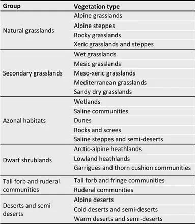
Grassland types and biomes. Data collected in GrassPlot
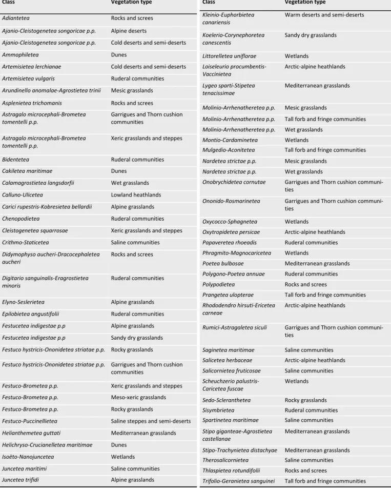
represent different types of grasslands in the broadest sense. To allow future users and projects to deal with this considerable diversity of vegetation, we created a two-level vegetation typology with 22 vegetation types grouped into six broad groups: natural grasslands, secondary grasslands, azonal habitats, dwarf shrublands, tall forb and ruderal communities, and deserts and semi-deserts (Table 1). We also created expert rules to assign phytosociological syntaxa already included in GrassPlot to these 22 vegetation types (Table 2). Vegetation type was assigned based on phytosoci-ological affinity or on other information provided by data Palaearctic Grasslands 44 (2020): 26-47
Abstract: GrassPlot is a collaborative vegetation-plot database organised by the Eurasian Dry Grassland Group (EDGG) and listed in the
Global Index of Vegetation-Plot Databases (GIVD ID EU-00-003). Following a previous Long Database Report (Dengler et al. 2018,
Phyto-coenologia 48, 331–347), we provide here the first update on content and functionality of GrassPlot. The current version (GrassPlot v.
2.00) contains a total of 190,673 plots of different grain sizes across 28,171 independent plots, with 4,654 nested-plot series including at least four grain sizes. The database has improved its content as well as its functionality, including addition and harmonization of header data (land use, information on nestedness, structure and ecology) and preparation of species composition data. Currently, GrassPlot data are intensively used for broad-scale analyses of different aspects of alpha and beta diversity in grassland ecosystems.
Keywords: biodiversity; community ecology; Eurasian Dry Grassland Group (EDGG); Global Index of Vegetation-Plot Databases (GIVD);
grassland vegetation; GrassPlot; macroecology; nested plot; Palaearctic; scale dependence; species-area relationship (SAR); vegetation-plot database.
Abbreviations: EDGG = Eurasian Dry Grassland Group; EVA = European Vegetation Archive; GIVD = Global Index of Vegetation-Plot
Data-bases; GrassPlot = Database of Scale-Dependent Phytodiversity Patterns in Palaearctic Grasslands; SAR = species-area relationship. Submitted: 25 November 2019; first decision: 11 December 2019; accepted: 12 December 2019
Scientific Editor: Frank Yonghong Li Linguistic Editor: Richard Jefferson
Fig. 1. Examples of nested-plot sampling schemes found in the GrassPlot database: a) perfect nesting with four grain sizes, without replication of the subplots; b) perfect nesting with eight grain sizes and replication at smaller grain sizes (field sampling standard with two replicates of each grain size except the largest, which is used during EDGG Field Work-shops; for details see Dengler et al. 2016b), c) non-perfect nesting with eight grain sizes, where the smallest subplots completely tessellate the largest subplot. In this example, a typical GLORIA sampling design is shown (Pauli et al. 2012). Only the smallest subplots and the largest one are actually sampled in the field, while all intermediate subplot sizes are created post hoc by joining species lists of adjacent subplots. To achieve more different grain sizes, we accepted some that did not allow full tessellation of the largest subplot (see grey areas adjacent to subplots of grain sizes 4-7) and thus distorted the perfect nesting. When the distorting sizes of subplots were removed, a perfect nesting would result.
collectors, e.g., vernacular names, species composition, lo-calisation, and so on.
We also assigned each plot both to biomes and to geo-graphic regions. For biomes, we used the recent classifica-tion by Bruelheide et al. (2019, based on Schultz 2005), which recognizes ten terrestrial biomes, all of them occur-ring in the Palaearctic realm, except “Tropics with year-round rain”. We have assigned all plots in GrassPlot to one of these nine biomes using plot coordinates. As a result, all biomes present in the Palaearctic realm except “Tropics with summer rain”, that occurs marginally on the Arabian Peninsula, are represented in GrassPlot. For geographic re-gionalization, we used Törok & Dengler (2018) and Dengler et al. (in press).
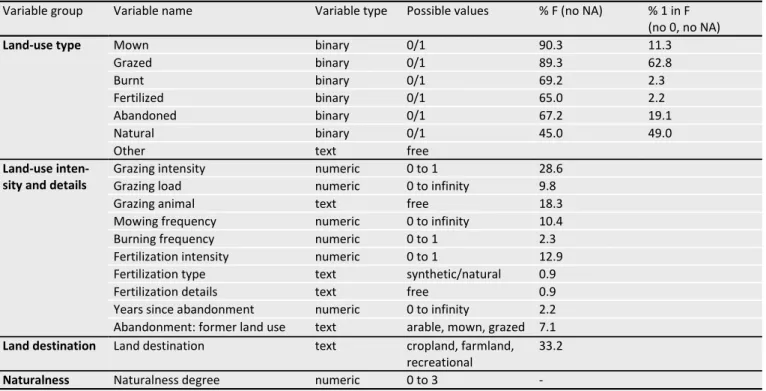
Land-use data. Land use is the main current driver of
biodi-versity change and loss worldwide (Collins et al. 1998). Vegetation survey databases provide spatially explicit infor-mation on local biodiversity (richness and/or composition). However, associated land-use information is generally scarce (but see Niedrist et al. 2009; Hudson et al. 2014). The lack of reliably coupled biodiversity and land-use data at a local scale that is available over large geographic extents substantially impedes our understanding of how biodiver-sity responds to anthropogenic environmental change. The current version of GrassPlot now includes consistent and standardized information on the land use and land-use
intensity of the plots. Information on land-use was provided by data contributors with different degrees of detail. It has been structured into 19 different land-use variables, created to capture as much information as possible from existing datasets. The structure of the land-use data has been devel-oped to meet the needs of future analyses regarding land use-data and to guide future sampling efforts. The 19 land-use variables are structured into four categories: land-land-use type (seven variables), land-use intensity and details (relative to each land-use type), land destination (for what purpose the land is used) and naturalness degree (see Table 3). Each grassland has one or several land-use types (for example it can be mown and fertilized), and a grassland can be mown for different purposes (land destination) such as farming (feeding cattle) or managing a public park (recreational destination). Land destination is a coarse cate-gorisation which is expected to include several types of management practices.
Importantly, all plots of the GrassPlot database (190,673 plots) now have a land-use type, while other land-use vari-ables are not available for all plots, indicated as NA (Table 3). Moreover, the variable Naturalness degree is still under development, and will be added when it is computed.
Environmental and structural data. GrassPlot v. 2.00 has
also notably improved the coverage and consistency of sev-eral environmental and structural header data, which are stored with standardized measurement units. Topographic data are readily and consistently available for many plots with different degrees of coverage, e.g. 88% for Elevation, 34% for Aspect and Inclination, 5% for Microrelief. Microre-lief is defined as the maximum distance to the ground when placing a stick on the ground in the most rugged part of the plot, measured perpendicular to the stick. The soil data with better coverage are pH H20 (15%), Soil texture class (14%),
Conductivity (10%) and Soil depth (10%). Of the structural header data, Tree cover (95%), Shrub cover (50%), Herb cover (49%), Total vegetation cover (39%) and Cryptogam cover (37%) are the variables with better coverage. Addi-tionaly, Litter cover is provided for 31% of plots, Proportion of stones, gravel and fine soil for 21% of plots and Mean height of the herb layer for 13% of plots. All environmental and structural data stored in GrassPlot have been directly measured or estimated in the field, or, in the case of soil parameters, in the laboratory using soil samples collected in the plots. Climatic and more complete topographic data can be retrieved from digital models using plot geographic coor-dinates, but the database is focused on directly measured data. Of course, projects using GrassPlot data may be able to combine them with environmental data extracted from digital models.
Preparation of species composition data
As reported by Dengler et al. (2018), the GrassPlot database also includes species composition data for most datasets (93%). This means that for 90.7% of the plots (Table 4), in addition to species richness data, there is also a complete list of vascular plant species and often also of lichens and
Table 1. Two-level vegetation typology applied in GrassPlot v. 2.00. Since the assignments to the vegetation types and groups were largely based on syntaxonomy, there are some grey zones, e.g. some xeric grasslands might be secondary.
Group Vegetation type
Natural grasslands
Alpine grasslands Alpine steppes Rocky grasslands
Xeric grasslands and steppes
Secondary grasslands
Wet grasslands Mesic grasslands Meso-xeric grasslands Mediterranean grasslands Sandy dry grasslands
Azonal habitats
Wetlands
Saline communities Dunes
Rocks and screes
Saline steppes and semi-deserts
Dwarf shrublands
Arctic-alpine heathlands Lowland heathlands
Garrigues and thorn cushion communities Tall forb and ruderal
communities
Tall forb and fringe communities Ruderal communities
Deserts and semi-deserts
Alpine deserts
Cold deserts and semi-deserts Warm deserts and semi-deserts
Table 2. Assignment rules for phytosociological syntaxa to the 22 vegetation types as defined in GrassPlot v. 2.00, given at class level. Classes occurring in Europe are named after Mucina et al. (2016), classes from outside Europe according to various sources (Ermakov & Krestov 2009; Wehrden et al. 2009; Ermakov et al. 2014; Noroozi et al. 2014; Reinecke et al. 2017; Hüseynova & Yalçin 2018; Nowak et al. 2018). Classes absent in GrassPlot data are not shown in the table. For the classes with the notation p.p., the assignment is made at order or alliance level (not shown here).
Class Vegetation type
Adiantetea Rocks and screes
Ajanio-Cleistogenetea songoricae p.p. Alpine deserts
Ajanio-Cleistogenetea songoricae p.p. Cold deserts and semi-deserts
Ammophiletea Dunes
Artemisietea lerchianae Cold deserts and semi-deserts
Artemisietea vulgaris Ruderal communities
Arundinello anomalae-Agrostietea trinii Mesic grasslands
Asplenietea trichomanis Rocks and screes
Astragalo microcephali-Brometea tomentelli p.p.
Garrigues and Thorn cushion communities
Astragalo microcephali-Brometea tomentelli p.p.
Xeric grasslands and steppes
Bidentetea Ruderal communities
Cakiletea maritimae Dunes
Calamagrostietea langsdorfii Wet grasslands
Calluno-Ulicetea Lowland heathlands
Carici rupestris-Kobresietea bellardii Alpine grasslands
Chenopodietea Ruderal communities
Cleistogenetea squarrosae Xeric grasslands and steppes
Crithmo-Staticetea Saline communities
Didymophyso aucheri-Dracocephaletea aucheri
Rocks and screes
Digitario sanguinalis-Eragrostietea minoris
Ruderal communities
Elyno-Seslerietea Alpine grasslands
Epilobietea angustifolii Ruderal communities
Festucetea indigestae p.p Alpine grasslands
Festucetea indigestae p.p Sandy dry grasslands
Festuco hystricis-Ononidetea striatae p.p. Rocky grasslands
Festuco hystricis-Ononidetea striatae p.p. Garrigues and Thorn cushion communities
Festuco-Brometea p.p. Xeric grasslands and steppes
Festuco-Brometea p.p. Meso-xeric grasslands
Festuco-Brometea p.p. Rocky grasslands
Festuco-Puccinellietea Saline steppes and semi-deserts
Helianthemetea guttati Mediterranean grasslands
Helichryso-Crucianelletea maritimae Dunes
Isoëto-Nanojuncetea Wetlands
Juncetea maritimi Saline communities
Juncetea trifidi Alpine grasslands
Class Vegetation type
Kleinio-Euphorbietea canariensis
Warm deserts and semi-deserts
Koelerio-Corynephoretea canescentis
Sandy dry grasslands
Littorelletea uniflorae Wetlands
Loiseleurio procumbentis-Vaccinietea Arctic-alpine heathlands Lygeo sparti-Stipetea tenacissimae Mediterranean grasslands
Molinio-Arrhenatheretea p.p. Mesic grasslands
Molinio-Arrhenatheretea p.p. Tall forb and fringe communities
Molinio-Arrhenatheretea p.p. Wet grasslands
Montio-Cardaminetea Wetlands
Mulgedio-Aconitetea Tall forb and fringe communities
Nardetea strictae p.p. Mesic grasslands
Nardetea strictae p.p. Wet grasslands
Onobrychidetea cornutae Garrigues and Thorn cushion
communi-ties
Ononido-Rosmarinetea Garrigues and Thorn cushion
communi-ties
Oxycocco-Sphagnetea Wetlands
Oxytropidetea persicae Arctic-alpine heathlands
Papaveretea rhoeadis Ruderal communities
Phragmito-Magnocaricetea Wetlands
Poetea bulbosae Mediterranean grasslands
Polygono-Poetea annuae Ruderal communities
Polypodietea Rocks and screes
Prangetea ulopterae Tall forb and fringe communities
Rhododendro hirsuti-Ericetea carneae
Arctic-alpine heathlands
Rumici-Astragaletea siculi Garrigues and Thorn cushion
communi-ties
Saginetea maritimae Saline communities
Salicetea herbaceae Arctic-alpine heathlands
Salicornietea fruticosae Saline communities
Scheuchzerio palustris-Caricetea fuscae
Wetlands
Sedo-Scleranthetea Rocky grasslands
Sisymbrietea Ruderal communities
Spartinetea maritimae Saline communities
Stipo giganteae-Agrostietea castellanae
Mediterranean grasslands
Stipo-Trachynietea distachyae Mediterranean grasslands
Therosalicornietea Saline communities
Thlaspietea rotundifolii Rocks and screes
bryophytes, either as presence/absence or cover-abundance information. This is the result of the work car-ried out between GrassPlot versions 1.00 and 2.00 to inte-grate the species composition data into a single uniform structure.
Most of the datasets were supplied as species × plot matri-ces (“wide tables”). Since such wide format data are neither suitable for merging into a single dataset nor can be filtered for functional groups or vegetation layers, they were trans-formed into a “long format” (see example in Appendix 1)
using different packages suitable for data manipulation in R (e.g. plyr, dplyr and tidyr) (Wickham et al. 2017; Wickham & Henry 2019). In the long format, each row consists of a spe-cies record, i.e., an occurrence of a spespe-cies in a plot or sub-plot. Additional columns provide information on plant group, vegetation layer, species abundance and abundance-scale. Abundance-scale is a binary column, indicating whether the value in Abundance column is a presence/ absence value (P/A = 0/1) or a cover-abundance value at the percentage scale (cover: 0-100). Cover abundance values
Table 3. Land-use variables in GrassPlot v. 2.00 and the percentage of plots for which the information is available (% F). The percentages refer to the independent plots (N = 28,171). For binary variables, the column “% 1 in F” indicates the percentage frequency of the management technique among the plots that have this land-use information. Some plots have a combined land use (mown and grazed; natural and grazed; etc.), so the sum of plots in each specific land use can exceed the total number of plots in GrassPlot. “NA” indicates missing information.
Variable group Variable name Variable type Possible values % F (no NA) % 1 in F (no 0, no NA)
Land-use type Mown binary 0/1 90.3 11.3
Grazed binary 0/1 89.3 62.8
Burnt binary 0/1 69.2 2.3
Fertilized binary 0/1 65.0 2.2
Abandoned binary 0/1 67.2 19.1
Natural binary 0/1 45.0 49.0
Other text free
Land-use inten-sity and details
Grazing intensity numeric 0 to 1 28.6
Grazing load numeric 0 to infinity 9.8
Grazing animal text free 18.3
Mowing frequency numeric 0 to infinity 10.4
Burning frequency numeric 0 to 1 2.3
Fertilization intensity numeric 0 to 1 12.9 Fertilization type text synthetic/natural 0.9
Fertilization details text free 0.9
Years since abandonment numeric 0 to infinity 2.2 Abandonment: former land use text arable, mown, grazed 7.1
Land destination Land destination text cropland, farmland, recreational
33.2
Naturalness Naturalness degree numeric 0 to 3 -
Table 4. Overview of some key parameters of GrassPlot v. 2.00 covering access regime, methodological aspects and tem-poral and elevational distribution. The column “NA” indicates the fraction of plots in GrassPlot v. 2.00 for which the re-spective field is currently without content. The percentages refer to the independent plots (N = 28,171).
Parameter NA Frequency distribution of parameter values
Availability of data
Access regime < 0.1% 1 – restricted access (12.0%); 2 – semi-restricted access (86.2%); 3 – free access (1.7%) Availability of compositional data – Yes-ready (10.0%); Yes-in preparation (80.7); to be provided later (5.4%); no (3.8%)
Methodological aspects
Recording method 0.2% Shoot presence (69.9%); rooted presence (29.9%)
Plot shape 0.1% Squares (81.6%); rectangles 1:1.6 (0.2%); rectangles more elongated than 1:2 (0.3%); circles (18.0%)
Accuracy of coordinates 0.4% ≤ 1 m (18.3%); 1.1–10 m (47.5%); 11–100 m (12.3%); 101–1,000 m (16.4%); > 1,000 m (5.2%)
Spatio-temporal distribution
Year of recording - Before 1980 (0.1%); 1980–1989 (10.5%); 1990–1999 (13.3%); 2000–2009 (17.7%); 2010 and later (59.3%)
Elevation 12.0% ≤ 10 m a.s.l. (14.9%); 11–100 m a.s.l. (9.2%); 101–1,000 m a.s.l. (28.8%); 1,001–2,000 m a.s.l. (20.1%); 2,001–3,000 m a.s.l. (8.5%); 3,001–4,000 m a.s.l. (3.7%); > 4,000 m a.s.l. (2.8%)
that were originally measured by means of categorical scales (e.g. different variants of Br.-Bl., Londo, and so on) have already been transformed to percentage during the wide data format by choosing the midpoint of the upper and lower boundaries of a cover class. The original cover-abundance scale has been stored in the database together with all other plot-level metadata, plus geographic, environ-mental, land-use and structural data. Species composition long-format tables also maintain relevant metadata such as the GrassPlot ID of the single plot or subplot of a nested-series, the ID of the largest subplot within which the subplot is nested (only for nested-plots) and its grain size. This data structure allows data to be combined within and across datasets for later analyses on species composition either by using the long format or reshaping it into a wide format of species × plot matrices.
While the data are being prepared in a long format, pro-gress is also being made to develop a process to semi-automatically adjust species nomenclature, i.e. correcting typographical errors and homogenizing different levels of identification detail and differences in species name format (e.g. removing authorities from taxon names). This allows taxon names to be standardized according to “The Plant List” (www.theplantlist.org), using the taxonstand package (Cayuela et al. 2012) in R (R Core Team 2019). In addition, we plan to add a column named "determ_qual" to indicate for each taxon its quality of determination: 1 – determined to the species level (e.g. Viola arvensis), 0.5 – determination to species level not certain (e.g. Viola arvensis aggr., Viola cf. arvensis, Viola arvensis/kitaibeliana), 0.2 – species un-known (species epithet missing); 0 – genus unun-known (e.g. Violaceae). This would allow us to calculate a "species com-position quality" index for each plot as follows: the sum of the "determ_qual" values of each species in the plot divided by the total number of species. This "species composition quality" index ranges from 1 (all taxa are determined at least to the species level) to 0 (taxa at family level). The pro-portion of species determined to different levels will be cal-culated for each plot and various thresholds (based on pro-ject aims) can be used to filter out plots that do not meet species composition quality criteria.
The last step in the process of harmonizing the composition data involves dealing with homonyms and synonyms origi-nating from different concepts of species names. Many con-tributed datasets also provide information on the reference flora, but collaboration with data providers will be crucial in this last step.
Currently, 76 out of the 171 datasets for which composition data have been provided to GrassPlot are already available in long format.
Content of GrassPlot v. 2.00
The current GrassPlot version 2.00 of 7 November 2019 contains data from 184 contributing datasets, i.e. 59 (47%) more compared to GrassPlot version 1.00 (Dengler et al. 2018). The newly contributed datasets are listed in Appen-dix 2. In total, the database now contains 190,673 plots of
different grain sizes (+21,676 plots or 13% added to version 1.00), corresponding to 28,171 independent plots. Among these are 22,422 individual plots (single-grain data) and 5,749 nested-plot series with at least two grain sizes (often consisting of several subseries), of which 4,654 contain at least four grain sizes (+1,857 or 66%) and 2,057 even seven and more grain sizes. Most contributors have assigned their plots to the “semi-restricted access” regime, but a few have allocated their plots to the “restricted access” or “free ac-cess” categories (Table 4).
GrassPlot comprises data over a wide geographic range, from the Canary Islands (Tenerife) in the west (16.3° W) to Kamchatka in the east (161.7° E) and from Nepal in the south (28.2° N) to Svalbard (Norway) in the north (77.9° N). The highest density of plots were recorded in temperate Europe (Figs. 2 and 3). In total, the plots originate from 47 countries, with Spain having the highest number
(
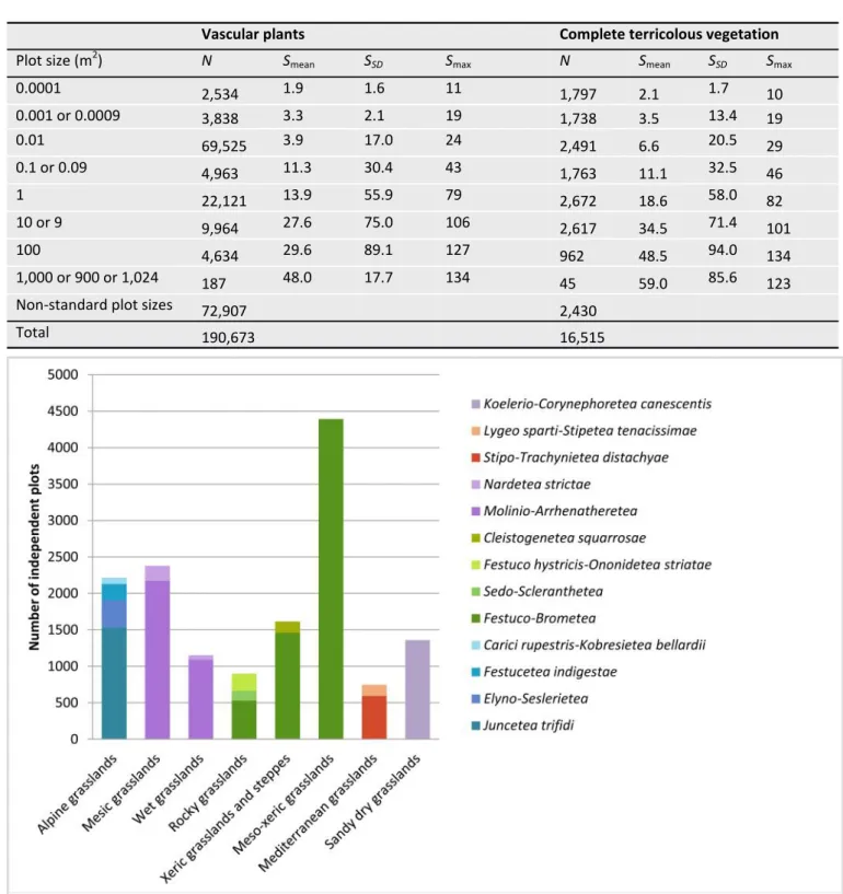
58,977 plots) and Austria the highest density (16.58 plots per 100 km²) of the total plots. Switzerland has the highest number (5,172 plots) and Andorra the highest density (16.45 plots per 100 km2) of independent plots (Table 5). Data locations range from sea level to 5,750 m a.s.l., with the largest frac-tion of independent plots coming from 101–1,000 m a.s.l. (Table 4). Sampling year is one of the metadata included for each plot, and this shows that data were sampled between 1948 and 2018, with 59.3% of all independent plots sur-veyed between 2010–2019 (Table 4). Currently, 98% of all independent plots have been assigned to one of 22 vegeta-tion types (Table 6), with 79% of plots being syntaxonomi-cally assigned to a class and/or subordinate syntaxa. Natural grasslands, secondary grasslands and azonal habitats are the most frequent broad groups. Within these groups, al-pine grasslands and xeric grasslands and steppes, meso-xeric and mesic grasslands and saline communities and wet-lands, respectively, are the most frequent vegetation types (Table 6). With respect to azonal communities, Juncetea maritimi and Scheuchzerio palustris-Caricetea fuscae are the most frequent phytosociological classes in saline communi-ties and wetlands, respectively. The distribution of phytoso-ciological classes across the natural and secondary grassland types is shown in Fig. 4. The temperate dry grassland class Festuco-Brometea (23%) is present in rocky grasslands, meso-xeric grasslands and xeric grasslands and steppes, but most plots correspond to meso-xeric grasslands. The class Molinio-Arrhenatheretea (12%) is well represented in mesic and wet grasslands, while the best-represented classes in alpine and sandy dry grasslands are Juncetea trifidi and Koelerio-Corynephoretea canescentis, respectively (Fig. 4). The most frequent standard-plot sizes are 0.01 m², followed by 1 m² and 9–10 m² (Table 7). Data of the complete vegeta-tion (vascular plants, and terricolous bryophytes and li-chens) are available for 16,515 plots (8.7%) (Table 7). Meth-odologically, the majority of contributors used shoot sam-pling rather than rooted samsam-pling (Table 4), which can make a big difference for the assessment of vascular plant rich-ness at small spatial grains (Dengler 2008; Güler et al. 2016; Cancellieri et al. 2017). Among plot shapes, squares wereFig. 2. Spatial distribution of the independent plots contained in GrassPlot v. 2.00 shown as plot density in equally-sized grid cells of 10,000 km2 (N = 28,171).
Fig. 3. Spatial distribution of the nested-plot series with at least four grain sizes contained in GrassPlot v. 2.00 shown as plot density in equally-sized grid cells of 10,000 km2 (N = 4,654).
most frequently employed (82%), followed by circles (18%) but rectangles are rarer. GrassPlot’s geographic coordinates most often have an accuracy of < 1 km and in 18%, of < 1 m (Table 4).
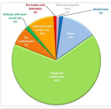
As explained above, header data in GrassPlot also hold many structural (e.g. cover and height of vegetation layers, biomass) and ecological (e.g. topography, soil, land use) parameters that have harmonized terminology and units of measurement. The distribution of plots across biomes and regions is shown in Fig. 5 and Table 8, respectively.
Governance, applications and outlook
GrassPlot is a self-governed consortium, associated with the Eurasian Dry Grassland Group (EDGG). The data contribu-tors remain owners of their data and become members of the consortium. Every two years, the consortium elects from its members a seven-strong Governing Board. Since 27 February 2019, the Governing Board is composed of Jürgen Dengler (Switzerland; custodian), Idoia Biurrun (Spain, dep-uty custodian and database manager), Sabina Burrascano (Italy), Iwona Dembicz (Poland and Switzerland), Riccardo Guarino (Italy), Jutta Kapfer (Norway) and Remigiusz Pielech (Poland). Other consortium members act as additional data managers, such as Itziar García-Mijangos, Salza Palpurina, Anne Mimet, Corrado Marcenò and Vincent Pellissier. Rights and duties of data contributors and data users are regulated
in Bylaws, of which a slightly modified version was adopted by the GrassPlot Consortium on 1 January 2019. The Grass-Plot website is currently hosted at the Ecoinformatics Portal Bayreuth (https://bit.ly/2HvVkgu), but will be transferred shortly to the new EDGG website (http://www.edgg.org). As already mentioned, the purpose of GrassPlot is to pro-vide high-quality data for broad-scale analyses of various aspects of vegetation diversity. According to the GrassPlot Bylaws, members of the consortium can request data for research projects (and non-members can join up with a member to do so). Currently, one such paper project has been completed and three are under way. Dengler et al. (2019) recently analysed which function best describes spe-cies-area relationships (SARs) in Palaearctic grasslands. In a follow-up paper (J. Dengler, I. Dembicz et al., in prep.), the authors will test how the exponent of the power function (z-value) as a measure of small-scale beta-diversity depends on taxonomic group, vegetation type and site conditions. Furthermore, an overview of mean, minimum and maxi-mum richness data of Palaearctic grasslands across regions, vegetation types, taxa and scales will serve as a major benchmarking tool both for fundamental research and con-servation and is well-developed (I. Biurrun et al. in prep.). In addition, an online reference database is planned for publi-cation along with this study. Finally, the relationship be-tween sampling grain and beta-diversity is now being tested
Table 5. Number (N) and density of plots per country (or dependent territory), sorted by decreasing density of independ-ent plots (N = 28,171). The twindepend-enty five countries with the highest densities are listed. Area [km²] refers to the size of the respective territory. For comparison columns Nall and Nall / 100 km2 provide numbers and densities of all plots for the
listed countries (Nall = 190,673).
Code Country Area [km²] N N / 100 km² Nall Nall / 100 km²
AD Andorra 468 77 16.45 77 16.45 CH Switzerland 41,285 5,172 12.52 6,134 14.86 HU Hungary 93,030 2,638 2.84 4,320 4.64 EE Estonia 45,100 832 1.84 1,578 3.50 AT Austria 83,855 1,401 1.67 13,899 16.58 DE Germany 356,840 3,684 1.03 8,359 2.34 ES Spain 504,790 3,451 0.68 58,977 11.68 AZ Azerbaijan 86,600 408 0.47 2,033 2.35
SJ Svalbard and Jan Mayen 61,397 280 0.46 280 0.46
IL Israel 20,724 82 0.39 1,795 8.66 LV Latvia 64,589 250 0.39 250 0.39 CZ Czech Republic 78,864 280 0.36 1,396 1.77 BE Belgium 30,688 90 0.29 90 0.29 BG Bulgaria 110,910 315 0.28 844 0.76 HR Croatia 56,594 160 0.28 227 0.40 NO Norway 323,758 911 0.28 15,292 4.72 SK Slovakia 49,035 139 0.28 477 0.97 IT Italy 301,245 742 0.25 15,120 5.02 UK United Kingdom 244,587 586 0.24 3,756 1.54 SE Sweden 440,940 1,000 0.23 26,219 5.95 PL Poland 312,685 620 0.20 3,148 1.01 RO Romania 238,397 436 0.18 1,354 0.57 SI Slovenia 20,273 37 0.18 37 0.18 UA Ukraine 603,628 765 0.13 2677 0.44 RS Serbia 77,453 119 0.15 533 0.69
Table 6. Distribution of plots in GrassPlot v. 2.00 across the 22 vegetation types and five broad groups. N = number of independent plots in each vegetation type and broad group; % GP = proportion of independent plots of each vegetation type in GrassPlot; % VT = proportion of independent plots of a phytosociological class inside each vegetation type. If the values in % VT do not sum up to 100% within one vegetation type, this is due to plots without assignment to a phytosoci-ological class, and also due to the fact that only classes with more than 10% VT are shown (with some exceptions). [NA] in the column Group indicates the number of plots that have not been assigned to any vegetation type. [NA] in the col-umn Phytosociological class indicates that plots of this vegetation type do not have phytosociological assignment; assig-nation to vegetation type has been made manually.
Group Vegetation type N % GP Phytosociological class % VT
Natural grasslands (N = 6,222) Alpine grasslands 3,023 10.7 Elyno-Seslerietea 12.5 Festucetea indigestae 7.3 Juncetea trifidi 50.5
Alpine steppes 89 0.3 [NA] -
Rocky grasslands 948 3.4
Festuco hystricis-Ononidetea striatae 24.6
Festuco-Brometea 56.6
Sedo-Scleranthetea 14.1
Xeric grasslands and steppes 2,162 7.7 Cleistogenetea squarrosae 7.2
Festuco-Brometea 67.5
Secondary grasslands (N = 11,902)
Wet grasslands 1,375 4.9 Molinio-Arrhenatheretea 79.2
Mesic grasslands 3,627 12.9 Molinio-Arrhenatheretea 59.9
Meso-xeric grasslands 4,542 16.1 Festuco-Brometea 96.7
Mediterranean grasslands 817 2.9 Lygeo sparti-Stipetea tenacissimae 18.7
Stipo-Trachynietea distachyae 72.7
Sandy dry grasslands 1,541 5.5 Koelerio-Corynephoretea canescentis 88.3
Azonal habitats (N = 7,333)
Wetlands 2,700 9.6
Oxycocco-Sphagnetea 10.9
Phragmito-Magnocaricetea 13.2
Scheuchzerio palustris-Caricetea fuscae 70.9
Saline communities 2,931 10.4 Juncetea maritimi 70.5
Dunes 953 3.4 Ammophiletea 43.7
Helichryso-Crucianelletea maritimae 50.1
Rocks and screes 356 1.3
Didymophyso aucheri-Dracocephaletea
aucheri 22.1
Thlaspietea rotundifolii 27.2
Saline steppes and
semi-deserts 393 1.4 Festuco-Puccinellietea 100
Dwarf shrublands (N = 900)
Arctic-alpine heathlands 451 1.6 Loiseleurio procumbentis-Vaccinietea 20.6
Lowland heathlands 116 0.4 Calluno-Ulicetea 31.8
Garrigues and Thorn cushion
communities 333 1.2
Festuco hystricis-Ononidetea striatae 2.4
Onobrychidetea cornutae 2.4
Ononido-Rosmarinetea 3.6
Tall forb and ruderal communities (N = 724)
Tall forb and fringe
communities 271 1.0
Molinio-Arrhenatheretea 35.4
Mulgedio-Aconitetea 28.0
Trifolio-Geranietea sanguinei 26.9
Ruderal communities 453 1.6 Artemisietea vulgaris 18.9
Epilobietea angustifolii 34.4
Deserts and semi-deserts
(N = 559)
Alpine deserts 11 < 0.1 Ajanio-Cleistogenetea songoricae 72.7
Cold deserts and semi-deserts 519 1.8 [NA] -
Warm deserts and semi-deserts 29 0.1 Kleinio-Euphorbietea canariensis 44.8
Table 7. Number of plots (N), mean richness (Smean) with standard deviation (SSD) and maximum richness (Smax) in Grass-Plot v. 2.00 acrossdifferent plot sizes, and for vascular plants and complete terricolous vegetation (vascular plants, bryo-phytes and lichens), respectively. All plots and subplots have been considered, thus a total of 190,673 plots. Non-standard plot sizes include all other plot sizes (which are collected only in case of nested-plot series). Note that due to different sample sizes (see column N), maxima of larger plot sizes can be lower than for maxima of smaller plot sizes or that maxima of complete terricolous vegetation can be lower than maxima of vascular plants only. Information on plot sizes that deviate by a maximum of 10% (e.g. 9 m² vs. 10 m²), is combined in one row because, based on species-area relationships with typical z-values between 0.15 and 0.30, the relative difference in richness would only be about 1.6– 3.2%, i.e. negligible given the overall variability of the data.
Vascular plants Complete terricolous vegetation
Plot size (m2) N Smean SSD Smax N Smean SSD Smax
0.0001 2,534 1.9 1.6 11 1,797 2.1 1.7 10 0.001 or 0.0009 3,838 3.3 2.1 19 1,738 3.5 13.4 19 0.01 69,525 3.9 17.0 24 2,491 6.6 20.5 29 0.1 or 0.09 4,963 11.3 30.4 43 1,763 11.1 32.5 46 1 22,121 13.9 55.9 79 2,672 18.6 58.0 82 10 or 9 9,964 27.6 75.0 106 2,617 34.5 71.4 101 100 4,634 29.6 89.1 127 962 48.5 94.0 134 1,000 or 900 or 1,024 187 48.0 17.7 134 45 59.0 85.6 123
Non-standard plot sizes 72,907 2,430
Total 190,673 16,515
Fig. 4. Frequency of the natural and secondary grassland types and their assignment to phytosociological classes in Grass-Plot v. 2.00. Alpine steppes are not represented as they are not assigned to any phytosociological class in GrassGrass-Plot. Only independent plots have been considered (N = 28,171). Absolute numbers are shown, so that the presence of each class in different vegetation types can be compared.
across different spatial extents and vegetation types based on composition data (S. Burrascano et al. in prep.).
GrassPlot represents work in progress. Therefore, we wel-come new data contributions that meet the specific criteria of GrassPlot (Dengler et al. 2018; GrassPlot website, http:// bit.ly/2NZ6A9d). Of particular value are datasets that (largely) follow the standardised EDGG multi-scale sampling (Dengler et al. 2016b), specifically if they come from under-represented regions or vegetation types (see Figs. 2 and 3, Table 6). However, as GrassPlot does not have external funding, data preparation and harmonisation has to be un-dertaken voluntarily by the Governing Board and other members and thus it might take a while from data provision to actual inclusion. Likewise, we are also working on im-proving the completeness and consistency of the header data (methodological, geographic, abiotic, land use, struc-tural information) of the contained plots and increasing the fraction of plots with readily available compositional data. We have agreed with the European Vegetation Archive (EVA; Chytrý et al. 2016) and the global vegetation database “sPlot” (Bruelheide et al. 2019) to contribute GrassPlot data not yet included in these two databases once the composi-tional data are ready and provided the data owners contrib-ute. This step will fill important data gaps in EVA and sPlot and give our data contributors the opportunity of additional benefit. Last but not least, we hope that the publication of the first macroecological paper from GrassPlot (Dengler et al. 2019) will raise the awareness of the unique qualities of GrassPlot for such studies and spur many more exciting re-search proposals to be submitted to the Governing Board.
Author contributions
I.B. is the database manager of GrassPlot; she and J.D. planned and led this paper. S.B., I.D., R.G., J.K. and R.P. as further members of the GrassPlot Governing Board as well as I.G.M., V.W., S.P., A.M., V.P, C.M. and A.N. contributed substantially to data preparation, analyses and writting. A.B., S.Bo., A.M.C. J.A.G., A.K., J.A.C., B.E., B.J.A., Z.K., M.M., G.S and K.M added helpful comments, and all other authors contributed data to GrassPlot after v. 1.00, checked and approved the manuscript.
Acknowledgements
We thank the BayIntAn program of the Bavarian Research Alliance (https://www.bayfor.org/en/research-funding/ bayintan.php; grant no. UBT_2017_58) and the Bayreuth Centre of Ecology and Environmental Research (BayCEER;
https://www.bayceer.uni-bayreuth.de/) for funding the GrassPlot workshop in Bayreuth. We thank EDGG and the International Association for Vegetation Science (IAVS) for the continuous support of the EDGG Field Workshops dur-ing which large parts of the GrassPlot data were sampled. We are also grateful to the scientific editor Frank Yonghong Li and the linguistic editor Richard Jefferson.
References
Bruelheide, H., Dengler, J., Jiménez-Alfaro, B., Purschke, O., Hennekens, S.M., Chytrý M., Pillar, V.D., Jansen, F., Kattge, J., (…) & Zverev, A. 2019. sPlot – a new tool for global vegetation analyses. Journal of Vegetation Science 30: 161–186.
Cancellieri, L., Mancini, L.D., Sperandii, M.G. & Filibeck, G. 2017. In and out: Effects of shoot- vs. rooted-presence sampling meth-Fig. 5. Distribution of independent plots contained in
GrassPlot v. 2.00 (N = 28,171) across biomes as defined by Bruelheide et al. (2019).
Table 8. Distribution of independent plots in GrassPlot v. 2.00 according to the regionalization used in Grasslands of
the world (Törok & Dengler 2018) and Encyclopedia of the
world’s biomes (Dengler et al. in press).
Grasslands of the world N %
Western and Northern Europe 13,343 47.4
Eastern Europe 6,598 23.4
Mediterranean and Middle East 5,301 18.8
China and Mongolia 1,762 6.3
Russia 522 1.9
Japan 418 1.5
Kazakhstan and Middle Asia 227 0.8
Encyclopedia of the world’s biomes N %
Western Europe 14,042 49.8
Eastern Europe 5,455 19.4
Northern Europe 3,281 11.6
Mediterranean 1,779 6.3
China 1,291 4.6
Middle East and Caucasus 685 2.4
Russia 522 1.9
Mongolia 471 1.7
Japan and Korea 418 1.5
ods on plant diversity measures in mountain grasslands.
Eco-logical Indicators 72: 315–321.
Cayuela, L, Granzow-de la Cerda, I., Albuquerque, F.S. & Golicher, D. 2012. Taxondstand: An R package for species names stan-dardisation in vegetation databases. Methods in Ecology and
Evolution 3: 1078−1083.
Chytrý, M., Hennekens, S.M., Jiménez-Alfaro, B., Knollová, I., Dengler, J., Jansen, F., Landucci, F., Schaminée, J.H.G, Aćić, S., (...) & Yamalov, S. 2016. European Vegetation Archive (EVA): an integrated database of European vegetation plots. Applied
Vegetation Science 19: 173−180.
Collins, S.L., Knapp, A.K., Briggs, J.M., Blair, J.M. & Steinauer, E.M. 1998. Modulation of diversity by grazing and mowing in native tallgrass prairie. Science 280: 745–747.
Dengler, J. 2008. Pitfalls in small-scale species-area sampling and analysis. Folia Geobotanica 43: 269–287.
Dengler, J., Jansen, F., Glöckler, F., Peet, R.K., De Cáceres, M., Chytrý, M., Ewald, J., Oldeland, J., Finckh, M., (…) & Spencer, N. 2011. The Global Index of Vegetation-Plot Databases (GIVD): a new resource for vegetation science. Journal of Vegetation
Science 22: 582–597.
Dengler, J., Todorova, S., Becker, T., Boch, S., Chytrý, M., Diek-mann, M., Dolnik, C., Dupré, C., Giusso del Galdo, G.P., (…) & Vassilev, K. 2012. Database Species-Area Relationships in Palaearctic Grasslands. Biodiversity & Ecology 4: 321–322. Dengler, J., Biurrun, I., Apostolova, I., Baumann, E., Becker, T.,
Berastegi, A., Boch, S., Dembicz, I., Dolnik, C., (…) & Weiser, F. 2016a. Scale-dependent plant diversity in Palaearctic grass-lands: a comparative overview. Bulletin of the Eurasian Dry
Grassland Group 31: 12−26.
Dengler, J., Boch, S., Filibeck, G., Chiarucci, A., Dembicz, I., Guarino, R., Henneberg, B., Janišová, M., Marcenò, C., (…) & Biurrun, I. 2016b. Assessing plant diversity and composition in grasslands across spatial scales: the standardised EDGG sampling method-ology. Bulletin of the Eurasian Grassland Group 32: 13−30. Dengler, J., Wagner, V., Dembicz, I., García-Mijangos, I.,
Naqinez-had, A., Boch, S., Chiarucci, A., Conradi, T., Filibeck, G., (…) & Biurrun, I. 2018. GrassPlot – a database of multi-scale plant diversity in Palaearctic grasslands. Phytocoenologia 48: 331– 347.
Dengler, J., Matthews, T.J., Steinbauer, M.J., Wolfrum, S., Boch, S., Chiarucci, A., Conradi, T., Dembicz, I., Marcenò, C., (…) & Biur-run, I. 2019. Species-area relationships in continuous vegeta-tion: Evidence from Palaearctic grasslands. Journal of
Biogeog-raphy. DOI: 10.1111/jbi.13697.
Dengler, J., Biurrun, I., Boch, S., Dembicz, I. & Török, P. in press. Grasslands of the Palaeartic realm: introduction and synthesis. In: Goldstein, M.I. & DellaSala, D.A. (eds.) Encyclopedia of the
World’s biomes. Elsevier, Oxford, UK.
Ermakov, N. & Krestov, P. 2009. Revision of the higher syntaxa of meadows in the Russian far east. Vegetation of Russia 14. St. Petersburg, Russia.
Ermakov, N., Larionov, A., Polyakova, M., Pestunov, I. & Didukh. Y.P. 2014. Diversity and spatial structure of cryophitic steppes of the Minusinskaya intermountain basin in Southern Siberia (Russia). Tuexenia 34: 431−446.
Güler, B., Jentsch, A., Bartha, S., Bloor, J.M.G., Campetella, G., Canullo, R., Házi, J., Kreyling, J., Pottier, J., (…) & Dengler, J. 2016. How plot shape and dispersion affect plant species rich-ness counts: implications for sampling design and rarefaction analyses. Journal of Vegetation Science 27: 692–703.
Hudson, L.N., Newbold, T., Contu, S., Hill, S.L.L., Lysenko, I., De Palma, A., Phillips, H.R.P., Senior, R.A., Bennett, D.J., (…) &
Pur-vis, A. 2014. The PREDICTS database: A global database of how local terrestrial biodiversity responds to human impacts.
Ecol-ogy and Evolution 4: 4701–4735.
Hüseynova, R. & Yalçin, E. 2018. Subalpine vegetation in Giresun Mountains (Turkey). Acta Botanica Croatica 77: 152−160. Kuzemko, A.A., Steinbauer, M.J., Becker, T., Didukh, Y.P., Dolnik, C.,
Jeschke, M., Naqinezhad, A., Ugurlu, E., Vassilev, K. & Dengler, J. 2016. Patterns and drivers of phytodiversity of steppe grass-lands of Central Podolia (Ukraine). Biodiversity and
Conserva-tion 25: 2233−2250.
Mucina, L., Bültmann, H., Dierßen, K., Theurillat, J.-P., Raus, T., Čarni, A., Šumberová, K., Willner, W., Dengler, J., (…) & Tichý, L. 2016. Vegetation of Europe: Hierarchical floristic classification system of vascular plant, bryophyte, lichen, and algal commu-nities. Applied Vegetation Science 19 (Suppl. 1): 3−264. Niedrist, G., Tasser, E., Lüth, C., Dalla Via, J. & Tappeiner, U. 2009.
Plant diversity declines with recent land use changes in Euro-pean Alps. Plant Ecology 202: 195−210.
Noroozi, J., Willner, W., Pauli, H. & Grabherr, G. 2014. Phytosociol-ogy and ecolPhytosociol-ogy of the high-alpine to subnival scree vegetation of N and NW Iran (Alborz and Azerbaijan Mts.). Applied
Vegeta-tion Science 17: 142−161.
Nowak, A., Nobis, A., Nowak, S. & Nobis, M. 2018. Classification of steppe vegetation in the eastern Pamir Alai and southwestern Tian-Shan Mountains (Tajikistan, Kyrgyzstan). Phytocoenologia 48: 369−391.
Pauli, H., Gottfried, M., Dullinger, S., Abdaladze, O., Akhalkatsi, M., Benito Alonso, J.L., Coldea, G., Dick, J., Erschbamer, B., (…) & Grabherr, G. 2012. Recent plant diversity changes on Europe’s mountain summits. Science 336: 353−355.
Polyakova, M.A., Dembicz, I., Becker, T., Becker, U., Demina, O.N., Ermakov, N., Filibeck, G., Guarino, R., Janišová, M., (…) & Dengler, J. 2016. Scale- and taxon-dependent patterns of plant diversity in steppes of Khakassia, South Siberia (Russia).
Biodi-versity and Conservation 25: 2251−2273.
R Core Team. 2019. R: A language and environment for statistical
computing. R Foundation for Statistical Computing. Vienna, AT.
Reinecke, J., Troeva, E. & Wesche, K. 2017. Extrazonal steppes and other temperate grasslands of northern Siberia − Phytosoci-ological classification and ecPhytosoci-ological characterization.
Phyto-coenologia 47: 167−196.
Schultz, J. 2005. The ecozones of the world. The ecological division
of the geosphere. 2nd ed. Springer, Berlin, DE.
Török, P. & Dengler, J. 2018. Palaearctic grasslands in transition: overarching patterns and future prospects. In: Squires, V.R., Dengler, J., Feng, H. & Hua, L. (eds.) Grasslands of the world:
diversity, management and conservation: pp. 15–26. CRC Press,
Boca Raton, US.
Turtureanu, P.D., Palpurina, S., Becker, T., Dolnik, C., Ruprecht, E., Sutcliffe, L.M.E., Szabó, A. & Dengler, J. 2014. Scale- and taxon-dependent biodiversity patterns of dry grassland vegetation in Transylvania (Romania). Agriculture, Ecosystems &
Environ-ment 182: 15–24.
Wehrden, H. von, Wesche, K. & Miehe, G. 2009. Plant communities of the southern Mongolian Gobi. Phytocoenologia 39: 331−376.
Wickham, H. & Henry, L. 2019. tidyr: Easily Tidy Data with 'spread
()' and 'gather()' Functions. R package version 0.8.3. https:// CRAN.R-project.org/package=tidyr.
Wickham, H., Francois, R., Henry, L. & Müller, K. 2017. dplyr: A
Grammar of Data Manipulation. R package version 0.7.4.
Appendix 1. Example of species composition in a nested-plot series prepared in long format in GrassPlot v. 2.00.
GrassPlot.plotID Area.m2 GrassPlot.ID.largest. nested
Species.original Group Layer Abundance Abundance_ Scale
EU_F_N001_0.0001aa 0.0001 EU_F_N001_100 Eryngium
maritimum
V H 1 P/A
EU_F_N001_0.0001ab 0.0001 EU_F_N001_100 Ammophila
arenaria subsp. australis
V H 1 P/A
EU_F_N001_0.0001ab 0.0001 EU_F_N001_100 Calystegia
soldanella
V H 1 P/A
EU_F_N001_0.0001bb 0.0001 EU_F_N001_100 Calystegia
soldanella
V H 1 P/A
EU_F_N001_0.001aa 0.001 EU_F_N001_100 Eryngium
maritimum
V H 1 P/A
EU_F_N001_0.001ab 0.001 EU_F_N001_100 Ammophila
arenaria subsp. australis
V H 1 P/A
EU_F_N001_0.001ab 0.001 EU_F_N001_100 Calystegia
soldanella
V H 1 P/A
EU_F_N001_0.001bb 0.001 EU_F_N001_100 Calystegia
soldanella
V H 1 P/A
EU_F_N001_0.01aa 0.01 EU_F_N001_100 Eryngium
maritimum
V H 1 P/A
EU_F_N001_0.01ab 0.01 EU_F_N001_100 Ammophila
arenaria subsp. australis
V H 1 P/A
EU_F_N001_0.01ab 0.01 EU_F_N001_100 Calystegia
soldanella
V H 1 P/A
EU_F_N001_0.01ab 0.01 EU_F_N001_100 Euphorbia
paralias
V H 1 P/A
EU_F_N001_0.01ba 0.01 EU_F_N001_100 Galium
arenarium
V H 1 P/A
EU_F_N001_0.01bb 0.01 EU_F_N001_100 Calystegia
soldanella
V H 1 P/A
EU_F_N001_0.1aa 0.1 EU_F_N001_100 Calystegia
soldanella
V H 1 P/A
EU_F_N001_0.1aa 0.1 EU_F_N001_100 Elytrigia juncea
subsp.
boreoatlantica
V H 1 P/A
EU_F_N001_0.1aa 0.1 EU_F_N001_100 Eryngium
maritimum
V H 1 P/A
EU_F_N001_0.1ab 0.1 EU_F_N001_100 Ammophila
arenaria subsp. australis
V H 1 P/A
EU_F_N001_0.1ab 0.1 EU_F_N001_100 Calystegia
soldanella
V H 1 P/A
EU_F_N001_0.1ab 0.1 EU_F_N001_100 Eryngium
maritimum
V H 1 P/A
EU_F_N001_0.1ab 0.1 EU_F_N001_100 Euphorbia
paralias
V H 1 P/A
EU_F_N001_0.1ab 0.1 EU_F_N001_100 Hieracium
eriophorum
V H 1 P/A
EU_F_N001_0.1ba 0.1 EU_F_N001_100 Ammophila
arenaria subsp. australis