An analysis of the gender wage gap in Peru in the formal and informal sectors

(1)

An analysis of the gender wage gap in Peru in the formal and

informal sectors

MSc in Economics, Universitat de Barcelona

Author

Richar Quispe Cuba

Advisor

Raul Ramos Lobo

June 18, 2020

Abstract

Unlike previous studies on gender gaps, this research analyzes wage gaps within the Peruvian labor market considering its segmentation between informal and formal and a sub-segmentation between public and private, generating 4 segments in the labor market. For this purpose, we apply decomposition methods for mean wage and along the wage distribution. The main findings are the following: first, in the informal segment there are wide wage gaps in the upper and lower ends of the distribution against women with a greater emphasis on the informal public segment, and in the informal private segment we found a negative wage gap against women but constant along the distribution. Then, in the formal segment (public and private) the largest gaps were found at the upper end of the distribution, a result that is in line with the "glass ceiling" effect found by the international literature.

Keywords: Gender, wage gap, formal, informal, public, private JEL classification: J16, J31, J45, J46, E26

Acknowledgements: Foremost, I would like to thank my advisor, Professor Raul Ramos for all his support and patience, and also thank my family for having trusted and supported me throughout my career. I thank all the people who supported me in this great challenge, since without their support the result would not have been possible.

(2)

1. Introduction

Despite the remarkable growth of the Peruvian economy in the last 20 years, informality continues to be a structural problem that is shared by developing countries. According to INEI (National Institute of Statistics and Informatics ), 7 out of 10 individuals of working age are informal, a situation that does not guarantee basic aspects such as the social security system, health insurance, access to new markets through exports, access to credit, benefits tributaries, among others. This situation is accompanied by various peculiar characteristics of the Peruvian labor market; (Cling, et al., 2014) indicates that 75% of income comes from wages, and that more than half of urban workers work in companies in the informal sector. These data suggest that there is a high relationship between wages and informality. Furthermore, when in Peru around 99% of formal companies are micro and small enterprises, which employ 58% of the economically active population (PRODUCE, 2018) , it is for this reason that the formalization of small companies is sought, since if achieved, it would generate an improvement in the labor market and high tax revenues. On the other hand, according to data from Peru, in the last year 2.1% and 2.2% of jobs were generated for men and women respectively; these jobs were especially for workers with non-university and university higher education (MTPE, 2020), this implies that there has been an increase in the education of workers, these being more qualified. Despite the high growth of developing economies, Peru being 4.8% in the last 10 years; countries in Latin America continue to have the highest rates of wage inequality (ILO, 2018; Wodon & Briere, 2018), that is, a negative relationship between them still persists. Among all the characteristics of the labor market, we will focus on analyzing wage gaps, more specifically in the formal and informal sectors.

Globally, great progress has been made in gender equality, which is why from the Global Gender Gap Index 2020, we can see that there is no country that has closed its gap completely (WEF, 2019), the first places are occupied by the Nordic countries and Nicaragua. Furthermore, Peru is in position 66 with an index of 0.714. It is also important to mention that Peru obtained 0.65 in the subindex of the area of economic participation and opportunities, which means that women are 35% less likely to have equal economic participation. Furthermore, this gender inequality generates a cost in national wealth (Lange et al., 2018) since human capital is measured as a cost of the future income of the labor force. It is important to mention that in Latin America and the Caribbean women receive an average labor income of 17% lower than men, having the same characteristics; this occurs despite significant long-term changes, since on average women with higher education exceed that of men, that is 40% of working women have higher education compared to 25% of men (ILO, 2019)

Currently in Peru there is a strong persistence of a wage gap between men and women over time, despite the fact that women have increased their level of labor participation by 73.3% and their level of education is now very high, this wage gap it has gone from 32.2% in 2004 to 28.6% in 2018 (MTPE, 2020), that is, on average, men have incomes around S/. 15891_{and the women of S/. 1135. It is also}

important to consider the segmentation of the labor market, since having 72.4% informality, we can clearly see that the labor market is divided into two, on the one hand the informal sector, where labor regulations are non-existent and the characteristics of individuals are similar: low level of education, low income, no contract, among others; and on the other hand the formal sector where labor regulations protect workers against various risks. But in both there is wage discrimination, with a greater emphasis on the informal sector, since people with low educational levels and in a developing

(4)

economy such as Peru, it is common to see that men have a job, and women work at home. So we can distinguish that there is a double punishment in the informal sector for women; one for working informally, since they do not receive work benefits, so they earn very little money and a second punishment for being a woman, since in this sector there is more acceptance for men than for women because of physical abilities are more important than cognitive skills in this sector.

Unlike previous studies that focus on market structure, this research contributes to the little evidence that exists in labor market segmentation, which makes sense from dual labor market research (Doeringer, 1971) . In this study we are going to analyze the gender wage gap in 4 segments: public informal, public formal, private formal and private informal, for which we use various decomposition methods, on average and in along the wage distribution. We use data from the ENAHO (National Household Survey, 2018), which already generates a division of formal and informal individuals, a methodology carried out by the INEI and the ILO (International Labour Organization), the population we use is that of the economically active population, individuals between 14 and 65 years. The results obtained reveal that there is a significant wage gap between male and female workers in all segments, largely due to differences in the endowments of unobservable characteristics; except for the formal public segment where the gap is positive, that is, the wage differences are in favor of women, this is somewhat expected since in this sector the rules are applied as established by law, and since women have greater educational level, generates higher wages for them. Another important finding is that the level of occupation and sector are the variables that generate these salary differences, since as Peru is a very heterogeneous country, each sector and occupation have salaries already defined by the market, so these are variables that determine wages in the labor market. On the other hand, the results of the regression by quantiles show the effect called "glass ceiling" since the wage gap is wider at the top of the distribution and the "sticky floor" effect since the wage gap is wider in the lower part of the wage distribution, both effects for the formal public segment and only the "glass ceiling" effect for the informal public and private informal segments. In addition, for the private formal segment there is a high gap against women but stable (almost linear) along the distribution, this is due to informal practices in the public sector.

The rest of the master's thesis is structured as follows. In the literature section, we examine wage differences in the formal and informal segments, in addition to studies of the gender wage gap both in the mean and along the distribution. In the third section we present the data and the methodologies used, while in the fourth section we present the evidence obtained and end by summarizing the main conclusions.

(5)

2. Literature review

2.1. Theorical

Wage discrimination occurs when two people with the same skills perform similar jobs, but are treated differently by the employer, this difference can have results that translate into different types of remuneration. However, wage gaps cannot only be attributed to discrimination. That is why since seminal work (Gary S. Becker, 1957) he mentioned two important aspects to explain wage differentials between workers: First the theory of human capital where she explains the differences in productivities between men and women; and second, female discrimination in the labor market, which causes inefficiencies. Later, more developed work is done, starting with the decomposition of Oaxaca Blinder (Oaxaca, 1973) that considers the Mincer equation for workers, estimating the differential in wages between men and women, decomposing the wage differential into one part explained and another unexplained, and finds that this differential in average wages is quite large. Subsequently, extensions were made to the Oaxaca-Blinder methodology, since the latter applies decomposition techniques to the mean. Therefore Machado & Mata (2005) use a method based on the estimation of marginal wage distributions consistent with a distribution estimated by regression by quantiles along wage distribution. Then Albrecht et al. (2009) extend the model making corrections for selection bias. Subsequently, estimators of unconditional covariate functions were proposed by Melly (2006) using Monte Carlo simulations that work well on finite samples, and also decompose the wage differential into an explained part (characteristics) and an unexplained part (coefficients). Finally Firpo et al. (2009), proposes to evaluate the changes in the quantiles of the unconditional distribution, for which it uses an influence function regression (RIF), they decompose the wage differential in the mean and along the distribution, also in a part explained and unexplained.

2.2. Empirical evidence

The concept of segment in the labor market was introduced by Peter B. Doeringer (1971.) Since their seminal contributions have related the gender gap to this concept dividing the labor market by formal and informal sector and by public and private sector. For example Cho & Cho (2011) show a substantial drop in size of the wage gaps in Korea, which is reflected by the unobserved capacity of the workers and considers that there is a simultaneity in the structure of the labor market and gender discrimination. Also, Ben Yahmed (2016) mentions that in Brazil the informal wage gap is 13%, while for the formal sector it is 5%, this is because women have better observable characteristics than men, such as education. Furthermore, Giordano et al. (2011) shows that the premium wage is higher for women and less developed countries in public sector workers; for Australia Barón & Cobb-Clark (2010) analyze the wage gap in the public and private sector, find an important effect in occupational segregation where the wage gap in low-wage workers is explained by the differences in the characteristics related to the wages but not fully explained by high-wage workers.

More recent research has also expanded the analysis beyond the mean considering gender gaps along the wage distribution and specific cases. For example, for the United Kingdom, Olsen & Walby (2004) show segregation in certain occupations in women and in small companies, which were responsible for 36% of the gender pay gap. In Greece, Livanos & Pouliakas (2012) calculate the gender wage gap considering education the most important factor, they show that this gap is around 8.4%, since women generally opt for a less risky education, that is why that women obtain lower wage premiums in the

(6)

labor market. Beaudry & Lewis (2014) consider the importance of people's abilities (cognitive, interpersonal and physical), it shows that the wage gap decreased during the 80s, while returns to education increased, that is, this decrease it was because people were able to adapt to technological change. Gauchat et al., (2012) and Oostendorp (2009) find that the gender wage gap tends to decrease with respect to globalization and trade, especially in richer countries. In Latin America these studies are more representative, since there is a much greater wage inequality, for example, in Chile, Montenegro (2001) uses the methodology of Machado & Mata (2005), it is shown that in the lower part of the salary distribution women have higher returns to education, but similar returns to men in experience; Furthermore, it is shown that at the bottom there is a gap of 10% and at the top around 40%. In Uruguay Borraz & Robano (2010) also uses the Machado and Mata methodology using the extension of Albrecht et al. (2009) shows that the gender wage gap increased throughout the distribution, showing the effect called "ceiling glass”, it was also found that if all women worked, the wage gap could be greater.

In Peru there is little research that talks about the gender gap in the labor market. The most relevant research was carried out by Ñopo (2009) where it uses the matching comparison methodology and shows that one in four workers has characteristics that are not comparable to workers of the opposite sex, and that the wage gap is approximately 28%. Pozo (2017) uses the Machado and Mata methodology and finds that there is a decrease in the gap as we advance to the upper parts of the distribution.

In the literature we find that the wage gap can be studied taking into consideration different aspects, for example, by urban area, by occupational segregation, by type of skills, among others. In all cases we find a significant gap that shows that this problem must be studied in depth.

3. Data and methodology

3.1. Data sources

The source from which the microdata is extracted in this study is the ENAHO (National Household Survey), the ENAHO is designed as a cross-sectional database, where we have quarterly and annual information, which is designed by the INEI (National Institute of Statistics and Informatics). The objective of this survey is to know the evolution of poverty and the living conditions of the households with coverage at the national level2_{, in the urban and rural areas and in the 24 departments of Peru.}

ENAHO is the main source of information for the generation of indicators such as the characteristics of housing, individuals, health, education, employment, among others. Something important is that the survey has maintained the same format since 2004, so the indicators can be compared year after year.

This survey is subdivided into sections, one of which is employment (Module 500), which we use, in this module the target population is individuals over 14 years of age, in our case we have only considered individuals between 14 and 65 years of age, the which represents the PEA (Economically Active Population). The most important variable to consider is informality, which is built by INEI, based on the methodology proposed by the ILO, this methodology takes into account the

2_{Members of the armed forces who live in barracks, camps, ships, and others are excluded from the survey. People} residing in collective housing (hotels, hospitals, religious asylums and cloisters, prisons, etc.) are also excluded.

(7)

characteristics of the business or establishment where the individual works, and there is information from the year 2012. It is also made an update in the survey in relation to the sector where the individual works, which is based on the International Standard Industrial Classification of all economic activities (ISIC rev. 4); In addition, for the occupation of the individual, the International Standard Classification of Occupations (ISCO-2015) is considered, both cases are used to make them internationally comparable.

In addition, the data source provides information on the characteristics of the people: age, sex, experience, marital status and education; related to employment: occupation, type of contract and if the job is part-time full-time; related to geography: urban or rural, division of macro regions, and finally related to the company: sector where it operates, company size and whether the company is formal or informal. Wage information is used as a transformed variable to obtain hourly wages for the main occupation, which is calculated by dividing the monthly salary by the number of hours worked in a month. It´s important mention that wages are imputed3_{and deflated}4_{, it also includes overtime,}

bonuses, mobility, commissions, among other types of income. For the construction of the data, people older than 65 years were excluded and only individuals who have reported any income were considered. The final sample of the information was 26,806 observations, which correspond to 15768 men and 11038 women, also 15202 observations in the informal sector and 11064 observations in the formal sector, in addition to 19689 observations in the private sector and 6025 in the public sector. Descriptive statistics for the sample can be found in Table A.1 in the Appendix.

3.2. Methods

This research applies three different decomposition techniques to analyse the differential in wages between men and women. The first is the Oaxaca-Blinder methods (Blinder, 1973; Oaxaca, 1973), which allows detailing the decomposition into observable explanatory variables and unobservable characteristics between men and women in the mean. The second and third methodology are based on determining the wage differential along the distribution, in the first case we have applied Melly (2006) who uses unconditional covariate functions using Monte Carlo simulations and for the second case we have applied Firpo et al. (2009) that use a recentered influence function.

3.2.1. Oaxaca – Blinder (1973)

The Oaxaca-Blinder methodology is based on separating the estimation in two, one in the difference existing from a common component (explained), and the other due to other factors (unexplained). We assume the mincerian equation. The expression can be expressed as follows:

𝑤𝑖 = 𝑋𝑖𝛽 + 𝜀𝑖 (1)

3 The imputation process is carried out in two stages: a) First stage corresponds to the allocation of qualitative characteristics to household members who did not report the education (chap. 300), health (chap. 400) and employment (chap. 500) modules, leaving the quantitative variables as missing values. The Hot Deck technique is used to impute the qualitative variables. b) Second stage, values are assigned to the quantitative variables that were recorded as missing values (information not declared by the informant). For the imputation of the quantitative variables, the Median Matrices technique is used, thus guaranteeing that the assigned value is not influenced by extreme values.

4 Deflated is the process of transforming from nominal monetary values to real monetary values (at constant prices for a certain period), through the application of a price index that eliminates the effect of prices in the analysis period.

(8)

Where 𝑤𝑖 represents the logarithm of the hourly wage of worker i and 𝑋𝑖 represents the different

individual characteristics, characteristics of employment and companies. First we separate the equation between men and women where E (w) is the expected value of the variable, to later take differences:

𝐷 = 𝐸(𝑊𝑀) − 𝐸(𝑊𝐹) = 𝐸(𝑋𝑀𝛽 + 𝜀𝑀) − 𝐸(𝑋𝐹𝛽 + 𝜀𝐹) (2)

By property of the expected value we have the following:

𝐸(𝑋𝑖𝛽) = 𝐸(𝑋𝑖)𝛽 and 𝐸(𝜀𝑖) = 0 (3)

Therefore, we have the following:

𝐷 = 𝐸(𝑊𝑀) − 𝐸(𝑊𝐹) = 𝐸(𝑋𝑀)𝛽 − 𝐸(𝑋𝐹)𝛽 (4)

Instead of the expected values we will consider the average values:

𝐷 = 𝐸(𝑊𝑀) − 𝐸(𝑊𝐹) = (𝑊̅𝑀) − (𝑊̅𝐹) (5)

𝑊̅_𝑀 = 𝑋̅_𝑀𝛽_𝑀 ; 𝑊̅_𝐹 _{= 𝑋̅}_𝐹_𝛽_𝐹 (6)

Replacing, we have the following:

𝐷 = 𝑊̅𝑀 − 𝑊̅𝐹 = 𝑋̅𝑀𝛽𝑀 − 𝑋̅𝐹𝛽𝐹 (7)

Adding and subtracting 𝑋̅𝐹𝛽𝑀 :

𝐷 = 𝑊̅_𝑀 − 𝑊̅_𝐹 = (𝑋̅_𝑀 − 𝑋̅_𝐹)𝛽_𝑀 + 𝑋̅_𝐹(𝛽_𝑀 − 𝛽_𝐹) (8) In general, equation (1) is estimated using robust ordinary least squares for both the joint sample of men and women separately, and then decomposing it into the difference in average hourly wages, as in equation (8). Where the 𝑊̅_𝑀_{and 𝑊}̅_𝐹_{are the average hourly wages of men and women. With this} we obtain the decomposition, which is divided into two parts, the first 𝑋̅𝑀 and 𝑋̅𝐹 (left part) as the

part explained by the differences between the observed variables and the second 𝛽𝑀 and 𝛽𝐹 (right

part) the unexplained part which corresponds to the effect of the coefficients.

Both components can be decomposed, this in order to distinguish their contribution to each explained variable. This decomposition presents a problem, since when applying this procedure, the choice of a certain category for the dummy variables can affect the decomposition results, as shown in Oaxaca & Ransom (1994). For this reason, it is solved by applying the normalization of the dummy variables suggested by Yun (2005), this solves the problem and makes an adequate estimate of the real contribution of each variable to the differential.

(9)

3.2.2. Melly (2006)

The proposal made by Melly (2006) to analyze gender wage gap is based on a regression by quantiles, which was initially proposed by Koenker & Bassett (1978), which makes a more flexible analysis than estimation of OLS. Regression by quantiles estimates the effect of the explanatory variables in each percentile of the conditional distribution, this idea was developed by Machado & Mata (2005). Later Melly proposes a procedure to decompose the differences of the quantiles into an unconditional distribution. Melly's estimator uses Monte Carlo simulations, this estimator will be identical to the Machado and Mata estimator if the number of simulations goes to infinity, an advantage of Melly is its consistency is asymptotically normal. The procedure is the next:

First, we estimate a conditional distribution with a regression by quantiles:

𝑄𝜃(𝑊/𝑋) = 𝑋𝑖𝛽(𝜑) (9)

where 𝜑𝜖(0,1) represents the number of quantiles.

Quantile regression is based on minimizing the sum of the absolute values of the deviations between the value of the salary and its predicted value. The quantile regression model assumes that the conditional quantile of wi is linear in X. The vector of coefficients for 𝛽(𝜑) is estimated as follows:

min 𝛽(𝜃){ ∑ 𝜑|𝑤𝑖 − 𝑤_𝑖≥𝑋_𝑖𝛽(𝜑) 𝑋_𝑖𝛽| + ∑ (1 − 𝜑)| 𝑤_𝑖≤𝑋_𝑖𝛽(𝜑) 𝑤_𝑖 − 𝑋_𝑖𝛽| } (10)

Second, the conditional distribution is integrated over the ranges of the covariates. Integrating on all quantiles and on all observations, 𝛽̂(𝛽̂(𝜑1), . . . , (𝛽̂(𝜑𝑗), . . . , (𝛽̂(𝜑𝐽)), where j=1,…,J. Furthermore,

the unconditional estimator 𝜃 of the dependent variable is given by:

𝑞(𝜃, 𝑋, 𝛽) = 𝑖𝑛𝑓{𝑞:1 𝑛∑ ∑(𝜑𝑗 − 𝜑𝑗−1)(𝑋𝑖𝛽̂(𝜑𝑗) ≤ 𝑞) ≥ 𝜃 𝐽 𝑗=1 𝑁 𝑖=1 } (11)

Now we can estimate the counterfactual distribution and separate the difference of each quantile from the unconditional distribution in: part unexplained by the coefficients and part explained by characteristics:

𝑞(𝜃, 𝑋_𝑀, 𝛽_𝑀) − 𝑞(𝜃, 𝑋_𝐹, 𝛽_𝐹) = [𝑞(𝜃, 𝑋_𝑀, 𝛽_𝑀) − 𝑞(𝜃, 𝑋_𝑀, 𝛽_𝐹)] + [𝑞(𝜃, 𝑋_𝑀, 𝛽_𝐹) − 𝑞(𝜃, 𝑋_𝐹, 𝛽_𝐹)] (12)

Where the first bracket represents the effects of differences in coefficients (discrimination) and the second bracket represents the effects of differences in the distribution of the characteristics. In this case, as in the Oaxaca-Blinder methodology, the variables used for the estimation are the same, that is, characteristics of workers, characteristics of employment and companies.

(10)

3.2.3. Firpo, Fortin, and Lemieux (2009)

This methodology proposes an improvement to the development of the decompositions of the differences between the distributions of a variable. Which is to do an unconditional quantile regression using recentered influence function (RIF). The technique is developed in three steps, the first is to make a substitution of the dependent variable for a transformation, which is the recent influence function (RIF), second, we have to divide the salary distribution into a composition and structure effect using a weighted procedure (the weights are estimated), third, is to make the estimation using the Oaxaca Blinder procedure.

The influence function measures the effect on distribution statistics of small changes in the underlying distribution. Fortin (2011) proposes that the recent influence function should be 𝑅𝐼𝐹(𝑊; 𝜑𝜃) =

𝜑_𝜃+ 𝐼𝐹(𝑊; 𝜑_𝜃), they define unconditional quantile regression as the conditional expectation of

𝑅𝐼𝐹(𝑊; 𝜑𝜃) dado 𝑋: 𝐸[𝑅𝐼𝐹(𝑊; 𝜑𝜃)|𝑋].

The influence function (IF) for a quantile 𝜃𝑡 is equal to:

𝐼𝐹(𝑊; 𝜑_𝜃) = 𝜃 − 𝑙{𝑊 ≤ 𝜑_𝜃})/𝑓_𝑦(𝜑_𝜃) (13)

Where 𝑓𝑦 is the marginal density function of W. Since the recent influence function is 𝑅𝐼𝐹(𝑊; 𝜑𝜃) =

𝜃_𝑡+ 𝐼𝐹(𝑊; 𝜑_𝜃), we can say the following:

𝑅𝐼𝐹(𝑊; 𝜑𝜃) = 𝜑𝜃+ 𝜃 − 𝑙{𝑊 ≤ 𝜑𝜃})/𝑓𝑦(𝜑𝜃) (14)

The estimated coefficients can be calculated using the Oaxaca Blinder decomposition methodology. Firpo et al. (2007) show that a Blinder-Oaxaca type decomposition based on RIF-regression estimates can be approximated for any distributional statistic, including quantiles. The decomposition is as follows:

D(θ) = X̅_Mβ_M − X̅_Fβ_F (15)

D(θ) = (X̅_M − X̅_F)β ∗ (θ) + { X̅_M(β_M(θ) − β ∗ (θ)) + X̅_F(β ∗ (θ) − β_F(θ))} (16) Where 𝛽𝑀(𝜃) and 𝛽𝐹(𝜃) are the unconditional quantile regression coefficients in men, women and in

the group pool. The 𝑋̅𝑀 and 𝑋̅𝐹 are the average observed characteristics for men and women. The first

component on the right side is caused by differences in characteristics, referring to the explained component, the second component refers to the effects of the coefficients, that is, the unexplained component. Interpretation of the results should be taken with care, especially with the unexplained component as it is subject to misinterpretation and different points of view.

3.3. Application

In this section we are going to explain the models that we are going to use in all the methodologies. Explanatory variables in empirical analysis include geographic characteristics, characteristics of individuals, as well as characteristics of work and establishment. The former serve as controls at the geographic level: zone (urban or rural) and macroregion (North West, Center, South West, South East, North East and Lima), controls for individuals: schooling (measured in years), marital status (single or

(11)

married), controls for work, such as the type of contract (indefinite, partial and without contract), time of employment (full time or part time), occupation (10 categories according to ISIC rev. 4), sector (6 categories according to ISCO-2015). Finally, the characteristics of the establishment, specifically for the type of company (small, medium, and large).

As previously mentioned, due to the heterogeneity of the Peruvian labor market, we have divided it into four segments: Public informal, private informal, public formal and private formal, each of these markets has different characteristics, which makes it necessary to carry out the analysis in a differentiated way.

Informal public

In this first case we have 964 observations, it is the smallest segment in the labor market, where individuals work only in 3 sectors: mining, manufacturing and services; they also work in all occupations except the armed forces. It would be expected that in this sector the activities will be carried out as established by law, since we are in the public sector, but we find ourselves in formal employment that uses informal practices. We also see that the most performed occupations are administrative support, sales and elementary occupations. In this model we do not control for company size, since all observations are related to large companies.

𝐿𝑛 𝑊𝑎𝑔𝑒𝑖 = 𝛽0+ 𝛽1𝑤𝑜𝑚𝑒𝑛 + 𝛽2𝑠𝑐ℎ𝑜𝑜𝑙𝑖𝑛𝑔 + 𝛽3𝑒𝑥𝑝𝑒𝑟𝑖𝑒𝑛𝑐𝑒 + 𝛽4𝑒𝑥𝑝𝑒𝑟𝑖𝑒𝑛𝑐𝑒^2

+ 𝛽5𝑚𝑎𝑟𝑟𝑖𝑒𝑑 + 𝛽6𝑢𝑟𝑏𝑎𝑛 + 𝛽7𝑚𝑎𝑐𝑟𝑜𝑟𝑒𝑔𝑖𝑜𝑛 + 𝛽8𝑐𝑜𝑛𝑡𝑟𝑎𝑐𝑡

+ 𝛽9𝑝𝑎𝑟𝑡𝑡𝑖𝑚𝑒 + 𝛽10𝑠𝑒𝑐𝑡𝑜𝑟 + 𝛽11𝑜𝑐𝑢𝑝𝑎𝑡𝑖𝑜𝑛 + 𝜀𝑖

(17)

Informal private

In this case we have 12898 observations, and it is the largest segment in the labor market, since approximately 72% of informality is found in this segment, especially in small companies, which is a very common feature in developing countries. This segment is occupied by all sectors and all occupations except for the armed forces. This is the invisible activity of the State since it is the segment where taxes are not paid, for example: undeclared domestic work, ambulatory sales, among others. According to Perry et al. (2010), there are two causes for informality, one is via expulsion, that is, you cannot or do not want to incur greater expenses than being formal (bureaucracy for the formalization of a company), and the another is via exclusion, that is, the services provided do not compensate the payments made (lack of access to markets, financing, among others).

𝐿𝑛 𝑊𝑎𝑔𝑒𝑖 = 𝛽0+ 𝛽1𝑤𝑜𝑚𝑒𝑛 + 𝛽2𝑠𝑐ℎ𝑜𝑜𝑙𝑖𝑛𝑔 + 𝛽3𝑒𝑥𝑝𝑒𝑟𝑖𝑒𝑛𝑐𝑒 + 𝛽4𝑒𝑥𝑝𝑒𝑟𝑖𝑒𝑛𝑐𝑒^2 + 𝛽5𝑚𝑎𝑟𝑟𝑖𝑒𝑑 + 𝛽6𝑢𝑟𝑏𝑎𝑛 + 𝛽7𝑚𝑎𝑐𝑟𝑜𝑟𝑒𝑔𝑖𝑜𝑛 + 𝛽8𝑐𝑜𝑛𝑡𝑟𝑎𝑐𝑡 + 𝛽9𝑝𝑎𝑟𝑡𝑡𝑖𝑚𝑒 + 𝛽10𝑠𝑒𝑐𝑡𝑜𝑟 + 𝛽11𝑜𝑐𝑢𝑝𝑎𝑡𝑖𝑜𝑛 + 𝛽12𝑆𝑖𝑧𝑒 𝑜𝑓 𝑐𝑜𝑚𝑝𝑎𝑛𝑦 + 𝜀𝑖 (18) Formal Public

In this case we have 4470 observations and it is the second smallest segment in the Peruvian labor market, it is the segment that is within the parameters regulated by the State, therefore it complies with all current regulations: tax, taxes, environment, labor, among others. This segment is occupied by all occupations, the most common jobs are: public officials (for example in ministries), teachers in public

(12)

schools, doctors in public hospitals, among others. Workers in this sector have medical insurance, in addition to the payment of pensions for social security. In this case we do not control by company size since it is assumed that the entire public system is considered as a large company. The specification is identical to the one shown in equation (17)

Formal Private

In this case we have 6412 observations and the second largest segment of the Peruvian labor market. In general, there are very few small companies in this segment, as it is led by the large companies in Peru. For this reason it is found in all sectors and occupations except for the armed forces. Lima concentrates 50% of private formal employment in the country, and workers have access to social security, a contract, health insurance. All types of companies are concentrated in this segment, which is why we use all variables. All the data can be visualized in the appendix of table A.2. The specification is identical to the one shown in equation (18)

4. Results

4.1. Descriptive evidence

In this section we present statistical information on the main variables for men and women in the Peruvian labor market. The dependent variable is measured as the logarithm of the hourly wage, for men it is 2.0 on average and for women 1.8. In addition, the level of education for men is on average 12.5 years of study and for women it is 12.9 years, this implies that women are more educated than men, but receive lower wages, this may be due to discrimination. Another important fact is the years of experience that for men is an average of 18.5 years and for women it is 17.8 years. In the table it can be seen that the dominant sector is the informal sector, and it is located in the urban area, specifically in Lima, this shows that the labor market is centralized in its capital. We also see that the most relevant sector is services, in occupation, men have greater predominance in elementary occupations (Cleaners, drivers, kitchen helpers and others) and in the case of women there is greater predominance also in elementary occupations and also in the works of services and sales. It is important to mention that the majority of jobs are in small companies, which employ approximately 60% of the PEA (PRODUCE, 2018). We can see this information in the Table A.1.

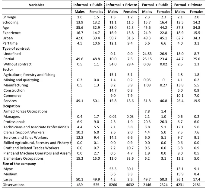
Table A.2 presents the information disaggregated in the 4 segments to be analyzed, where it can be seen that the logarithm of the hourly wage occurs in the public formal sector, being 2.3 for men and women, and the lowest value is for the private informal sector, this being 1.3 for men and 1.2 for women; these two sectors are basically the opposite, since in one the formality guidelines are met at 100%, but in the other case informality is also shown at 100%; as mentioned before, informality represents around 72% of the labor market, which is why it is very important to analyze them separately. The other variables show the information in proportions in the 4 segments for both men and women.

In Figure 1 we show the kernel distributions in the division of the labor market structure (informal and formal) and (public and private) in the logarithm of hourly wages, we see in the graphs that there is no similar behavior that of the average shown in figure 2, this gives us an indication that the labor market should be analyzed separately, since they have independent behaviors. In the graph on the left (informal and formal) we see that the formal sector is skewed to the right, this means that there are higher wages in this sector, also the range of the lower limit is -1.23, which is less than that of the

(13)

average in figure 2, this means that there are fewer people with low wages in this sector, quite the opposite occurs in the informal sector, where the lower limit range is -4.2, this means that most of the informal earn little money. In the graph on the right (public and private), we see that the public sector is more skewed to the right, since they on average have higher wages than those of the private sector, since most companies in the private sector are small companies and in the public sector are large companies. Regarding ranges, we see that in the public sector the lower limit is close to -2.0 and the upper limit is 4.0, which implies that many individuals have high wages, otherwise it happens in the private sector, where the range is much broader, because people are more distributed, in this case we see that there is an accumulation in the lower limit that indicates that individuals have very low wages.

Figure 1

Now in the In figure 2 we show the kernel density of the logarithm of hourly wages between men and women, we can see that they are very similar and slightly asymmetric to the right, with a mean for both cases close to 2.0 logarithmic points and the range fluctuates between -4.2 to 6, and we see that there is an accumulation on the left side of the distribution, this reflects there are many individuals with very low wages. We can also notice that on the average there are slightly more men than women and that they earn more, but we can also notice that in some parts of the distribution the opposite is the case.

(14)

4.2. Decomposition analysis results.

4.2.1 Decomposition analysis in the mean

Oaxaca – Blinder (1973)

Before starting to explain the results of the decompositions of each segment, we have made an estimate using OLS of all the joint data. The information related to the control variables is: education, married, experience, urban and macro regions. As can be seen in Table 1, the gender gap is much smaller in the restricted model, that is, in the model where only women are considered as explanatory (Column 1), but as we add more controls this gap is getting bigger, it varies from 12.8% to 17.7% in favor of men. In column 3, which is the most complete, we control it by informality, the negative sign reflects that the more informality, lower will be the hourly wage and the greater the gender wage gap against women, as in the private sector, since as I explained before this segment concentrates 72% of the labor market. It is important to mention that as the number of observations decreases, the gap increases, that is, this reduction affects women.

Table 1

In table 2 we show the results of the Oaxaca-Blinder decomposition of the 4 segments of the wage gap into the mean value of the wage distributions of men and women, without considering the sample selection bias. The information includes the average size of the wage differential and the values of the two components: characteristics (explained) and coefficients (unexplained). For the first case (informal + public), we show that the wage gap is around 28%, this being the largest of the 4 segments, that is, women in this segment have wages 28% less than men, the unexplained part it represents 76% (0.217) of the gap due to discrimination, and 24% (0.0692) is due to the explained part. In the second case (informal + private), it is the second segment with the largest wage gap and is the largest segment of the labor market since most are micro-companies, the unexplained part represents 101.6% (-2.10) and the part explained represents -1.56% (0.00324), despite the fact that the gap is less than the previous segment, the discrimination is very high due to the work carried out in this segment focusing more on

Variables (1) (2) (3) Women -0.128*** -0.176*** -0.177*** (0.00968) (0.00804) (0.00774) Informal -0.500*** (0.0213) Private -0.231*** (0.0115) Informal*Private 0.0546** (0.0224) Constant 1.941*** 0.220*** 1.284*** (0.00603) (0.02821) (0.0341)

Control variables NO YES YES

Observations 26806 26172 25116

Men 15768 15436 15390

Women 11038 10736 9726

R-squared 0.007 0.358 0.442

Robust standard errors in parentheses *** p<0.01, ** p<0.05, * p<0.1 Elaborated by the author

Control variables are schooling, experience, experience^2, married, urban and Macro regions

(15)

physical than cognitive abilities, that is, more for men than women. In the third case (Formal + public), it is the only segment where the wage gap is positive, that is, women have more wages than men and this is due to the high educational level of women, since occupations in this sector they are more for cognitive abilities than for physical abilities, the unexplained part represents -155%. (-0.0438) and the explained part 255% (0.0720), This is an expected result since in this segment the standards stipulated by "Ministerial Resolution N° 145-2019-TR" are met, through a methodological guide5_{developed by}

the MTPE (Ministry of Labor and Employment Promotion). In the fourth case (Formal + private), we show that the wage gap is 17.9%, this segment is the most complete in the labor market since there are all types of companies, although these are few, the unexplained part represents 115.4% (-2.06) and the explained part -15.4% (0.0275), we clearly see that it is the segment with the highest discrimination in the labor market. We conclude in this part that the private sector is the one with the most discrimination and only the formal public sector has a wage gap in favor of women.

Table 2

In figure 3 and in the appendix in table A.3 we see the detail of those mentioned in the previous table. In general, we see that the occupation and sector variables are that have the highest representativeness in wage gaps and especially in the unexplained part. For example, in the informal private segment, the most relevant variable is occupation in the unexplained part that has a value of -0.361 (see appendix table A.3), since in this sector physical abilities predominate over cognitive abilities, therefore, men have an easier getting a job with a good salary compared to women. In the case of the formal public segment where the gaps are positive, there are two relevant variables that make it positive: one is education (0.0467) in the explained part and the other is the sector (1,306) in the unexplained part, despite the fact that the coefficient is higher, the explaining part has a greater weight, therefore greater importance, which is why education in this sector is the variable that causes the gap to be positive in favor of women. The detail of the other interpretations can be seen in figure 3, where the longest bars

5 This guide is called " Methodological Guide for the Objective Valuation, without Gender Discrimination, of Jobs and Preparation of Tables of Categories and Functions "

Variables Informal + Public Informal + Private Formal + Public Formal + Private Women 1.655*** 1.369*** 2.597*** 2.105*** (0.0291) (0.00985) (0.0105) (0.0129) Men 1.941*** 1.575*** 2.569*** 2.284*** (0.0308) (0.00711) (0.0123) (0.0101) Difference -0.286*** -0.206*** 0.0282* -0.179*** (0.0424) (0.0121) (0.0162) (0.0164) Explained -0.0692** 0.00324 0.0720*** 0.0275 (0.0280) (0.0215) (0.0134) (0.0201) Unexplained -0.217*** -0.210*** -0.0438*** -0.206*** (0.0422) (0.0235) (0.0151) (0.0217) Observations 964 12,898 4,470 6,412

Standard errors in parentheses *** p<0.01, ** p<0.05, * p<0.1 Elaborated by the author

(16)

are analyzed and also in the appendix of table A.3 where the value of the coefficients must be analyzed, but first you have to know which of the variables have greater weight in the salary difference.

Figure 3

4.2.2. Decomposition analysis along the distribution

Melly (2006)

In table 3 we have the results obtained by performing the decomposition of men and women through a quantile regression which allows us to observe the variation in the distribution behind the analysis of means. The wage gap in this case is the difference between the logarithm of the hourly wage for men in a specific quantile of their distribution and the logarithm of the hourly wage for women in the same quantile of their distribution.

According to the table, the null hypothesis is clearly rejected for most quantiles and also throughout the quantile regression process. Therefore, we have estimated 100 separate quantile regressions in each sector through a boopstrap. Then, we have decomposed the differences between the quantiles of the unconditional distributions into a part explained by different characteristic distributions and an unexplained part by different coefficients (could be interpreted as discrimination).

As we can see in Table 3, we have that for the informal public, informal private and formal public the wage differential is negative and significant in all quantiles, that is, women earn less than men in all

(17)

scenarios, which is comparable with the results obtained in Oaxaca Blinder, which is reflected in our table, as the mean. But in the case of formal public, we have a positive sign up to the 60th percentile, then the negative sign appears, this tells us that at the top of the distribution, that is, individuals with very high wages, women earn less than men This indicates that normally high-ranking positions in the public sector such as: Directors, Heads of public institutions, among others, are mostly held by men.

Table 3

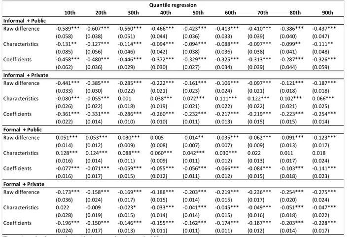
In figure 4 we have the detail of the explained, unexplained part and the total difference in each quantile (we can also see it in the annex to Table A.4). In addition, we mention that the graphs plot the decomposition results with a 95% confidence interval for all estimates. In the first case, informal public we see that the median (50th percentile) is very similar to the value obtained in the Oaxaca methodology, we also see an inverted “U” shape that indicates that in the lower and upper percentile the wage gaps they are larger, especially in the 10th (36%) and 90th (37%) percentiles, with this we demonstrate the effect called “glass ceiling” and “stick floor”, also according to the graph we see that the line of the coefficients is very similar to that of the differences, this indicates that there is a great effect because of unobservable characteristics (discrimination). In the second case, informal private, we also see that the median is similar to the value obtained by Oaxaca, in addition that there is not much fluctuation in the wage difference, this means that the gap is very similar in all the percentiles of the distribution which it varies between 19.5% and 21.6%, in addition to that the line of the effects of the coefficients is very similar to the total differential due to discrimination. This means that in this sector, which is the largest in the labor market, the gap is constant regardless of whether wages are high or low, this is because wages in this sector are close to the minimum wage, in addition there are more predominance of physical than cognitive abilities. In the third case, formal public, we also see that the median is similar to the value obtained in Oaxaca Blinder, the line related to the total differential is lower in the bottom and greater in the upper percentiles, this shows the effect called “ceiling of glass ”, that is, when wages are low there is no discrimination, women earn 10% more than men, but while the percentiles increase, as in the 90th percentile, discrimination increases against women which can be seen in the line of the coefficients, so that women earn 6.9% less than men. In the fourth case, formal private, the median is exactly the same as that of Oaxaca Blinder, we also see that in this segment the effect called “glass ceiling” also occurs, since the greatest gaps are found in the highest percentiles, in this case we see that it is also due to the discrimination that exists in this sector, since the gap varies between 9.5% in the lowest percentile to 25.3% in the highest percentile.

Mean 10th 20th 30th 40th 50th 60th 70th 80th 90th Obs. Informal + Public Difference -0.286*** -0.356*** -0.273*** -0.241*** -0.214*** -0.217*** -0.209*** -0.225*** -0.271*** -0.372*** 964 Informal + Private Difference -0.206*** -0.219*** -0.216*** -0.205*** -0.198*** -0.195*** -0.195*** -0.199*** -0.206*** -0.205*** 12898 Formal + Public Difference 0.0282* 0.101*** 0.104*** 0.096*** 0.072*** 0.041*** 0.013 -0.011 -0.031*** -0.069*** 4470 Formal + Private Difference -0.179*** -0.095*** -0.125*** -0.149*** -0.167*** -0.179*** -0.190*** -0.205*** -0.222*** -0.253*** 6412 *** p<0.01, ** p<0.05, * p<0.1

Elaborated by the author

(18)

Figure 4

Informal + Public Informal + Private

Formal + Public Formal + Private

It is important to mention that this analysis was also done by changing the dependent variable by the logarithm of average wages, and the results obtained are very similar (See appendix to table A.5). The analysis does not lead to two preliminary conclusions; On the one hand, the effects of wage differentials are strongly marked by discrimination in the four segments, especially in the upper percentiles, on the other hand, women, despite high economic growth, from the inclusion of international objectives against wage discrimination we see that they continue to face the so-called “glass ceiling” in the highest-ranking occupations.

Dinardo, Fortin and Lemieux (2009)

In table 4 we have the unconditional quantitative estimation using recentered influence function. This type of estimation can be done both in the mean and in the quantiles, as can be seen in the table of the results. In this case, the dependent variable is the logarithm of the hourly wage which is transformed to be replaced by the recentered influence function (Firpo et al 2009). We see that the results in the mean are exactly the same as in Oaxaca Blinder (see Table 2) and in relation to the values in the percentiles, these are very similar to those estimated in Melly (see Table N 3), the difference is that in this model, the quantiles at the bottom are greater than those estimated in Melly (2006) and the

(19)

quantiles at the top are less than those estimated in Melly, this means that, there is a greater wage gap in individuals with low wages , and a smaller gap in individuals with high wages. Furthermore, in most of the segments the coefficients are statistically significant at 95% in the distribution. An advantage that this model has, unlike Melly (2006), is that it shows the detail of the unconditional quantile decomposition of the effects of the characteristics and coefficients, that is, we can see which are the variables that have the greatest impact.

As mentioned above, the results are similar to those made in Melly (2006) when the total differential is analyzed. In this model we can note for example, in the first segment which is informal public, the greatest effect is in the explained part which is different from what is mentioned in the mean for the Oaxaca Blinder model, specifically in the pure explained characteristics ( see annex in table A.5), one of the variables that most affects is education, therefore education would be the variable that generates a large wage gap in this segment, especially in the 10th and 90th percentiles, which they reflect 39% and 29% respectively of the wage gap. In the second segment, which is the informal private, it is clearly shown that the main cause of the high wage gap is caused by the unexplained part (discrimination), this is evident according to the international literature, since wages are already defined in this segments, where there is more preponderance for physical than cognitive abilities, is why there is a constant wage gap that ranges from 18.9% to 23%. For the third segment, which is formal private, we see that the gap continues to be positive until the 60th quantile and then becomes negative, this is evidence of what is called “glass ceiling”, the main factor for the wage gaps to be positive in favor of women is that in this segment there is a higher acceptance of cognitive than physical abilities, however, the influence of this factor is not homogeneous throughout the distribution, as can be seen in the 90th percentile. And finally, in the fourth segment, formal private, we see a smaller wage gap against women, unlike the other segments. In addition, in the first percentiles, the gap is very small, that is, there is very little difference between women's wages compared to men's, and we see that this is much more due to the unexplained part up to the 60th percentile, Later we see that the gap becomes much larger in the percentiles of the upper limit and this is mainly due to the explained part, emphasizing again on education, which has a greater effect on the characteristics of this segment.

(20)

Table 4

We found that the education variable is the main factor for a large wage gap both in the explained and unexplained part, this is consistent with Chi et al. (2011) for urban Chinese women, Galego & Pereira (2010) women in Portugal, Colella (2014) for women of the European Union in general, among others.

5. Conclusion

Peru is an interesting case, since like most developing countries, one of the most important problems is informality, with Peru being 72.4%, that is, 7 out of 10 workers are informal. This high informality causes the labor market to be divided into two large groups (formal and informal), since each group has different characteristics. This study analyzes the gender wages differences between men and women in the formal and informal sector, which in turn is subdivided into public and private, so we have 4 segments to analyze (informal private, informal public, formal public and formal private). We used three decomposition methods where the idea was to decompose the logarithm of hourly wages into an explained part attributable to the characteristics of the model and an unexplained part attributable to the coefficients, which is considered as the portion of the gap due to discrimination. To estimate the models we use information from the ENAHO (National Household Survey) for 2018, and we apply the following decomposition methods: Oaxaca Blinder (1973) which estimates the mean wage differential, also the method proposed by Melly (2006 ), in this case estimates the wage differential in a quantile regression and finally the method of Firpo et al. (2009) which applies the recentered

10th 20th 30th 40th 50th 60th 70th 80th 90th Informal + Public Total difference -0.286*** -0.392*** -0.279*** -0.215*** -0.214*** -0.229*** -0.203*** -0.234*** -0.291*** -0.291*** (0.0417) (0.0627) (0.0503) (0.0463) (0.0441) (0.0453) (0.0495) (0.0573) (0.0613) (0.0706) Explained -0.666*** -0.471*** -0.384*** -0.383*** -0.472** -0.672** -0.833* -1.107*** -0.990*** -1.148*** (0.169) (0.0800) (0.102) (0.142) (0.220) (0.307) (0.460) (0.284) (0.235) (0.233) Unexplained 0.380** 0.0783 0.105 0.168 0.258 0.443 0.630 0.873*** 0.699*** 0.857*** (0.175) (0.0794) (0.105) (0.146) (0.224) (0.310) (0.463) (0.288) (0.240) (0.240) Informal + Private Total difference -0.206*** -0.220*** -0.227*** -0.196*** -0.189*** -0.189*** -0.190*** -0.191*** -0.198*** -0.237*** (0.0121) (0.0256) (0.0185) (0.0138) (0.0121) (0.0114) (0.0112) (0.0116) (0.0139) (0.0205) Explained -0.0994** -0.0107 -0.0541 -0.0679** -0.0633** -0.0657** -0.0638** -0.0895** -0.121** -0.226*** (0.0392) (0.0613) (0.0423) (0.0314) (0.0281) (0.0265) (0.0282) (0.0384) (0.0536) (0.0783) Unexplained -0.107** -0.209*** -0.173*** -0.128*** -0.126*** -0.123*** -0.126*** -0.101** -0.0773 -0.0112 (0.0435) (0.0717) (0.0492) (0.0362) (0.0320) (0.0299) (0.0317) (0.0424) (0.0584) (0.0850) Formal + Public Total difference 0.0282* 0.0631** 0.129*** 0.113*** 0.0826*** 0.0503*** 0.0166 -0.00328 -0.0290 -0.0636*** (0.0161) (0.0298) (0.0255) (0.0251) (0.0235) (0.0195) (0.0163) (0.0160) (0.0177) (0.0245) Explained 0.0275 0.0716*** 0.182 0.0810 0.0470 0.0215 0.00292 -0.0127 -0.0393** -0.0740*** (0.0382) (0.0230) (0.118) (0.0721) (0.0499) (0.0326) (0.0231) (0.0193) (0.0187) (0.0246) Unexplained 0.000664 -0.00850 -0.0531 0.0320 0.0356 0.0288 0.0137 0.00937 0.0103 0.0104 (0.0424) (0.0312) (0.122) (0.0770) (0.0558) (0.0387) (0.0289) (0.0257) (0.0264) (0.0359) Formal + Private Total difference -0.179*** -0.0806*** -0.109*** -0.139*** -0.184*** -0.207*** -0.205*** -0.235*** -0.212*** -0.198*** (0.0163) (0.0143) (0.0144) (0.0153) (0.0166) (0.0185) (0.0211) (0.0248) (0.0311) (0.0403) Explained -0.0689* 0.0159 0.00755 -0.00211 -0.00908 -0.0329 -0.0800 -0.125* -0.283*** -0.135*** (0.0372) (0.0332) (0.0289) (0.0294) (0.0337) (0.0451) (0.0564) (0.0665) (0.0949) (0.0412) Unexplained -0.110** -0.0965** -0.117*** -0.136*** -0.175*** -0.174*** -0.125* -0.110 0.0706 -0.0624 (0.0441) (0.0388) (0.0349) (0.0360) (0.0410) (0.0534) (0.0654) (0.0757) (0.105) (0.0571) Standard errors in parentheses

*** p<0.01, ** p<0.05, * p<0.1 Elaborated by the author

(21)

Influence Function (RIF) in a regression in the mean and in quantiles for the wage distribution in all cases.

For the mean wage differentials we have that three segments present a negative wage gap against women and that only the formal public segment presents a positive wage gap and this is because in this segment cognitive abilities are more valued than physical, reason why the education is the variable that has more influence. The informal private segment is the largest segment of the labor market since it is encompassed by the majority of micro enterprises, this is the opposite of the formal public segment since here physical abilities are valued more than cognitive, so the unexplained part has a greater influence, that is, discrimination. The informal public segment is the one with the largest wage gap, this segment is basically made up of large companies, that is, this segment is where the highest wages are paid, the unexplained part has the greatest influence, so the factor most relevant for this gap to be so great, is discrimination.

Now, for the wage differences in each quantile we use two methodologies: Melly (2006) and Firpo, Fortin, and Lemieux (2009), one of the main differences between them is that the last one shows the detail of the variables that had the greatest influence on the explained and unexplained part. The results obtained for both models are very similar and show that the wage gap between men and women changes along the distribution, where it can be seen that in the first segment (informal public), it is where the greatest gap occurs, we see that the wage differential along the distribution has an inverted “U” shape, this indicates that in this segment in the lower and upper quantiles the gap is much greater, showing the effects “glass ceiling” and “stick floor”, in addition to this gap being given in greater magnitude by the unexplained part, that is, discrimination. On the other hand, in the formal public segment, we mentioned before that in the average there is a positive gap, but in the analysis in each quantile we see that there is a positive gap up to the 60th quantile, strongly positioned by the explained part, especially due to the high level educational of women, later this gap becomes negative and this is again due to the unexplained part, ie discrimination. In addition, we found a strong glass ceiling effect in the formal public and private informal segments, that is, a very large gap in the upper percentiles (very high wages), this clearly reflects that despite the country's high level of growth and improvement in inequality, there is still discrimination against women, especially in the occupation of some important job that entails a high salary despite the fact that women have increased their educational level compared to men.

In general, we can say that in Peru, education has a strong impact on decisions about participation and wages in the labor market for men and women, and it continues to be the main reason for high wage inequality. It is important to mention that the results obtained are of high importance in the design of policies, since we identified in which segments women have lower wages and what are the reasons. Future research, which analyzes the gender wage gap in a segmented labor market, should try to correct the selection bias for a better approach. Despite this limitation, we believe that the results presented are robust enough to be able to show evidence about wage gaps in the different segments. Furthermore, it is recommended that policy makers take this research into account and propose measures to reduce the gender wage gaps.

(22)

6. References

Albrecht, J., van Vuuren, A., & Vroman, S. (2009). Counterfactual distributions with sample selection adjustments: Econometric theory and an application to the Netherlands. Labour Economics, 16(4), 383– 396. https://doi.org/10.1016/j.labeco.2009.01.002

Barón, J. D., & Deborah A., C.-C. (2010). Occupational Segregation and the Gender Wage Gap in Private- and Public-Sector Employment: A Distributional Analysis. Economic Record, 86(273), 227–246. https://doi.org/10.1111/j.1475-4932.2009.00600.x

Beaudry, P., & Lewis, E. (2014). Do male-female wage differentials reflect differences in the return to skill? Cross-city evidence from 1980-2000. American Economic Journal: Applied Economics, 6(2), 178–194. https://doi.org/10.1257/app.6.2.178

Ben Yahmed, S. (2016). Formal but Less Equal. Gender Wage Gaps in Formal and Informal Jobs in Urban Brazil. World Development, 101(16), 73–87. https://doi.org/10.1016/j.worlddev.2017.08.012

Blinder, A. S. (1973). Wage Discrimination: Reduced Form and Structural Estimates. The Journal of Human

Resources, 8(4), 436–455.

Borraz, F., & Robano, C. (2010). BRECHA SALARIAL EN URUGUAY. Revista de Análisis Economómico, 25, 49–77.

Chi, W., Li, B., & Yu, Q. (2011). Decomposition of the increase in earnings inequality in urban China: A distributional approach. China Economic Review, 22(3), 299–312.

https://doi.org/10.1016/j.chieco.2011.03.002

Cho, J., & Cho, D. (2011). Gender difference of the informal sector wage gap: A longitudinal analysis for the Korean labor market. Journal of the Asia Pacific Economy, 16(4), 612–629.

https://doi.org/10.1080/13547860.2011.621363

Colella, F. (2014). Women’s part-time–full-time wage differentials in Europe: an endogenous switching model.

MPRA Paper No. 56735, RePEc, Munich., 55287.

Doeringer, P. B., & Piore, M. J. (n.d.). Internal Labor Markets and Manpower Analysis. Retrieved May 31, 2020, from

https://books.google.es/books/about/Internal_Labor_Markets_and_Manpower_Anal.html?id=a8s5Yy WkaCwC&redir_esc=y

Firpo, S., Fortin, N. M., & Thomas, L. (2009). Unconditional Quantile Regressions. Econometrica, 77(3), 953– 973. https://doi.org/10.3982/ecta6822

Galego, A., & Pereira, J. (2010). Evidence on gender wage discrimination in Portugal: Parametric and semi-parametric approaches. Review of Income and Wealth, 56(4), 651–666. https://doi.org/10.1111/j.1475-4991.2010.00413.x

Gary S. Becker. (n.d.). The Economics of Discrimination. Retrieved May 31, 2020, from https://press.uchicago.edu/ucp/books/book/chicago/E/bo22415931.html

Gauchat, G., Kelly, M., & Wallace, M. (2012). Occupational Gender Segregation, Globalization, and Gender Earnings Inequality in U.S. Metropolitan Areas. Gender and Society, 26(5), 718–747.

https://doi.org/10.1177/0891243212453647

Giordano, R., Depalo, D., Coutinho Pereira, M., Eugène, B., Papapetrou, E., Perez, J. J., Reiss, L., & Roter, M. (2011). The public sector pay gap in a selection of Euro area countries. ECB Working Paper Series,

(23)

ILO, (International Labour Organization). (2018). Global wage report 2018/19: What lies behind gender pay gaps. https://www.ilo.org/global/publications/books/WCMS_650553/lang--zh/index.htm

ILO, (International Labour Organization). (2019). Las mujeres en el mundo del trabajo, ciudad de Córdoba, 1904-1919. Labor Thematic Panorama, 17(1), 1–204.

Koenker, R., & Bassett, G. (1978). Regression Quantiles. Econometrica, 46(1), 33. https://doi.org/10.2307/1913643

Lange, G., Wodon, Q., & Carey, K. (2018). The Changing Wealth of Nations 2018: Building a Sustainable Future. In The Changing Wealth of Nations 2018: Building a Sustainable Future. https://doi.org/10.1596/978-1-4648-1046-6

Livanos, I., & Pouliakas, K. (2012). Educational segregation and the gender wage gap in Greece. Journal of

Economic Studies, 39(5), 554–575. https://doi.org/10.1108/01443581211259473

Machado, J. A. F., & Mata, J. (2005). Counterfactual decomposition of changes in wage distributions using quantile regression. Journal of Applied Econometrics, 20(4), 445–465. https://doi.org/10.1002/jae.788 Melly, B. (2006). Estimation of counterfactual distributions using quantile regression. In Review of Labor

Economics (Vol. 68, Issue 4). https://doi.org/10.1002/jae.788

Montenegro, C. (2001). Wage Distribution in Chile: Does Gender Matter? A Quantile Regression Approach GENDER AND DEVELOPMENT Working Paper Series No. 20 Wage Distribution in Chile: Does Gender Matter? A Quantile Regression Approach. Policy Research Report on Gender and Development, 20, 1– 35. http://documents.worldbank.org/curated/en/600701468314070337/pdf/341330Gender0wp20.pdf MTPE, (Ministerio del Trabajo y Promoción del Empleo). (2020). Panorama Laboral 2014. 117 p.

https://doi.org/10.1007/s13398-014-0173-7.2

Ñopo, H. (2009). The Gender Wage Gap in Peru 1986-2000: Evidence from a Matching Comparisons Approach. Inter-American Development Bank, March. https://doi.org/10.2139/ssrn.1821913

Oaxaca. (1973). Male-Female Wage Differential in Urban Labor Markets. International Economic Review, 14(3), 693–709.

Oaxaca, R. L., & Ransom, M. R. (1994). On discrimination and the decomposition of wage differentials.

Journal of Econometrics, 61(1), 5–21. https://doi.org/10.1016/0304-4076(94)90074-4

Olsen, W., & Walby, S. (2004). Modelling Gender Pay Gaps. EOC Working Paper Series No. 53. EOC

Working Paper Series No. 17, 17.

Oostendorp, R. H. (2009). Globalization and the gender wage gap. World Bank Economic Review, 23(1), 141– 161. https://doi.org/10.1093/wber/lhn022

Perry, G. E., Maloney, W. F., Arias, O. S., Fajnzylber, P., & Saavedra-chanduvi, A. D. M. J. (2010).

Informality: Exit and Exclusion. In World (Vol. 57, Issue c). https://doi.org/10.1596/978-0-8213-7092-6

Pozo, J. M. Del. (2017). Has the Gender Wage Gap been reduced during the Peruvian Growth Miracle? A distributional Approach. Documento De Trabajo (PUCP), 442.

PRODUCE, (Ministerio de la Producción). (2018). Las Mipyme en cifras 2017. Recuperado de [Consulta 03 de mayo

del 2020]. 228.

http://ogeiee.produce.gob.pe/index.php/shortcode/oee-documentos-publicaciones/publicaciones-anuales/item/829-las-mipyme-en-cifras-2017 WEF, (World Economic Forum). (2019). Global Gender Gap Report 2020: Insight Report.

(24)

Wodon, Q., & Briere, B. de. (2018). The cost of Gender Inequality “Unrealized Potential:The High Cost of Gender Inequality in Earnings.” World Bank, May. https://doi.org/10.1596/29865

Yun, M. S. (2005). A simple solution to the identification problem in detailed wage decompositions. Economic

(25)

7. Appendix

7.1. Description of variables and data own elaboration

Variable Description Data source

Year It is the year when the survey was made 2018

Ubigeo Represents the geographical location code ENAHO

Schooling Year of education of a worker years in college, university, and not university (institute) are considered

Age Year of worker For workers over 14 years old

Experience Knowledge or skills obtained throughout life Age - Scholling - 5

Ln wage Represents the logarithm of hourly wages

It is a transformed variable that is only used for occupation main, which is calculated by dividing the monthly wages by the number of hours worked in a month, wages are imputed and deflated, also includes wages for: overtime, bonus, mobility, commissions, among others

Married Includes workers who are sharing

your life with someone 1= married, 0= single

Informal

It includes workers who work in a company that does not comply with basic aspects such as: social security, health insurance, among others.

1= informal, 0= formal

Part time Workers who work for a maximum of 20 hours a week

are considered. 1= part time, 0=full time

Private They are the companies that seek their profit in their

activity and are not controlled by the State. 1= private sector, 0=public sector

Urban It is considered an urban area when in a geographic

space there are more than 2000 inhabitants 1=urban, 0=rural

Macrogregions It is an area that covers several regions with

characteristics in common

1= Nor Oeste, 2= Centro, 3= Sur Oeste, 4= Sur Este, 5= Nor Este, 6= Lima

Contract Lets know the type of contract of a worker 1= Indefined, 2= Partial, 3= Without contract

Sector Represents the main occupation sector that the worker

performed according to ISIC revision 4

1= Agriculture, forestry and fishing, =2 Mining and quarrying, 3= Manufacturing, 4= Construction, 5= Commerce, 6= Services

Ocupation Represents the main occupation that the worker

performed according to ISCO 2015

1= Armed Forces Occupations, 2= Managers, 3= Professionals, 4= Technicians and Associate Professionals, 5= Clerical Support Workers, 6= Services and Sales Workers, 7= Skilled Agricultural, Forestry and Fishery Workers, 8= Craft and Related Trades Workers, 9= Plant and Machine Operators and Assemblers, 10= Elementary Occupations

Size of company Represents the size of the company 1= Micro entreprises, 2= Medium, 3= Large Elaborated by the author