From KSAT to Delayed Theory Combination:
Exploiting DPLL Outside the SAT Domain
?Roberto Sebastiani
DIT, Universit`a di Trento, via Sommarive 14, I-38050 Povo, Trento, Italy. [email protected]
Abstract. In the last two decades we have witnessed an impressive advance in the efficiency of propositional satisfiability techniques (SAT), which has brought large and previously-intractable problems at the reach of state-of-the-art SAT solvers. Most of this success is motivated by the impressive level of efficiency reached by current implementations of the DPLL procedure. Plain propositional logic, however, is not the only ap-plication domain for DPLL. In fact, DPLL has also been successfully used as a boolean-reasoning kernel for automated reasoning tools in much more expressive logics.
In this talk I overview a 12-year experience on integrating DPLL with logic-specific decision procedures in various domains. In particular, I present and discuss three main achievements which have been obtained in this context: the DPLL-based procedures for modal and description logics, the lazy approach to Satisfiability Modulo Theories, and Delayed Theory Combination.
1
Introduction
In the last two decades we have witnessed an impressive advance in the efficiency of propositional satisfiability techniques (SAT), which has brought large and previously-intractable problems at the reach of state-of-the-art SAT solvers. As a consequence, many hard real-world problems have been successfully solved by encoding into SAT. E.g., SAT solvers are now a fundamental tool in most formal verification design flows for hardware systems.
Most of the success of SAT technologies is motivated by the impressive level of efficiency reached by current implementations of the Davis-Putnam-Logemann-Loveland procedure (DPLL) [13, 12], in its most-modern variants (see, e.g., [43]). Plain propositional logic, however, is not the only application domain for DPLL. In fact, DPLL has also been successfully used as a boolean-reasoning kernel for automated reasoning tools in much more expressive logics, including modal and description logics, and decidable subclasses of first-order logic. In most cases, this has produced a boost in the overall performances, which rely
?This work has been partly supported by ORCHID, a project sponsored by Provincia
Autonoma di Trento, by the EU project S3MS “Security of Software and Services for Mobile System” contract n. 27004, and by a grant from Intel Corporation.
both on the improvements in DPLL technology and on clever integration between DPLL and the logic-specific decision procedures.
In this talk I overview a 12-year experience on integrating DPLL with logic-specific decision procedures in various domains. In particular, I present and discuss three main achievements which have been obtained in this context.
The first (§2) is the introduction of DPLL inside satisfiability procedures for modal and description logics [23, 24, 37, 27, 35, 28, 25, 21, 22, 26], which caused a boost in performances wrt. previous state-of-the-art procedures, which used Smullyan’s analytic tableaux [39] as propositional-reasoning engine.
The second (§3) is the lazy approach to Satisfiability Modulo Theories (lazy SMT) [1, 41, 15, 3, 4, 18, 19, 6, 16], in which DPLL is combined with satisfiability procedures for (sets of literals in) expressive decidable first-order theories. Cur-rent lazy SMT tools have reached a high degree of efficiency, so that they are increasingly used in formal verification.
The third (§4) is Delayed Theory Combination ( Dtc) [7–9, 17, 14], a general method for tackling the problem of theory combination within the context of lazy SMT . Dtc exploits the power of DPLL also for assigning truth values for the interface equalities that the T -solver’s are not capable of inferring. Thus, it does not rely on (possibly very expensive) deduction capabilities of the component procedures —although it can fully benefit from them— and nicely encompasses the case of non-convex theories.
2
DPLL for Modal Logics
We assume the reader is familiar with the basic notions on modal logics and of first-order logic. Some very-basic background on SAT (see, e.g., [43]) and on decision procedures and their combination (see, e.g., [31]) is also assumed.
We adopt the following terminology and notation. We call an atom any for-mula which cannot be decomposed propositionally (e.g., A1, 2r(A1∧ 2rA2)),
and a literal an atom or its negation. We call a truth assignment µ for a formula ϕ any set/conjunction of top-level literals in ϕ. Positive literals 2rαi, Ak [resp.
negative literals ¬2rβi, ¬Ak] mean that the corresponding atom is assigned to
true [resp. false]. We say that a truth assignment µ for ϕ propositionally satisfies ϕ, written µ |=pϕ, iff it tautologically entails ϕ. E.g., {A1, ¬2r(A2∧ 2rA3)} |=p
(A1∧ (A2∨ ¬2r(A2∧ 2rA3))).
2.1 From Tableau-based to DPLL-based Procedures
We call “tableau-based” a system that implements and extends to other logics the Smullyan’s propositional tableau calculus [39]. E.g., a typical Tableau-based procedure for modal Kmconsists on some control strategy applied to the
follow-ing rules: Γ, ϕ1∧ ϕ2 Γ, ϕ1, ϕ2 (∧) Γ, ϕ1∨ ϕ2 Γ, ϕ1 Γ, ϕ2 (∨) µ α1∧ . . . ∧ αm∧ ¬βj (2r/¬2r) (1)
for each box-index r ∈ {1, ..., m}. Γ is an arbitrary set of formulas, and µ is a set of literals which includes ¬2rβj and whose only positive 2r-atoms are
2rα1, . . . , 2rαm.
We call “DPLL-based” any system that implements and extends to other logics the Davis-Putnam-Longeman-Loveland procedure (DPLL) [13, 12]. DPLL-based procedures basically consist on the combination of a DPLL procedure handling the purely-propositional component of reasoning, and some procedure handling the purely-modal component. Thus, for instance, in our terminology Ksat [23], Fact [27], Dlp [35], Racer [26] are DPLL-based systems.1From a
purely-logical viewpoint, it is possible to conceive a DPLL-based framework by substituting the propositional tableaux rules with some rules implementing the DPLL algorithms in a tableau-based framework [37]. A formal framework for representing DPLL and DPLL-based procedures has been proposed in [40, 33].
2.2 Basic Modal DPLL for Km
The first DPLL-based procedure for a modal logic, Ksat, was introduced in [23, 25] (Figure 1). This schema evolved from that of the PTAUT procedure in [2], and is based on the “classic” DPLL procedure [13, 12]. Ksat takes in input a modal formula ϕ and returns a truth value asserting whether ϕ is Km-satisfiable
or not. Ksat invokes K-DPLL passing as arguments ϕ and (by reference) an empty assignment >. K-DPLL tries to build a Km-satisfiable assignment µ
propositionally satisfying ϕ. This is done recursively, according to the following steps:
– (base) If ϕ = >, then µ propositionally satisfies ϕ. Thus, if µ is Km
-satisfiable, then ϕ is Km-satisfiable. Therefore K-DPLL invokes K-Solver(µ),
which returns a truth value asserting whether µ is Km-satisfiable or not.
– (backtrack) If ϕ = ⊥, then µ does not satisfy ϕ, so that K-DPLL returns F alse.
– (unit) If a literal l occurs in ϕ as a unit clause, then l must be assigned >. To obtain this, K-DPLL is invoked recursively with arguments the formula returned by assign(l, ϕ) and the assignment obtained by adding l to µ. – (split) If none of the above situations occurs, then choose-literal(ϕ) returns
an unassigned literal l according to some heuristic criterion. Then K-DPLL is first invoked recursively with arguments assign(l, ϕ) and µ ∧ l. If the result is negative, then K-DPLL is invoked with assign(¬l, ϕ) and µ ∧ ¬l. K-DPLL is a variant of the “classic” DPLL algorithm [13, 12]. The K-DPLL schema differs from that of classic DPLL by only two steps.
1 Notice that there is not an universal agreement on the terminology “tableau-based”
and “DPLL-based”. E.g., tools like Fact, Dlp, and Racer are often called “tableau-based”, although they use a DPLL-like algorithm instead of propositional tableaux for handling the propositional component of reasoning [27, 35, 28, 26].
function Ksat(ϕ)
return K-DPLL(ϕ, >); function K-DPLL(ϕ, µ)
if (ϕ == >) /* base */
then return K-Solver(µ);
if (ϕ == ⊥) /* backtrack */
then return False;
if {a unit clause (l) occurs in ϕ} /* unit */ then return K-DPLL(assign(l, ϕ), µ ∧ l);
l := choose-literal (ϕ); /* split */ return K-DPLL(assign(l, ϕ), µ ∧ l) or K-DPLL(assign(¬l, ϕ), µ ∧ ¬l); /* µ isVi21α1i∧ V j¬21β1j∧ . . . ∧ V i2mαmi∧ V j¬2mβmj∧ V kAk ∧ V h¬Ah*/ function K-Solver(µ)
for each box index r ∈ {1...m} do for each literal ¬2rβrj∈ µ do
if not (Ksat(Viαri∧ ¬βrj))
then return False; return True;
Fig. 1. The basic version of Ksat algorithm. assign(l, ϕ) substitutes every occurrence of l in ϕ with > and evaluates the result.
The first is the “base” case: when standard DPLL finds an assignment µ which propositionally satisfies the input formula, it simply returns “T rue”. K-DPLL, instead, is also supposed to check the Km-satisfiability of the
correspond-ing set of literals, by invokcorrespond-ing K-Solver on µ. If the latter returns true, then the whole formula is satisfiable and K-DPLL returns T rue as well; otherwise, K-DPLL backtracks and looks for the next assignment.
The second is in the fact that in K-DPLL the puliteral step [12] is re-moved. 2 In fact the sets of assignments generated by DPLL with pure-literal
might be incomplete and might cause incorrect results. This fact is shown by the following example.
Example 1. Let ϕ be the following formula:
(21A1∨A1) ∧(21(A1→ A2)∨A2) ∧(¬21A2∨A2) ∧(¬A2∨A3) ∧(¬A2∨¬A3).
ϕ is Km-satisfiable, because µ = {A1, ¬A2, 21(A1→ A2), ¬21A2} is a Km-consistent
assignment propositionally satisfying ϕ. It is easy to see that no satisfiable as-signment propositionally satisfying ϕ assigns 21A1to true. As 21A1occurs only
positively in ϕ, DPLL with the pure literal rule would assign 21A1 to true as
first step, which would lead the procedure to return F alse.
2 Alternatively, the application of the pure-literal rule is restricted to atomic
With these simple modifications, the embedded DPLL procedures works as an enumerator of a complete set of assignments, whose Km-satisfiability is
re-cursively checked by K-Solver. K-Solver is a straightforward application of the (2r/¬2r)-rule in (1).
The above schema has lately been extended to other modal and description logics [27, 28, 22]. Moreover, the schema has been lately adapted to work with modern DPLL procedures, and many optimizations have been conceived. Some of them will be described in §3.3 in the context of Satisfiability Modulo Theories.
2.3 DPLL-based vs. Tableaux-based procedures
[23–25, 20, 21, 28, 29] presented extensive empirical comparisons, in which DPLL-based procedures outperformed tableau-DPLL-based ones, with orders-of-magnitude performance gaps. (Similar performance gaps between tableau-based vs. DPLL-based procedures were obtained lately also in a completely-different context [1].) Remarkably, most such results were obtained with tools implementing variants of the “classic” DPLL procedure of §2.2, still very far from the efficiency of current DPLL implementations.
Both tableau-based and DPLL-based procedures for Km-satisfiability work
(i) by enumerating truth assignments which propositionally satisfy the input formula ϕ and (ii) by recursively checking the Km-satisfiability of the
assign-ments found. As both algorithms perform the latter step in the same way, the key difference relies in the way they handle propositional inference. In [24, 25] we remarked that, regardless the quality of implementation and the optimizations performed, DPLL-based procedures do not suffer from two intrinsic weaknesses of tableau-based procedures which significantly affect their efficiency, and whose effects are amplified up to exponentially when using them in modal inference. We consider these weaknesses in turn.
Syntactic vs. semantic branching. In a propositional tableaux truth assign-ments are generated as branches induced by the application of the ∨-rule to disjunctive subformulas of the input formula ϕ. Thus, they perform syntactic branching [24], that is, the branching in the search tree is induced by the syntac-tic structure of ϕ. As discussed in [11], an application of the ∨-rule generates two subtrees which can be mutually consistent, i.e., which may share propositional models. 3 Therefore, the set of truth assignments enumerated by a
proposi-tional tableau grows exponentially with the number of disjunctions occurring positively in ϕ, regardless the fact that it may contain up to exponentially-many duplicated and/or subsumed assignments.
Things get even worse in the modal case. When testing Km-satisfiability,
unlike the propositional case where they look for one assignment satisfying the
3 As pointed out in [11], propositional tableaux rules are unable to represent bivalence:
“every proposition is either true or false, tertium non datur ”. This is a consequence of the elimination of the cut rule in cut-free sequent calculi, from which propositional tableaux are derived.
Τ Τ α α α −α −α −α β β −β −β −β −β Γ Γ
T
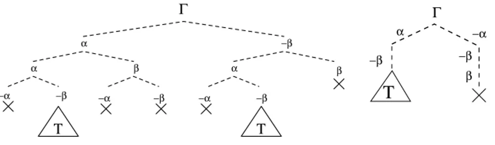
−β −β α −α βFig. 2. Search trees for the formula Γ = (α ∨ ¬β) ∧ (α ∨ β) ∧ (¬α ∨ ¬β). Left: a tableau-based procedure. Right: a DPLL-based procedure.
input formula, the propositional tableaux are used to enumerate up to all satis-fying assignments, which must be recursively checked for Km-consistency. This
requires checking recursively possibly-many sub-formulas of the formViαri∧¬βj
of depth d − 1, for which a propositional tableau will enumerate all satisfying assignments, and so on. At every level of nesting, a redundant truth assign-ment introduces a redundant modal search tree. Thus, with modal formulas, the redundancy of the propositional case propagates up-to-exponentially with the modal depth.
DPLL instead, performs a search which is based on semantic branching [24], i.e., a branching on the truth value of sub-formulas ψ of ϕ (typically atoms):4
ϕ
ϕ[ψ/>] ϕ[ψ/⊥],
where ϕ[ψ/>] is the result of substituting with > all occurrences of ψ in ϕ and then simplify the result. Thus, every branching step generates two mutually-inconsistent subtrees. Thus, DPLL always generates non-redundant sets of as-signments. This avoids search duplications and, in the case of modal search, the recursive exponential propagation of redundancy.
Example 2. Consider the formula Γ = (α∨¬β)∧(α∨β)∧(¬α∨¬β), where α and β are modal atoms s.t. α ∧ ¬β is Km-inconsistent, and let d be the depth of Γ .
The only assignment propositionally satisfying Γ is µ = α ∧ ¬β. Consider Figure 2, left. Two distinct but identical open branches are generated, both representing the assignment µ. Then the tableau expands the two open branches in the same way, until it generates two identical (and possibly-big) closed modal sub-trees T of modal depth d, each proving the Km-unsatisfiability of µ.
This phenomenon may repeat itself at the lower level in each sub-tree T , and so on. For instance, if α = 21((α0∨ ¬β0) ∧ (α0∨ β0)) and β = 21(α0∧ β0), then
at the lower level we have a formula Γ0 of depth d − 1 analogous to Γ . This
propagates exponentially the redundancy with the depth d.
4 Notice that the notion of “semantic branching” introduced in [24] is stronger than
that lately used in [27, 28]; the former coarsely corresponds to the latter plus the usage of unit-propagation.
−α −β −α −β −α −β α φ φ
T
T
1 1 2 2 β . . . . .T
3Γ
Γ
α −α −βT
23T
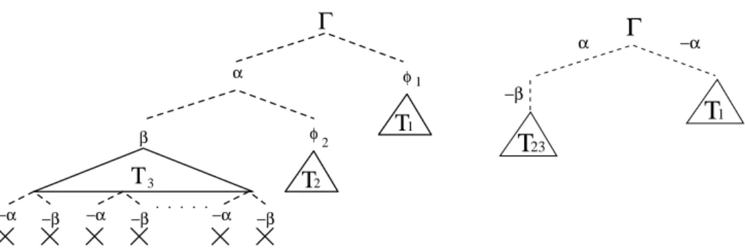
1Fig. 3. Search trees for the formula Γ = (α ∨ φ1) ∧ (β ∨ φ2) ∧ φ3∧ (¬α ∨ ¬β). Left: a
tableau-based procedure. Right: a DPLL-based procedure.
Finally, notice that if we considered the formula ΓK=VK
i=1(αi∨ ¬βi) ∧ (αi∨
βi) ∧ (¬αi∨ ¬βi), the tableau would generate 2K identical truth assignments
µK =V
iαi∧ ¬βi, and things would get exponentially worse.
Look at Figure 2, right. A DPLL-based procedure branches asserting α = > or α = ⊥. The first branch generates α ∧ ¬β, whilst the second gives ¬α ∧ ¬β ∧ β, which immediately closes. Therefore, only one instance of µ = α ∧ ¬β is generated. The same applies to µK.
Detecting constraint violations. A propositional formula ϕ can be seen as a set of constraints for the truth assignments which possibly satisfy it. For instance, a clause A1∨ A2 constrains every assignment not to set both A1 and A2 to ⊥.
Unlike tableaux, DPLL prunes a branch as soon as it violates some constraint of the input formula. (For instance, in Ksat this is done by the function assign.) Example 3. Consider the formula Γ = (α ∨ φ1) ∧ (β ∨ φ2) ∧ φ3∧ (¬α ∨ ¬β),
α and β being atoms, φ1, φ2 and φ3 being sub-formulas, such that α ∧ β ∧ φ3
is propositionally satisfiable and α ∧ φ2 is Km-unsatisfiable. Look at Figure 3,
left. Again, assume that, in a tableau-based procedure, the ∨-rule is applied in order, left to right. After two steps, the branch α, β is generated, which violates the constraint imposed by the last clause (¬α ∨ ¬β). A tableau-based procedure is not able to detect such a violation until it explicitly branches on that clause, that is, only after having generated the whole sub-tableau T3 for α ∧ β ∧ φ3,
which may be rather big. DPLL instead (Figure 3, right) avoids generating the violating assignment detects the violation and immediately prunes the branch.
3
Integrating DPLL and Theory Solvers: Lazy SMT
Satisfiability Modulo Theories is the problem of deciding the satisfiability of a first-order formula with respect to some decidable first-order theory T (SMT (T )). Examples of theories of interest are, those of Equality and Uninterpreted Func-tions (EUF), Linear Arithmetic (LA), both over the reals (LA(Q)) and the in-tegers (LA(Z)), its subclasses of Difference Logic (DL) and
Unit-Two-Variable-Per-Inequality (UT VPI), the theories of bit-vectors (BV), of arrays (AR) and of lists (LI).
Efficient SMT solvers have been developed in the last five years, called lazy SMT solvers, which combine DPLL with decision procedures (T -solvers) for many theories of interest (e.g., [1, 41, 15, 3, 4, 18, 19, 6, 16]).
3.1 Theory Solvers
In its simplest form, a Theory Solver for T (T -solver) is a procedure which takes as input a collection of T -literals µ and decides whether µ is T -satisfiable. In order to be effectively used within a lazy SMT solver, the following features of T -solver are often important or even essential.
Model generation: when T -solver is invoked on a T -consistent set µ, it is able to produce a T -model I witnessing the consistency of µ, i.e., I |=T µ.
Conflict set generation: when T -solver is invoked on a T -inconsistent set µ, it is able to produce the (possibly minimal) subset η of µ which has caused its inconsistency. η is called a theory conflict set of µ.
Incrementality: T -solver “remembers” its computation status from one call to the other, so that, whenever it is given in input a set µ1∪ µ2 such that µ1
has just been proved T -satisfiable, it avoids restarting the computation from scratch.
Backtrackability: it is possible for the T -solver to undo steps and return to a previous status on the stack in an efficient manner.
Deduction of unassigned literals: when T -solver is invoked on a T -consistent set µ, it can also perform a set of deductions in the form η |=T l, s.t. η ⊆ µ and
l is a literal on a not-yet-assigned atom in ϕ.
Deduction of interface equalities: when returning Sat, T -solver can also perform a set of deductions in the form µ |=T e (if T is convex) or µ |=T
W
jej (if
T is not convex) s.t. e, e1, ..., en are equalities between variables or terms
occurring in atoms in µ. We denote the equality (vi = vj) by eij, and we
call eij-deduction a deduction of (disjunctions of) eij’s. A T -solver is eij
-deduction-complete if it always capable to inferring the (disjunctions of) eij’s
which are entailed by the input set of literals. Notice that here the deduced equalities need not occur in the input formula ϕ.
3.2 Lazy Satisfiability Modulo Theories
We adopt the following terminology and notation. The bijective function T 2B (“theory-to-propositional”), called boolean abstraction, maps propositional vari-ables into themselves, ground T -atoms into fresh propositional varivari-ables, and is homomorphic w.r.t. boolean operators and set inclusion. The function B2T (“propositional-to-theory”), called refinement, is the inverse of T 2B. The sym-bols ϕ, ψ denote T -formulas, and µ, η denote sets of T -literals; ϕp, ψp denote
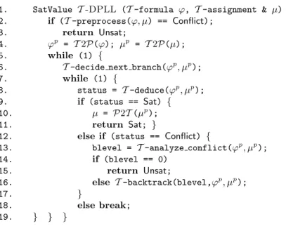
1. SatValue T -DPLL (T -formula ϕ, T -assignment & µ) { 2. if (T -preprocess(ϕ, µ) == Conflict);
3. return Unsat;
4. ϕp = T 2P(ϕ); µp = T 2P(µ);
5. while (1) {
6. T -decide next branch(ϕp, µp);
7. while (1) {
8. status = T -deduce(ϕp, µp);
9. if (status == Sat) {
10. µ = P2T (µp);
11. return Sat; }
12. else if (status == Conflict) {
13. blevel = T -analyze conflict(ϕp, µp);
14. if (blevel == 0) 15. return Unsat; 16. else T -backtrack(blevel,ϕp, µp); 17. } 18. else break; 19. } } }
Fig. 4. Schema of T -DPLL based on modern DPLL.
assignments) and we often use them as synonyms for the boolean abstraction of ϕ, ψ, µ, and η respectively, and vice versa (e.g., ϕp denotes T 2B(ϕ), µ denotes
B2T (µp)). If T 2B(ϕ) |= ⊥, then we say that ϕ is propositionally unsatisfiable,
written ϕ |=p⊥.
Figure 4 represent the schema of a T -DPLL procedure based on a modern DPLL engine. This schema evolved from that of the DPLL-based procedures for modal logics, see §2.2. The input ϕ and µ are a T -formula and a reference to an (initially empty) set of T -literals respectively. The DPLL solver embedded in T -DPLL reasons on and updates ϕp and µp, and T -DPLL maintains some
data structure encoding the set Lits(ϕ) and the bijective mapping T 2P/P2T on literals.
T -preprocess simplifies ϕ into a simpler formula, and updates µ if it is the case, so that to preserve the T -satisfiability of ϕ∧µ. If this process produces some conflict, then T -DPLL returns Unsat. T -preprocess combines most or all the boolean preprocessing steps for DPLL with some theory-dependent rewriting steps on the T -literals of ϕ. (The latter are described in §3.3.)
T -decide next branch selects the next literal like in standard DPLL (but it may consider also the semantics in T of the literals to select).
T -deduce, in its simplest version, behaves similarly to standard BCP in DPLL: it iteratively deduces boolean literals lpderiving propositionally from the
current assignment (i.e., s.t. ϕp∧ µp|= lp) and updates ϕp and µp accordingly,
(i) µp propositionally violates ϕp (µp∧ ϕp|= ⊥). If so, T -deduce behaves like
deduce in DPLL, returning Conflict.
(ii) µp propositionally satisfies ϕp (µp|= ϕp). If so, T -deduce invokes T -solver
on µ: if the latter returns Sat, then T -deduce returns Sat; otherwise, T -deduce returns Conflict.
(iii) no more literals can be deduced. If so, T -deduce returns Unknown. A slightly more elaborated version of T -deduce can invoke T -solver on µ at this intermediate stage: if T -solver returns Unsat, then T -deduce returns Conflict. (This enhancement, called early pruning, is discussed in §3.3.) A much more elaborated version of T -deduce can be implemented if T -solver is able to perform deductions of unassigned literals η |=T l s.t. η ⊆ µ, as in §3.1.
If so, T -deduce can iteratively deduce and propagate also the corresponding literal lp. (This enhancement, called T -propagation, is discussed in §3.3.)
T -analyze conflict is an extensions of analyze conflict of DPLL [42, 43]: if the conflict produced by T -deduce is caused by a boolean failure (case (i) above), then T -analyze conflict produces a boolean conflict set ηp and
the corresponding value of blevel; if the conflict is caused by a T -inconsistency revealed by T -solver (case (ii) or (iii) above), then T -analyze conflict pro-duces the boolean abstraction ηp of the theory conflict set η ⊆ µ produced
by T -solver, or computes a mixed boolean+theory conflict set by a backward-traversal of the implication graph starting from the conflicting clause ¬ηp (see
§3.3). Once the conflict set ηp and blevel have been computed, T -backtrack
behaves analogously to backtrack in DPLL: it adds the clause ¬ηp to ϕp,
ei-ther temporarily or permanently, and backtracks up to blevel. (These features, called T -backjumping and T -learning, are discussed in §3.3.)
T -DPLL differs from the standard DPLL [42, 43] because it exploits: – an extended notion of deduction of literals: not only boolean deduction (µp∧
ϕp|= lp), but also theory deduction (µ |= T l);
– an extended notion of conflict: not only boolean conflict (µp∧ ϕp |= p ⊥),
but also theory conflict (µ |=T ⊥), or even mixed boolean+theory conflict
((µ ∧ ϕ) |=T ⊥).
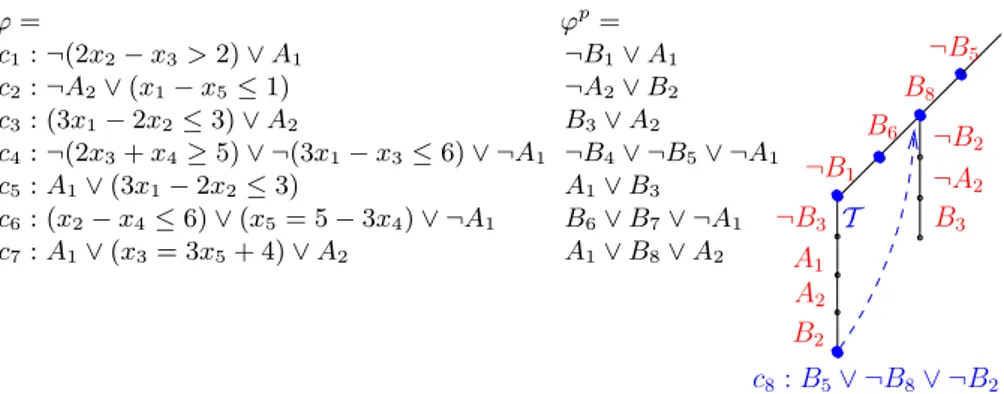
Example 4. Consider the LA(Q)-formulas ϕ and its boolean abstraction ϕp of
Figure 5. Suppose T -decide next branch selects, in order, µp:= {¬B
5, B8, B6, ¬B1}
(in c4, c7, c6, and c1). T -deduce cannot unit-propagate any literal. By the
en-hanced version of step (iii), it invokes T -solver on µ := {¬(3x1− x3≤ 6), (x3=
3x5+4), (x2−x4≤ 6), ¬(2x2−x3> 2)}. The enhanced T -solver not only returns
Sat, but also it deduces ¬(3x1− 2x2 ≤ 3) (c3 and c5) as a consequence of the
first and last literals. The corresponding boolean literal ¬B3, is added to µpand
propagated (T -propagation). Hence A1, A2and B2are unit-propagated from c5,
c3and c2.
Let µ0pbe the resulting assignment {¬B
5, B8, B6, ¬B1, ¬B3, A1, A2, B2}). By
step (iii), T -deduce invokes T -solver on µ0: {¬(3x
ϕ = ϕp= c1: ¬(2x2− x3> 2) ∨ A1 c2: ¬A2∨ (x1− x5≤ 1) c3: (3x1− 2x2≤ 3) ∨ A2 c4: ¬(2x3+ x4≥ 5) ∨ ¬(3x1− x3≤ 6) ∨ ¬A1 c5: A1∨ (3x1− 2x2≤ 3) c6: (x2− x4≤ 6) ∨ (x5= 5 − 3x4) ∨ ¬A1 c7: A1∨ (x3= 3x5+ 4) ∨ A2 ¬B1∨ A1 ¬A2∨ B2 B3∨ A2 ¬B4∨ ¬B5∨ ¬A1 A1∨ B3 B6∨ B7∨ ¬A1 A1∨ B8∨ A2 ¬B3 A1 A2 B2 ¬B2 ¬A2 B3 c8: B5∨ ¬B8∨ ¬B2 T ¬B5 B8 B6 ¬B1
Fig. 5. Boolean search (sub)tree in the scenario of Example 4. (A diagonal line, a ver-tical line and a verver-tical line tagged with “T ” denote literal selection, unit propagation and T -propagation respectively; a bullet “•” denotes a call to T -solver.)
x4 ≤ 6), ¬(2x2− x3 > 2), ¬(3x1− 2x2 ≤ 3), (x1− x5≤ 1)} which is
inconsis-tent because of the 1st, 2nd, and 6th literals, so that returns Unsat, and hence T -deduce returns Conflict. Then T -analyze conflict and T -backtrack learn the corresponding boolean conflict clause
c8=def B5∨ ¬B8∨ ¬B2
and backtrack, popping from µp all literals up to {¬B
5, B8}, and then
unit-propagate ¬B2 on c8 (T -backjumping and T -learning). Then, starting from
{¬B5, B8, ¬B2}, also ¬A2and B3are unit-propagated on c2and c3respectively.
As in standard DPLL, an excessive number of T -learned clauses may cause an explosion in size of ϕ. Thus, many lazy SMT tools introduce techniques for discharging T -learned clauses when necessary. Moreover, like in standard DPLL, T -DPLL can be restarted from scratch in order to avoid dead-end portions of the search space. The learned clauses prevent T -DPLL to redo the same steps twice. Most lazy SMT tools implement restarting mechanisms as well.
3.3 Enhancements
In the schema of Figure 4, even assuming that the DPLL engine and the T -solver are extremely efficient as a stand-alone procedures, their combination can be extremely inefficient. This is due to a couple of intrinsic problems.
– The DPLL engine assigns truth values to (the boolean abstraction of) T -atoms in a blind way, receiving no information from T -solver about their semantics. This may cause up to an huge amount of calls to T -solver on assignments which are obviously T -inconsistent, or whose T -inconsistency could have been easily derived from that of previously-checked assignments.
– The T -solver is used as a memory-less subroutine, in a master-slave fashion. Therefore T -solver may be called on assignments that are subsets of, super-sets of or similar to assignments it has already checked, with no chance of reusing previous computations.
Therefore, it is essential to improve the integration schema so that the DPLL solver is driven in its boolean search by T -dependent information provided by T -solver, whilst the latter is able to take benefit from information provided by the former, and it is given a chance of reusing previous computation.
We describe some of the most effective techniques which have been proposed in order to optimize the interaction between DPLL and T -solver. (We refer the reader to [36] for a much more extensive and detailed survey.) Some of them, like Normalizing T -atoms, Early pruning, T -backjumping and pure-literal filtering, derive from those developed in the context of DPLL-based procedures for modal logics.
Normalizing T -atoms. In order to avoid the generation of many trivially-unsatisfiable assignments, it is wise to preprocess T -atoms so that to map as many as possible T -equivalent literals into syntactically-identical ones. This can be achieved by applying some rewriting rules, like, e.g.:
– Drop dual operators: (x1< x2), (x1≥ x2) ⇒ ¬(x1≥ x2), (x1≥ x2).
– Exploit associativity: (x1+ (x2+ x3) = 1), ((x1+ x2) + x3) = 1) ⇒ (x1+
x2+ x3= 1).
– Sort: (x1+ x2− x3≤ 1), (x2+ x1− 1 ≤ x3) ⇒ (x1+ x2− x3≤ 1)).
– Exploit T -specific properties: (x1≤ 3), (x1< 4) ⇒ (x1≤ 3) if x1∈ Z.
The applicability and effectiveness of these mappings depends on the theory T .
Static learning. On some specific kind of problems, it is possible to quickly detect a priori short and “obviously T -inconsistent” assignments to T -atoms in Atoms(ϕ) (typically pairs or triplets). Some examples are:
– incompatible values (e.g., {x = 0, x = 1}),
– congruence constraints (e.g., {(x1= y1), (x2= y2), ¬(f (x1, x2) = f (y1, y2))}),
– transitivity constraints (e.g., {(x − y ≤ 2), (y − z ≤ 4), ¬(x − z ≤ 7)}), – equivalence constraints ({(x = y), (2x − 3z ≤ 3), ¬(2y − 3z ≤ 3)}).
If so, the clauses obtained by negating the assignments (e.g., ¬(x = 0)∨¬(x = 1)) can be added a priori to the formula before the search starts. Whenever all but one literals in the inconsistent assignment are assigned, the negation of the remaining literal is assigned deterministically by unit propagation, which prevents the solver generating any assignment which include the inconsistent one. This technique may significantly reduce the boolean search space, and hence the number of calls to T -solver, producing very relevant speed-ups [1, 6].
Intuitively, one can think to static learning as suggesting a priori some small and “obvious” T -valid lemmas relating some T -atoms of ϕ, which drive DPLL
in its boolean search. Notice that the clauses added by static learning refer only to atoms which already occur in the original formula, so that the boolean search space is not enlarged.
Early pruning. Another optimization, here generically called early pruning – EP, is to introduce an intermediate call to T -solver on intermediate assignment µ. (I.e., in the T -DPLL schema of Figure 4, this is represented by the “slightly more elaborated” version of step (iii) of T -deduce.) If T -solver(µ) returns Unsat, then all possible extensions of µ are unsatisfiable, so that T -DPLL returns Unsat and backtracks, avoiding a possibly big amount of useless search.
In general, EP may introduce a drastic reduction of the boolean search space, and hence of the number of calls to T -solvers. Unfortunately, as EP may cause useless calls to T -solver, the benefits of the pruning effect may be partly counter-balanced by the overhead introduced by the extra EP calls. To this extent, many different improvements to EP and strategies for interleaving calls to T -solvers and boolean reasoning steps [41, 19, 3, 6, 10] have been proposed.
T -propagation. As discussed in §3.1, for some theories it is possible to im-plement T -solver so that a call to T -solver(µ) returning Sat can also perform one or more deduction(s) in the form η |=T l, s.t. η ⊆ µ and l is a literal on an
unassigned atom in ϕ. If this is the case, then T -solver can return l to T -DPLL, so that lp is added to µp and unit-propagated [1, 3, 19]. This process, which is
called T -propagation, may induce a beneficial loop with unit-propagation. As with early-pruning, there are different strategies by which T -propagation can be interleaved with unit-propagation [1, 3, 19, 6, 10, 33].
Notice that T -solver can return the deduction(s) performed η |=T l to T
-DPLL, which can add the deduction clause (ηp→ lp) to ϕp, either temporarily
and permanently. The deduction clause will be used for the future boolean search, with benefits analogous to those of T -learning (see §3.3).
T -backjumping and T -learning. Modern implementations inherit the back-jumping mechanism of current DPLL tools: T -DPLL learns the conflict clause ¬ηp and backtracks to the highest point in the stack where one lp ∈ ηp is not
assigned, and unit propagates ¬lpon ¬ηp. Intuitively, DPLL backtracks to the
highest point where it would have done something different if it had known in advance the conflict clause ¬ηp from the T -solver.
As hinted in §3.2, it is possible to use either a theory conflict η (i.e., ¬η is a T -valid clause) or a mixed boolean+theory conflicts sets η0, i.e., s.t. an inconsistency
can be entailed from η0∧ ϕ by means of a combination of boolean and theory
reasoning ( η0∧ ϕ |=
T ⊥). Such conflict sets/clauses can be obtained starting
from the theory-conflicting clause ¬ηpby applying the backward-traversal of the
implication graph, until one of the standard conditions (e.g., 1UIP) is achieved. Notice that it is possible to learn both clauses ¬η and ¬η0.
Example 5. The scenario depicted in Example 4 represents a form of T -backjumping and T -learning, in which the conflict clause c8 used is a LA(Q)-conflict clause
(i.e., P2T (c8) is LA(Q)-valid). However, T -analyze conflict could instead
look for a mixed boolean+theory conflict clause by treating c8 as a conflicting
clause and backward-traversing the implication graph, that is, by resolving back-ward c8with c2and c3, (i.e., with the antecedent clauses of B2and A2) and with
the deduction clause c9 (which “caused” the propagation of ¬B3):
c8: theory conf licting clause
z }| { B5∨ ¬B8∨ ¬B2 c2 z }| { ¬A2∨ B2 B5∨ ¬B8∨ ¬A2 (B2) c3 z }| { B3∨ A2 B5∨ ¬B8∨ B3 (¬A2) c9 z }| { B5∨ B1∨ ¬B3 B5∨ ¬B8∨ B1 | {z } c0
8: mixed boolean+theory conf lict clause
(B3)
finding the mixed boolean+theory conflict clause c0
8 : B5∨ ¬B8∨ B1. (Notice
that, P2T (c0
8) = (3x1− x3≤ 6) ∨ ¬(x3= 3x5+ 4) ∨ (2x2− x3> 2) is not
LA(Q)-valid.) If so then T -backtrack pops from µp all literals up to {¬B
5, B8}, and
then unit-propagates B1on c08, and hence A1 on c1.
As with static learning, the clauses added by T -learning refer only to atoms which already occur in the original formula, so that no new atom is added. [18] proposed an interesting generalization of T -learning, in which learned clause may contain also new atoms. [7, 8] used a similar idea to improve the efficiency of Delayed Theory Combination (see §4).
Pure-literal filtering. If we have non-boolean T -atoms occurring only posi-tively [resp. negaposi-tively] in the input formula, we can safely drop every negative [resp. positive] occurrence of them from the assignment to be checked by T -solver [41, 22, 3, 6, 36].5 We call this technique, pure-literal filtering
There are two potential benefits for this behavior. Let µ0 be the reduced
version of µ. First, µ0 might be T -satisfiable despite µ is T -unsatisfiable. If so,
and if µ propositionally satisfies ϕ, then T -DPLL can stop, potentially saving a lot of search. Second, if µ0 (and hence µ) is T -unsatisfiable, then checking the
consistency of µ0 rather than that of µ can be faster and cause smaller conflict
sets, so that to improve the effectiveness of T -backjumping and T -learning. Moreover, this technique is particularly useful in some situations. For in-stance, many T -solvers for DL(Z) and LA(Z) cannot efficiently handle dise-qualities (e.g., (x1− x2 6= 3)), so that they are forced to split them into the
disjunction of strict inequalities (x1 − x2 > 3) ∨ (x1− x2 < 3). This causes
an enlargement of the search, because the two disjuncts must be investigated
5 If both T -propagation and pure-literal filtering are implemented, then the filtered
literals must be dropped not only from the assignment, but also from the list of literals which can be T -deduced, so that to avoid the T -propagation of literals which have already been filtered away.
separately. In many problems, however, it is very frequent that most equalities (t1= t2) occur with positive polarity only. If so, then pure-literal filtering avoids
adding (t16= t2) to µ when (t1 = t2)p is assigned to false by T -DPLL, so that
no split is needed [3].
4
DPLL for Theory Combination: DTC
We consider the SMT problem in the case of combined theories, SMT (T1∪
T2). In the original Nelson-Oppen method [31] and its variant due to Shostak
[38] (hereafter referred as deterministic N.O. 6) the two T -solvers cooperate by
inferring and exchanging equalities between shared terms (interface equalities), until either one T -solver detects unsatisfiability (Unsat case), or neither can perform any more entailment (Sat case). In case of a non-convex theory Ti,
the Ti-solver may generate a disjunction of interface equalities; consequently,
a Ti-solver receiving a disjunction of equalities from the other one is forced to
case-split on each disjunct. Deterministic N.O. requires that each T -solver is always capable to inferring the (disjunctions of) equalities which are entailed by the input set of literals (see §3.1). Whilst for some theories this feature can be implemented very efficiently (e.g., EUF [32]), for some others it can be extremely expensive (e.g., DL(Z) [30]).
Delayed Theory Combination ( Dtc) is a general method for tackling the problem of theory combination within the context of lazy SMT [7, 8]. As with N.O., we assume that T1, T2 are two signature-disjoint stably-infinite theories
with their respective Ti-solvers. Importantly, no assumption is made about the
eij-deduction capabilities of the Ti-solvers (§3.1): for each Ti-solver, every
inter-mediate situation from complete eij-deduction (like in deterministic N.O.) to no
eij-deduction capabilities (like in non-deterministic N.O.) is admitted.
In a nutshell, in Dtc the embedded DPLL engine not only enumerates truth assignments for the atoms of the input formula, but also assigns truth values for the interface equalities that the T -solver’s are not capable of inferring, and han-dles the case-split induced by the entailment of disjunctions of interface equalities in non-convex theories. The rationale is to exploit the full power of a modern DPLL engine by delegating to it part of the heavy reasoning effort previously due to the Ti-solvers.
An implementation of Dtc [8, 9] is based on the schema of Figure 4, ex-ploiting early pruning, T -propagation, T -backjumping and T -learning. Each of the two Ti-solvers interacts only with the DPLL engine by exchanging literals
via the truth assignment µ in a stack-based manner, so that there is no direct exchange of information between the Ti-solvers. Let T be T1∪ T2. The T -DPLL
algorithm is modified to the following extents [8, 9]:7
– T -DPLL must be instructed to assign truth values not only to the atoms in ϕ, but also to the interface equalities not occurring in ϕ. P2T and T 2P
6 We also call nondeterministic N.O. the non-deterministic variant of N.O. method
first presented in [34].
SAT!
and the consequent two branches
µ0
LA(Z)|=LA(Z)((v1= v3) ∨ (v1= v4))
Mimics the eij-deduction
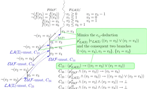
{¬(v1= v4), v1= v3}, {v1= v4} v1= v4 EUF-unsat, C14 C14: (µ000EUF∧ (v1= v3) ∧ (v2= v4)) → ⊥ v2= v4 EUF-unsat, C24 v2= v3 C24: (µ00EUF∧ (v1= v3) ∧ (v2= v3)) → ⊥ LA(Z)-unsat, C23 C23: (µ00LA(Z)∧ (v5= v6)) → ((v2= v3) ∨ (v2= v4)) ¬(v2= v4) ¬(v2= v3) v5= v6 EUF-unsat, C56 ¬(v5= v6) C56: (µ0EUF∧ (v1= v3)) → (v5= v6) v1= v3 LA(Z)-unsat, C13 ¬(v1= v4) ¬(v1= v3) C13: (µ0LA(Z)) → ((v1= v3) ∨ (v1= v4)) v5= v4− 1 v1≥ 0 v3= 0 v2≥ v6 v4= 1 v2≤ v6+ 1 v1≤ 1 µLA(Z): ¬(f (v1) = f (v2)) ¬(f (v2) = f (v4)) f (v3) = v5 f (v1) = v6 µEUF:
Fig. 6. The Dtc search tree for Example 6 on LA(Z) ∪ EUF, with no eij-deduction. v1, . . . , v6 are interface terms. µ0Ti, µ
00 Ti, µ
000
Ti denote generic subsets of µTi, T ∈
{EUF, LA(Z)}.
are modified accordingly. In particular, T -decide next branch is modified to select also new interface equalities not occurring in the original formula. – µp is partitioned into three components µp
T1, µ
p T2 and µ
p
e, s.t. µTi is the set
of i-pure literals and µeis the set of interface (dis)equalities in µ.
– T -deduce is modified to work as follows: for each Ti, µpTi∪ µ
p
e, is fed to the
respective Ti-solver. If both return Sat, then T -deduce returns Sat, otherwise
it returns Conflict.
– Early-pruning is performed; if some Ti-solver can deduce atoms or single
interface equalities, then T -propagation is performed. If one Ti-solver
per-forms the eij-deduction µ∗|=Ti
Wk
j=1ej, s.t. µ∗⊆ µTi∪ µe, each ej being an
interface equality, then the deduction clause T 2B(µ∗→Wk
j=1ej) is learned.
– T -analyze conflict and T -backtrack are modified so that to use the conflict set returned by one Ti-solver for T -backjumping and T -learning.
Importantly, such conflict sets may contain interface equalities.
In order to achieve efficiency, other heuristics and strategies have been further suggested in [7–9], and more recently in [17, 14].
Example 6. [9] Consider the set of EUF ∪ LA(Z)-literals µ =def µEUF∪ µLA(Z)
of Figure 6. We assume that both the EUF- and LA(Z)-solvers have no eij
-deduction capabilities (like with non-deterministic N.O.). For simplicity, we also assume that both Ti-solvers always return conflict sets which do not contain
is described in detail in [9].) In short, T -DPLL performs a boolean search on the eij’s, backjumping on the T -conflicting clauses C13, C56, C23, C24and C14,
which in the end causes the unit-propagation of (v1 = v4). Then, T -DPLL
selects a sequence of ¬eij’s without generating conflicts, and concludes that the
formula is T1∪ T2-satisfiable. Notice that the backjumping steps on the clauses
C13, C56, and C25mimic the effects of performing eij-deductions.
By adopting T -solvers with different eij-deduction power, one can trade part
or all the eij-deduction effort for extra boolean search. [9] shows that, if the
T -solvers have full eij-deduction capabilities, then no extra boolean search on
the eij’s is required; otherwise, the boolean search is controlled by the quality
of the conflict sets returned by the T -solvers: the more redundant ¬eij’s are
removed from the conflict sets, the more boolean branches are pruned. If the conflict sets do not contain redundant ¬eij’s, the extra effort is reduced to one
branch for each deduction saved, as in Example 6.
Variants of DTC are currently implemented in the MathSAT [8], Yices [17], and Z3 [14] lazy SMT tools.
4.1 Splitting on Demand
The idea of delegating to the DPLL engine part of the heavy reasoning effort previously due to the Ti-solvers is pushed even further in the Splitting on demand
technique proposed in [5]. This work is built on top of the observation that for many theories, in particular for non-convex ones, T -solvers must perform lots of internal case-splits in order to decide the satisfiability of a set of literals. Unfortunately most T -solvers cannot handle boolean search internally, so that they cannot do anything better then doing naive case-splitting on all possible combinations of the alternatives.
With splitting on demand, whenever the T -solver encounters the need of a case-split, it gives back the control to the DPLL engine by returning (the boolean abstraction of) a clause encoding the alternatives, which is learned and split upon by the DPLL engine. (Notice that the atoms encoding the alternatives in the learned clause may not occur in the original formula.) This is repeated until the T -solver can decide the T -satisfiability of its input literals without case-splitting. Therefore the T -solver delegates the boolean search induced by the case-splits to the DPLL solver, which presumably handles it in a much more efficient way.
References
1. A. Armando, C. Castellini, and E. Giunchiglia. SAT-based procedures for temporal reasoning. In Proc. European Conference on Planning, CP-99, 1999.
2. A. Armando and E. Giunchiglia. Embedding Complex Decision Procedures inside an Interactive Theorem Prover. Annals of Mathematics and Artificial Intelligence, 8(3–4):475–502, 1993.
3. G. Audemard, P. Bertoli, A. Cimatti, A. KorniÃlowicz, and R. Sebastiani. A SAT Based Approach for Solving Formulas over Boolean and Linear Mathematical Propositions. In Proc. CADE’2002., volume 2392 of LNAI. Springer, July 2002. 4. C. Barrett, D. Dill, and A. Stump. Checking Satisfiability of First-Order
For-mulas by Incremental Translation to SAT. In 14th International Conference on
Computer-Aided Verification, 2002.
5. C. Barrett, R. Nieuwenhuis, A. Oliveras, and C. Tinelli. Splitting on Demand in SAT Modulo Theories. In Proc. LPAR’06, volume 4246 of LNAI. Springer, 2006. 6. M. Bozzano, R. Bruttomesso, A. Cimatti, T. Junttila, P.van Rossum, S. Schulz, and
R. Sebastiani. MathSAT: A Tight Integration of SAT and Mathematical Decision Procedure. Journal of Automated Reasoning, 35(1-3), October 2005.
7. M. Bozzano, R. Bruttomesso, A. Cimatti, T. Junttila, P. van Rossum, S. Ranise, and R. Sebastiani. Efficient Satisfiability Modulo Theories via Delayed Theory Combination. In Proc. CAV 2005, volume 3576 of LNCS. Springer, 2005.
8. M. Bozzano, R. Bruttomesso, A. Cimatti, T. Junttila, P. van Rossum, S. Ranise, and R. Sebastiani. Efficient Theory Combination via Boolean Search. Information
and Computation, 204(10), 2006.
9. R. Bruttomesso, A. Cimatti, A. Franz´en, A. Griggio, and R. Sebastiani. Delayed Theory Combination vs. Nelson-Oppen for Satisfiability Modulo Theories: a Com-parative Analysis. In Proc. LPAR’06, volume 4246 of LNAI. Springer, 2006. 10. S. Cotton and O. Maler. Fast and Flexible Difference Logic Propagation for
DPLL(T). In Proc. SAT’06, volume 4121 of LNCS. Springer, 2006.
11. M. D’Agostino and M. Mondadori. The Taming of the Cut. Journal of Logic and
Computation, 4(3):285–319, 1994.
12. M. Davis, G. Longemann, and D. Loveland. A machine program for theorem proving. Journal of the ACM, 5(7), 1962.
13. M. Davis and H. Putnam. A computing procedure for quantification theory.
Jour-nal of the ACM, 7:201–215, 1960.
14. L. de Moura and N. Bjorner. Model-based Theory Combination. In Proc. 5th
workshop on Satisfiability Modulo Theories, SMT’07, 2007. To appear.
15. L. de Moura, H. Rueß, and M. Sorea. Lemmas on Demand for Satisfiability Solvers. Proc. SAT’02, 2002.
16. B. Dutertre and L. de Moura. A Fast Linear-Arithmetic Solver for DPLL(T). In
Proc. CAV’06, volume 4144 of LNCS. Springer, 2006.
17. B. Dutertre and L. de Moura. System Description: Yices 1.0. In Proc. on
2nd SMT competition, SMT-COMP’06, 2006. Available at yices.csl.sri.com/
yices-smtcomp06.pdf.
18. C. Flanagan, R. Joshi, X. Ou, and J. B. Saxe. Theorem Proving Using Lazy Proof Explication. In Proc. CAV 2003, LNCS. Springer, 2003.
19. H. Ganzinger, G. Hagen, R. Nieuwenhuis, A. Oliveras, and C. Tinelli. DPLL(T): Fast Decision Procedures. In Proc. CAV’04, volume 3114 of LNCS. Springer, 2004. 20. E. Giunchiglia, F. Giunchiglia, R. Sebastiani, and A. Tacchella. More evaluation
of decision procedures for modal logics. In Proc. KR’98, Trento, Italy, 1998. 21. E. Giunchiglia, F. Giunchiglia, R. Sebastiani, and A. Tacchella. SAT vs.
Transla-tion based decision procedures for modal logics: a comparative evaluaTransla-tion. Journal
of Applied Non-Classical Logics, 10(2):145–172, 2000.
22. E. Giunchiglia, F. Giunchiglia, and A. Tacchella. SAT Based Decision Procedures for Classical Modal Logics. Journal of Automated Reasoning. Special Issue: Satis-fiability at the start of the year 2000, 2001.
23. F. Giunchiglia and R. Sebastiani. Building decision procedures for modal logics from propositional decision procedures - the case study of modal K. In Proc.
CADE’13, LNAI, New Brunswick, NJ, USA, August 1996. Springer.
24. F. Giunchiglia and R. Sebastiani. A SAT-based decision procedure for ALC. In
Proc. KR’96, Cambridge, MA, USA, November 1996.
25. F. Giunchiglia and R. Sebastiani. Building decision procedures for modal logics from propositional decision procedures - the case study of modal K(m). Information
and Computation, 162(1/2), October/November 2000.
26. V. Haarslev and R. Moeller. RACER System Description. In Proc. of International
Joint Conference on Automated reasoning - IJCAR-2001, volume 2083 of LNAI,
Siena, Italy, July 2001. Springer-verlag.
27. I. Horrocks. Using an expressive description logic: FaCT or fiction? In Sixth
In-ternational Conference on Principles of Knowledge Representation and Reasoning (KR’98), pages 636–647, 1998.
28. I. Horrocks and P. F. Patel-Schneider. Optimizing Description Logic Subsumption.
Journal of Logic and Computation, 9(3):267–293, 1999.
29. I. Horrocks, P. F. Patel-Schneider, and R. Sebastiani. An Analysis of Empirical Testing for Modal Decision Procedures. Logic Journal of the IGPL, 8(3):293–323, May 2000.
30. S. K. Lahiri and M. Musuvathi. An Efficient Decision Procedure for UTVPI Con-straints. In Proc. of 5th International Workshop on Frontiers of Combining
Sys-tems (FroCos ’05), volume 3717 of LNCS. Springer, 2005.
31. G. Nelson and D.C. Oppen. Simplification by Cooperating Decision Procedures.
ACM Trans. on Programming Languages and Systems, 1(2):245–257, 1979.
32. R. Nieuwenhuis and A. Oliveras. Proof-Producing Congruence Closure. In
Pro-ceedings of the 16th International Conference on Term Rewriting and Applications, RTA’05, volume 3467 of LNCS. Springer, 2005.
33. R. Nieuwenhuis, A. Oliveras, and C. Tinelli. Solving SAT and SAT Modulo Theo-ries: from an Abstract Davis-Putnam-Logemann-Loveland Procedure to DPLL(T).
Journal of the ACM, 53(6):937–977, November 2006.
34. Derek C. Oppen. Complexity, convexity and combinations of theories. Theoretical
Computer Science, 12:291–302, 1980.
35. P. F. Patel-Schneider. DLP System Description. In Proc. Int. Workshop on
De-scription Logics, DL’98, 1998.
36. R. Sebastiani. Lazy Satisfiability Modulo Theories. Technical Report dtr-07-022, DIT, University of Trento, Italy, April 2007. Available at http://eprints.biblio. unitn.it/archive/00001196/01/dtr-07-022.pdf.
37. R. Sebastiani and A. Villafiorita. SAT-based decision procedures for normal modal logics: a theoretical framework. In Proc. AIMSA’98, volume 1480 of LNAI. Springer, 1998.
38. R.E. Shostak. Deciding Combinations of Theories. Journal of the ACM, 31:1–12, 1984.
39. R. M. Smullyan. First-Order Logic. Springer-Verlag, NY, 1968.
40. C. Tinelli. A DPLL-based Calculus for Ground Satisfiability Modulo Theories. In
Proc. JELIA-02, volume 2424 of LNAI, pages 308–319. Springer, 2002.
41. S. Wolfman and D. Weld. The LPSAT Engine & its Application to Resource Planning. In Proc. IJCAI, 1999.
42. L. Zhang, C. F. Madigan, M. W. Moskewicz, and S. Malik. Efficient conflict driven learning in boolean satisfiability solver. In ICCAD, pages 279–285, 2001.
43. L. Zhang and S. Malik. The quest for efficient boolean satisfiability solvers. In