UNIVERSITY
OF TRENTO
DIPARTIMENTO DI INGEGNERIA E SCIENZA DELL’INFORMAZIONE
38123 Povo – Trento (Italy), Via Sommarive 14
http://www.disi.unitn.it
TIME-DOMAIN INVERSION WITH THE IMSA-FBTS APPROACH
L. Manica, G. Oliveri, T. Takenaka, K. Hong-Ping, T. Moriyama, and A.
Massa
January 2011
Time‐Domain Inversion with the IMSA‐FBTS Approach
L. Manica1,2, G. Oliveri1, T. Takenaka2, K. Hong‐Ping2, T. Moriyama2, and A. Massa1
1 ELEDIA Group ‐ Department of Information Engineering and Computer Science Trento University, via Sommarive 14, I‐38050 Trento, Italy
[email protected], [email protected], [email protected]
2 Department of Electrical and Electronic Engineering Nagasaki University, 852‐8521 Japan
takenaka@nagasaki‐u.ac.jp, [email protected], t‐moriya@nagasaki‐u.ac.jp
Abstract: In this paper, the problem of localization, shaping, and reconstructing the dielectric
permittivity of a dielectric target is addressed. The inversion technique processes the time‐ domain scattered field data to reconstruct with an increasing degree of accuracy the unknown scatterer by exploiting an iterative multiscaling procedure. Preliminary numerical results are presented to validate the time‐domain multi‐resolution multi‐step approach.
Keywords: Microwave Imaging, Forward‐Backward Time‐Stepping Method, Iterative
Multiscaling Method.
1. Introduction
Microwave imaging techniques based on inverse‐scattering methodologies are aimed at localizing and reconstructing the dielectric properties of unknown scatterers from the measurement of the scattered field. An inverse scattering problem is usually very difficult because its nonlinearity, the ill‐posedness, and the non‐uniqueness of the solution [1]. Several inversion methods have been proposed in the frequency‐domain by assuming a monochromatic illumination of the scenario under test [2‐3]. Although frequency‐based techniques have been successfully applied in different applicative domains (e.g., medical imaging and nondestructive testing) with satisfactory results [4‐6], they present some drawbacks. More specifically, the use of higher frequencies enables an improvement of the spatial resolution achievable from the inversion, but it leads to a highly nonlinear formulation and a growing complexity in measuring the phase of the scattered field. On the other hand, the exploitation of single‐frequency data only allows the collection of a limited amount of information. To properly address these issues, multiple acquisitions at different frequencies are necessary [7] or broadband probing fields should be adopted [8‐9]. This latter is usually preferred even if it requires a time‐domain field analysis with a non negligible computational burden (i.e., storage resources and computational time). As a matter of fact, the numerical solution of the inverse problem at hand needs the discretization of both the investigation domain (i.e., the area where the unknown scatters are located) and the region surrounding the transmitters and the receivers [10].
To limit the computational burden of time‐domain inversions as well as enhance the spatial resolution, this work presents an innovative approach based on the time‐domain application of the iterative multiscaling methodology [11].
The outline of the paper is as follows. Section 2 is devoted to the mathematical formulation of the time‐domain inverse scattering problem and the IMSA solution is presented. Successively (Sect. 3), a representative test case is discussed to preliminary validate the proposed approach. Finally (Sect. 4), some conclusions are drawn and future developments envisaged. 2. Mathematical Formulation Let us consider a two‐dimensional unknown scatterer belonging to an investigation domain . The scatterer is illuminated successively by short pulses waves generated by a set of sources located at . The scattered field is collected at
inv D V
(
v , , ,V rt v =12K)
M different ( )v measurement points r(
12 (v))
m m , , ,M r = K placed in an observation domain enclosing the investigation domain. The material properties of the scatterer are modeled by means of a parameter vector function obs D(
x,y τ)
defined as( )
x,y[
ε( )
x,y σ( )
x,y]
τ = r −1; (1) where and are the dielectric permittivity and electric conductivity of the scatterer, respectively. The background medium is assumed to be free space.( )
x,yεr σ
( )
x,yAs far as the multi‐scaling procedure is concerned, it is applied as follows. At the initialization step ( ), a “coarse” profile of the object function is reconstructed by applying the Forward‐ Backward Time Step (FBTS) algorithm [9]. Towards this end, the investigation domain is discretized into cells of size 0 = s ) 0 ( inv D N Δx =ΔΔ =L( )/ N inv ) ( inv ) ( inv0 0 0 and the profile of the object function is retrieved by minimizing of the following cost function [9]:
( )
(
)
∫
∑∑
( )
(
( )
)
( )
0 1 1 2 ) ( ) ( ) ( 0 ~ T V v M m t v m t v s m mv s v s ; t, r E -t, r ; y x, τ E t K y x, τ Q = = = = (2)where E~m
( )
rvt,t is the measured electric field at the receiver positions due to the pulse radiated by the source located at th m t v r(
v=1,2,K,V)
and E(
τ( )
x,y ;rt t,)
v s m ) ( is the field due to the parameter vector function estimated at the s‐th step, τ(s)( )
x,y . The weighting factor Kmv( )
t is a nonnegative function which takes the value of zero at t= , T being the time duration of the T measurement. The estimated dielectric profile is processed to determine a reduced investigation domain (called “Region‐of‐Interest”) as described in [11][12]. Again, the reconstruction is carried out by means of the FBTS now considering a finer spatial grid. The iterative procedure is repeated until stationary conditions hold true [13]. ) 1 ( inv D 3. Numerical Assessment In order to validate the proposed approach, let us consider the reconstruction of a dielectric hollow square cylinder centered in (0.05,0.05)[m with] a relative permittivity equal to εr =2.0. r side of the cylinder has dimension 0.09 m , [ ] e inner side is equal to 0.03[m] vely [Fig. 2(a)]. Sixteen transmitters and sixteen receivers have been located at equally spaced points on a circle of radius R 0.5[ The oute while th respecti ] m = around Hz and ba has be ith a p . The initia Figures 2(c)‐2(e) show the evolution of the reconstruction throughout the iterative multiscaling the object. A band‐pass Gaussian incident pulse with center frequency f0=2[G nd‐width 1 GHz.3[ en adopted for the illumination. The time duration T of the measurement has been set to 217Δt w me step size of Δt=93.74 l guess solution has been chosen equal to the free‐space [Fig. 2(b)]. ] ] ti sec] [approach. At the initial step (s=0), the investigation domain is sized as follows ] [ 0.25 ] 0.25[ ) 0 ( (0) L m m
Linv× inv = × and it has been discretized into N =25 cells. After the FBTS has been roughly localized at (0.04 )[m [Fig. 2(c)] and a ] Region‐of‐Interest of size (1) (1) 0.15[ ] 0.15[ ]
inv L m m
L × inv = × and cen
reconstruction, the scatterer 4,0.044
ter
(
)
(0.04,0.04)[m] has been determine the = y , x (1) c ) 1 ( cd. At successive step (s=1), the retrieved object rofil own 2(d). At the stationary con Fig.
p e is sh in Fig. dition of the IMSA, the final result shown in 2(e) has been reached. (a) (b) (c) (d) (e) (f)
igure 2. (a) Hollow dielectric square cylinder (true object), (b) Initial guess for both “bare” – F
IMSA, (c) reconstruction after the 1st IMSA step, (d) reconstruction after the 2nd IMSA step, (e) reconstruction after the 3rd IMSA step (final result) and (f) reconstruction of the “bare” approach.
In order to point out the effectiveness and reliability of the proposed approach, the solution has
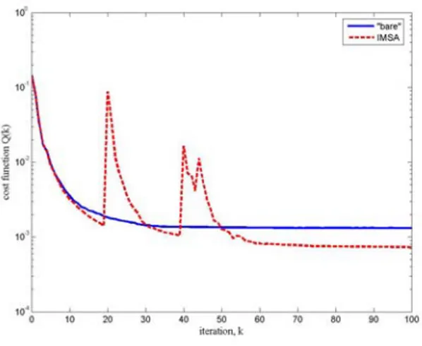
For completeness, the evolution of the
been compared with that obtained with the “bare” FBTS approach [Fig. 2(f)]. In such a strategy, a uniform discretization, equal the finest spatial resolution achieved with the IMSA, has been chosen within the whole investigation domain. As expected, although the “bare” method correctly locates the scatterer, the IMSA performs a better reconstruction of the unknown object.
cost function during the iterative minimization is reported in Fig. 3 for both the IMSA and the “bare” approach. As regards the computational costs, Table I summarizes the obtained results. The number of iterations to achieve the convergence, the total amount of time,
tot
T , the average time t for each
tion, and the number f cells N used to discretize the investigati domain ar reported. The computational indexes confirm that the IMSA
outperforms the “bare” ap oach ith a
itera o on e pr reduction w Figure 3. Cost function evolution.
of the computational time of about 31 (2 b. I
288 sec vs. 3301 sec – Tab. I) and of the complexity of about ½ (25 cells vs. 64 cells – Ta ) “Bare” FBTS IMSA – FBTS Step No. ‐ 0 1 2 ‐ Iterations 100 20 20 60 100 [sec] tot T 3301.82 306.94 335.58 1646.29 2288.81 [sec] t 33.02 15.35 16.77 27.44 22.89 N 64 25 25 25
Table I. Computational indexes.
4. Conclusions
In this paper, a procedure based f the iterative multiscaling approach and
References
1 D. Colton and R. Kress, Inverse Acousti magnetic Scattering Theory, Springler‐
Van den Berg, “A modified gradient method for two‐dimensional on the integration o
the forward‐backward time‐stepping algorithm has been presented to address the inversion of time‐domain data. Selected numerical results confirm, although in a preliminary fashion, the effectiveness and efficiency of the proposed reconstruction strategy. As a matter of fact, the method reduces the computational burden, decreasing both the storage resources and the time needed to perform the inversion, enabling a more detailed retrieval of the scatterer properties. However, further and deeper analyses are mandatory to assess in a more exhaustive way both features and limitations of the time‐domain multi‐resolution technique. c and Electro Verlag, New York, 1992. 2 R. E. Kleiman and P. M.
3 W. C. Chew and Y. M. Wang, “Reconstruction of two‐dimensional permittivity distribution
ceschini, M. Raffetto, M. Pastorino, and M. Donelli,
ed on a particle swarm optimizer
ch for microwave imaging of large
on and W.C. Chew, “Time‐domain inverse scattering using the local shape inverse scattering
ger, “A perfectly matched layer for the absorption of electromagnetic waves,” J.
w methodology based on
tection, location and imaging of multiple
integrated multi‐scaling
using the distorted Born iterative method,” IEEE Trans. Med. Imag., Vol. 9, no. 2, June 1990. 4 S. Caorsi, A. Massa and M. Pastorino, “A computational technique based on a real‐coded
genetic algorithm for microwave imaging purposes,” IEEE Trans. Geosci. Remote Sens., Vol. 38, no. 4, pp. 1697‐1708, July 2000.
5 A. Massa, D. Franceschini, G. Fran
“Parallel GA‐based approach for microwave imaging applications,” IEEE Trans. Antennas
Propagat., Vol. 53, no. 10, pp. 3118‐3127, October 2005.
6 M Donelli and A. Massa, “A computational approach bas
for microwave imaging of two‐dimensional dielectric scatterers,” IEEE Trans. Microwave
Theory Techn., Vol. 53, no. 5, pp. 1761‐1776, May 2005.
7 W. C. Chew and J.‐H. Lin, “A frequency‐hopping approa
inhomogeneous bodies,” IEEE Microwave Guided Wave Lett., Vol. 5, no. 12, pp. 439‐441, Dec. 1995. 8 W. H. Weld function (LSF) method,” Inverse Problems, Vol. 9, pp. 551‐564, Oct. 1993. 9 T. Tanaka, T. Takenaka, and S. He, “An FDTD approach to the time‐domain for an inhomogeneous cylindrical object,” Microwave Opt. Tech. Lett., Vol. 20, no. 1, pp. 72‐ 77, 1999. 10 J. P. Beren Computational Physics, Vol. 114, no. 2, pp. 185‐200, Apr. 1994.