CONSIDERING GROUPS IN THE STATISTICAL MODELING OF SPATIO-TEMPORAL DATA
D. Cocchi, F. Bruno
1. INTRODUCTION
Modern statistics is progressively dealing with data that do not come from in-dependent, identically distributed random processes. Spatially organized data are a peculiar example of this situation. Different forms of spatial data are available, which has led to the development of alternative modeling techniques. The com-monly used classification of spatial data was proposed by Cressie (1993) and dis-tinguishes data types according to the nature of the spatial domain under study. If it is fixed (i.e., non random), it is possible to discriminate between continuous and discrete domains, which lead, respectively, to geostatistical and lattice data. In these cases, the data-generating process corresponds to a collection of random variables (univariate/multivariate and continuous/discrete) over the domain. When the domain is random (i.e., the observed locations are the realization of an underlying process), the statistical investigation concerns spatial point patterns. Observing a variable at each point is not necessary for studying such a process because the data-generating process essentially defines the realizations of a point in the domain. When a variable is observed in the realization of a point process, however, the reference is to marked spatial point patterns. Many peculiar features of the three kinds of data are described, for example, in Gaetan and Guyon (2010).
When the data have both spatial and temporal dimensions, the categories de-scribed above can be organized in a spatio-temporal framework. The literature on spatio-temporal models is extensive, both in theory and in application. Spatio-temporal point processes are managed with specific tools. Examples include measures of intensity and second-order properties concerning the interaction among points in the domain estimated by non-parametric techniques (see, for ex-ample, Diggle, 1983; Adelfio et al., 2009).
Theoretical developments for spatio-temporal data in non-random domains can be classified according to different approaches: the geostatistical approach, which is based essentially on the specification of a covariance structure (see, for example, Christakos, 2000, and Gneiting et al., 2007); model-based formalizations,
such as hierarchical models developed under Bayesian or likelihood paradigms (see Banerjee et al., 2004, and Finkenstadt et al., 2007); and composite strategies (useful when computational issues seriously limit the use of models) that consist of multi-step procedures combining several complementary tools and models (see Jona Lasinio et al., 2007, and Pollice and Jona Lasinio, 2009, 2010).
For lattice spatio-temporal data, important literature associated with disease-mapping modeling is available. The two most popular approaches are the spatio-temporal mixture model proposed in Bohning (2003) and the Bayesian model suggested by Bernardinelli et al. (1995). The first approach develops a Poisson mixture model under a hierarchical perspective, and the second models both area-specific intercepts and temporal trends as random effects. The second formula-tion also allows for spatio-temporal interacformula-tions when the temporal risk trends vary by spatial locations and a spatial structure may be detected. This situation is usually addressed via CAR models. Univariate CAR models were extended to the multivariate case under the Bayesian viewpoint in Greco and Trivisano (2009).
Hierarchical models are frequently adopted for both continuous and discrete spatial domains. They are flexible and permit, by means of a sequence of condi-tional models, separation of the different sources of uncertainty. These models can be adopted in many different situations. The earliest proposed hierarchical model in the spatio-temporal context dealt with the normal case (Wikle et al., 1998). Non-normality has been subsequently addressed; for example, Sang and Gelfand (2009) modeled extreme value events, such as rainfall, for which the generalized extreme value (GEV) distribution is included in the hierarchy.
Geostatistical data and lattice data share similar assumptions regarding ran-domness. In the following, we expand the framework for studying these data by considering the inclusion of domain classifications with respect to certain differ-entiating features (Wang et al., 2009). When studying air pollution, for example, monitoring stations may be differently located with respect to traffic or house-hold density (Bruno and Cocchi, 2006). This peculiarity can be modeled in a number of different ways. In this work, we describe and compare some methods for incorporating the presence of subgroups in model building, with special em-phasis on Bayesian modeling. The paper is organized as follows. Section 2 intro-duces the main assumptions of geostatistical spatio-temporal processes. Section 3 describes the characteristics of spatio-temporal hierarchical models. Section 4 il-lustrates how differences in spatial locations can enter into a hierarchical model, and such a model is tested by simulations in Section 5. Section 6 contains some concluding remarks.
2. THE MAIN ASSUMPTIONS FOR MODELING SPATIO-TEMPORAL DATA UNDER THE GEO-STATISTICAL APPROACH
Inference on spatitemporal data is usually based on a model constructed o-ver single observations, as it is for the separate spatial or temporal cases. It is nec-essary to state some basic assumptions. Because the spatio-temporal domain is a
combination of the spatial and temporal ones, the usual assumptions of stationar-ity and isotropy of spatial statistics have to be directly extended. Subsequent as-sumptions about the joint consideration of space and time, such as separability and full symmetry, are often made to simplify computations in the model estima-tion. In the last two decades, the need for flexible models of space-time covari-ance functions that take these assumptions into account has emerged. The con-trasts between stationarity and non-stationarity, between full symmetry and only temporal asymmetry and between spatial isotropy and anisotropy can be high-lighted by suitably constructed space-time covariance functions.
Among the peculiarities mentioned above, the concept of non-separability ne-eds to be deepened. A spatio-temporal process is said to be non-separable if its spatio-temporal covariance function cannot be obtained as the sum or the prod-uct of a spatial covariance function and a temporal covariance function. This fea-ture has been ignored for quite some time, probably for computational reasons. In the earliest models, a space-time covariance function was defined as a product of a time and a space component. In the late 1990s, Cressie and Huang (1999) proposed a spectral approach for dealing with non-separable covariance functions of a general class that includes the covariance function expressed as the separated sum of a spatial and a temporal component as a special case (De Cesare et al., 2001). Successively, Gneiting (2002) has developed a Fourier-free approach for defining non-separable spatio-temporal covariance functions as combinations of a completely monotone function and a function whose first derivative is com-pletely monotone. Porcu et al. (2006) have proposed a generalization of Gneit-ing’s approach via a new class of stationary, non-separable spatio-temporal co-variance functions that are spatially anisotropic. Further contributions addressing particular features of non-separability are found in Ma (2002), Stein (2005) and Fernandez-Casal et al. (2003).
Testing non-separability has been the major feature of a few proposed models. Fuentes (2006) has constructed an analysis of variance-type test under a spectral approach, and Lu and Zimmerman (2005) and Mitchell et al. (2006) have pro-posed a likelihood-ratio test for separable covariance matrices that considers the decomposition of the covariance matrix via a Kronecker product. Li et al. (2007) have tested the usual assumptions on the space-time covariance functions via the asymptotic normality of the covariance estimators. Recently, Crujeiras et al. (2010) have proposed a test statistic based on a representation of the logarithm of the periodogram as the response variable in a regression model, assuming an additive form of the model under the assumption of separability.
The other typical spatio-temporal assumption on the covariance function is full symmetry. A spatio-temporal covariance function is said to be fully symmetric if it is symmetric with respect to the temporal dimension (Gneiting et al., 2007). Se-parability is a special case of full symmetry. Stationary space-time covariance fun-ctions that are not fully symmetric can be constructed on the basis of diffusion equations or stochastic partial differential equations. A series of related problems have been discussed by Jones and Zhang (1997), Brown et al. (2000), Kolovos et al. (2004) and Jun and Stein (2004).
Given the above premises, the basic formalization can now be sketched. Let { ( , );( , )Z t t Rd R}
Z u u
be the most general description of a spatio-temporal process. Usually, it is ex-pressed as
( , ) m( , ) w( , )
Z u t u t u t , (1)
where m( , )u t is a large-scale component that often denotes a trend and w( , )u t is a small-scale component with null expectation that captures the randomness of the spatio-temporal process. The analysis of a spatio-temporal process may have different focuses. For spatio-temporal trend detection (Kyriakidis and Journel, 1999), attention is on the first component, which defines the expected value of the process. For prediction, the focus is on the second component, which con-tains all the information about the spatio-temporal covariance or correlation function.
The large scale component can be modeled in a variety of ways; the options al-lowed by linearity are exploited first. A general expression in this case is
m( , )u t x u( , )' ( , )t β u t , (2)
where ( , )x u t is for a generic location and time ( , )ut the p-dimensional vector of spatio-temporal covariates, when available. Without covariates, ( , )x u t reduces to the p-dimensional vector of unit values. In the above expression, the choice of
( , )t
β u among the simpler β , ( )β t and ( )β u or the full ( , )β u t depends on the characteristics of the trend and covariates. The choice of a common space-time parameter β can be justified by the search for a parsimonious model (Cocchi et al., 2007). Time-varying coefficient models according to ( )βt are described in Lee and Shaddick (2007), and the case employing ( )β u is known as geographically weighted regression (Fotheringham et al., 1998).
The spatio-temporal process ( , )Z u t defined in (1) can be expressed as a hier-archical model, as illustrated in the next section.
3. HIERARCHICAL MODELS FOR SPATIO-TEMPORAL DATA
Hierarchical models provide a coherent probabilistic framework in which to incorporate, explicitly in the model, the uncertainty related to judgment, scientific reasoning, subjective decisions and experience. Hierarchical modeling relies on the joint distribution of a collection of random variables that can be decomposed into a series of conditional models (Gelman et al., 2004). These models can be considered from either a classical or a Bayesian perspective. The latter viewpoint may become necessary when the level of complexity increases (or when “subjec-tive” prior information is included).
For a general process, the idea is to approach the problem by breaking it into three basic stages, where [ | ] represents a conditional density probability func-tion (e.g., Wikle et al. 1998):
stage 1. Data Model: [data|process; parameters] stage 2. Process Model: [process|parameters] stage 3. Parameter Model: [parameters].
The first stage concerns the observational process (or the measurement error), and specifies the distribution of the data given the process of interest and certain relevant parameters. The second stage describes the underlying process, condi-tional on other parameters. Finally, the last stage accounts for the uncertainty in the parameters and is genuinely Bayesian.
The inference involves the joint distribution of the process and parameters that are updated by the data, and Bayes’ rule allows obtaining the posterior distri-bution, which may be factorized as follows:
[proc.;param.|data]~[data|proc.;param.][proc.|param.][param.].
This factorization of the posterior density is fundamental for constructing inter-pretable results.
Hierarchical models are useful in the spatio-temporal context, given the diffi-culty of specifying joint multivariate spatio-temporal covariance structures. Spa-tio-temporal processes are in fact characterized by a range of spatial and temporal scales of variability that include nonlinear interactions across domains and vari-ables. Wikle (2003) provides a detailed description of spatio-temporal hierarchical models for environmental studies. For a spatio-temporal process, a joint distribu-tion describes the stochastic behavior of the process at all spatial locadistribu-tions and all times, including all possible interactions between time and space. Such a distribu-tion is often difficult to construct. Hence, a more manageable alternative soludistribu-tion specifies the distribution of the relevant conditional models, bearing in mind that hierarchical models can often be seen as versions of variance components models (Zaslavsky, 2003).
The stages of the hierarchical model described above are now tailored for spa-tio-temporal modeling (see, for example, Wikle, 2003). A basic example is now illustrated, highlighting the common features.
If ( , )Y u t denotes data for the generic location and time (u,t), the entire data set can be expressed through the Tn-dimensional vector (Banerjee et al., 2004)
1
{ ( , ); ( ,...,Y t n), (1,..., )}t T
Y u u u u .
Let θ represent a collection of model parameters. These parameters conceptu-ally refer to the different stages in which the hierarchical model is structured and are therefore endowed with a subscript indicating the stage.
proc-ess. The simplest proposal considers Y as the sum of Z , the latent Tn-dimensional process of interest, and a zero mean measurement error ε :
Y Z ε . (3) In terms of conditionally independent distributions, it can be specified as
1
[ | , ]Y Z θ , (4)
where θ is the vector of parameters of the first stage, usually related to the dis-1 tribution of ε , and Z is the spatio-temporal process to be modeled in the further stages. The measurement error is defined at this stage; it is contained in the vari-ance component.
The second stage permits modeling of the spatio-temporal process as a whole. It allows highlighting all of the spatio-temporal characteristics, such as the exis-tence of a large-scale process or specific sub-processes. In the latter case, the dis-tribution is often further hierarchically factorized into a series of conditionally in-dependent submodels. The spatio-temporal process, described in the previous section, can be reformulated as a combination of a large-scale, or trend, spatio-temporal process ( m ) and a small scale process ( w ) that represents the spatial effects in time:
Z m w , (5) where both m and w are Tn-dimensional vectors. This formulation is the most
critical step in constructing the hierarchical model. In terms of conditional distri-butions, it can also be specified as
2
[ | , ]Z m θ , (6)
where θ is the vector of parameters at the second stage. 2
The third stage specifies priors for all the model parameters (θ and 1 θ , in this 2 case). This specification can involve hyperparameters denoted by θ . As in the 3 case of data and process modeling, the distribution of the parameters can be par-titioned into a series of distributions. It is convenient to assume a partition into hyperparameters, θ3(θ3 1 ,θ3 2 ), with respect to each stage and to state condi-tional independence relationships, such as [ , | ] [ |θ θ θ1 2 3 θ θ1 3 1 ][ |θ θ2 3 2 ]. To complete the hierarchy, a final fourth stage of the hierarchical model may contain further priors on the hyperparameters.
In the presence of many sub-processes, the number of stages for the final specification of the Bayesian hierarchy can increase.
3.1 The special Gaussian case
The Gaussian case, due to (4), assumes that, conditionally on Z and θ , the 1 ( , )
Y u t ’s are mutually independent with 2 ( , ) ( ( , ), ( , )) Y u t N Z u t u t . Hence, 2 1{ ( , ); ( ,..., t 1 n), (1,..., )}t T θ u u u u
is the set of spatio-temporal variances of the first-stage data model, where the re-sidual variances of the measurement process are isolated.
At the second stage, according to (6), Z follows the distribution [ | , ]~ ( , )Z m θ2 N m θ , where 2 θ is the collection of second stage parameters and 2 m is to be duely specified.
4. SPATIO-TEMPORAL MODELING FOR GROUPED POPULATIONS
Grouping can result from differences in spatial means and/or spatial variations in structure. In addition to territorial differences, it may derive from particular features, such as the structural characteristics of the spatial locations or the spe-cific covariate values that can lead to homogeneous groups with respect to the spatial means and/or correlation structure. Homogeneous groups may share a common spatial domain.
Models that allow for differences between groups of sites have recently been proposed; in environmental applications, for example, the different specifications are motivated by the nature of data rather than by a general theory. Cocchi et al. (2006), for example, have proposed a hierarchical spatio-temporal model for the daily mean concentrations of PM10 pollution. The main aim in this model is the identification of the sources of variability characterizing the PM10 diffusion and the estimation of the pollution levels at unmonitored locations. In this work, the group differences were captured by the intercept of the model, which translates the difference in pollution levels between the urban and rural locations. In Paci (2010), a spatio-temporal hierarchical model for Ozone in the Emilia Romagna region was proposed for data that again referred to urban and rural locations. The work compared group-specific temporal models using a unified spatio-temporal model that incorporated both types in the hierarchy. In the unified model, the differences between the groups of locations were captured by the mean (i.e., the trend component).
Another contribution that allows for including differences in locations due to groups is Sahu and Nicolis (2009). In this paper, PM data measured by two dif-ferent instruments (LVG and TEOM) are hierarchically modeled to achieve cali-bration. Moreover, Sahu et al. (2007) have proposed a hierarchical space-time
model for PM that includes two spatio-temporal processes; the first captures the background effects, and the second adds extra variability for urban locations by using the relationship between the response variable and suitable covariates (the population density, in this case).
We think that the inclusion of groups in spatio-temporal models needs to be formalized in a more general way. For this reason, we describe alternative pro-posals for including group differences in hierarchical Bayesian models in this sec-tion. The assessment of the consequences for spatial prediction under this inno-vation will be also considered.
When an overall model is proposed for a spatio-temporal process, its trend component may hide group-specific differences (Cressie, 1998). To avoid incor-rect forecasts, group-specific parameters should be included in the model. Hierar-chical models, being very flexible, are suitable for dealing with differences both at the measurement and the process level.
When group-specific models, or overall models that do not admit correlation between groups, are adopted, a lack of information is postulated that might be corrected by a more appropriate model construction. Introducing parameters that are capable of modeling beyond an elementary spatial structure ought to give bet-ter predictions.
We now describe the basic hierarchical model in this framework, with an em-phasis on the Gaussian case.
First, we specify the structure of the model sketched in Section 3, starting from the first-level specification (3) in which all of the components of the vector
1
{ ( , ); ( ,..., t n), (1,..., )}t T
ε u u u u follow i.i.d. Gaussian distributions. In
terms of the conditional distributions associated with the first stage of the hierar-chy, expression (4) can be written as
2 2
| ,σ ~ ( ,σ
[Y Z ] N Z ITn Tn ), (7)
where the intercorrelation of errors is stressed. Homoschedasticity holds because, simplifying the Gaussian example of Section 3.1,
2 2
1{ ( , ); ( ,...,t 1 n), (1,..., )}t T
θ u u u u .
When the aim of the modeling is to follow the spatial evolution along time in a small-scale spatio-temporal process (Banerjee et al., 2004), the second stage of the hierarchy is defined as the combination of a large scale spatio-temporal process and a small scale process of interest, as in (5).
When covariates are available, an expression for the trend component m in (5) is, reproducing (2) with reference to the entire dataset:
m Xβ . (8)
The second component in (5), ' ' '
1 ' ( ,..., t,..., T) w w w w , is a collection of vectors, ' 1 ( ( ),..., ( ),..., ( )) t w ut w ut i w ut n
which measurements were taken in the time interval denoted by t. The distribu-tion of each w can be expressed via the multivariate distribution t
2( ) ( ) ( , t ( t )) t N w H w 0 , (9) where 2( )t w
is the scalar variance of the component of the spatial process at time t and H(( )t ) is the n n correlation matrix that, at time t, characterizes the
spa-tial process. The symbol ( )t denotes the parameters that define the spatial
corre-lation function at time t. The spatial variance of (9), which is not time-invariant but which is time-dependent, is fundamental for understanding that nonseparabil-ity is an intrinsic feature of this kind of modeling. This extension, involving a complex covariance structure, may arise from identifying covariance parameters (Banerjee et al., 2004; Zhang, 2004). In terms of the conditional distributions as-sociated with the second stage of the hierarchy, expression (6) can be written as
2 2
[ | , ]Z m θ ~N(m,V(σ δ , (10) w, ))
where the variance-covariance matrix ( , )2 w
V σ δ consists of T T blocks, each with n n dimensions. Each of the T blocks in the diagonal corresponds to
2( )t ( ( )t )
w H
in expression (9). In fact, the 2 w
σ vector collects the 2( )t w
scalars by
2 2(1) 2( )
( )' ( ,..., T )
w w w
σ , and δ collects the ( )t parameters defining the spatial
correlation function at time t by δ' ( (1),...,( )T ). In this way, variability in time
is allowed and is characterized by specific spatial parameters for any time.
The first two levels of a hierarchical model can be summarized in one equation (Zaslavsky, 2003). So, expression (7) can be re-expressed by including the second stage (10) of the hierarchy in two different ways, according to the proposal for considering the spatio-temporal process.
When the second level flows into the mean, we obtain
2 2
[ | , ,Y β w ]N(m w ,ITn Tn ). (11)
Consider, for each t=1,...T, independent w components that are modeled as in t
(9). After marginalization of (11) over w , we obtain
2 2 2 2
[ | ,Y σw, , ]N( , ( , )mV σ δw ITn Tn ). (12)
Each diagonal element of the variance-covariance matrix in (12) additively in-cludes the common measurement variance 2, as defined in (7).
Up till now, we have described a hierarchical spatio-temporal model, non-separable in its spatio-temporal components, that still does not explicitely admit the existence of groups. In the next sub-sections, we make certain proposals for
including groups in the general spatio-temporal model, as expressed by (3)-(6), for the simplified case of two groups. In Sections 4.1 and 4.2, we use covariates to model differences in the spatio-temporal large-scale component for the same spatio-temporal structure, alternatively focussing on differences in the sole inter-cept and on differences in the relationships of the variable in question with co-variates. Then, in Section 4.3, differences in the spatio-temporal covariance struc-ture are modeled.
4.1 Modeling differences in the intercept for a given spatio-temporal structure
When the differences between the two groups are captured by the average level, the discrepancies result from m , the large-scale spatio-temporal process in (5). When covariates are available, these processes can be further modeled by en-riching (8): 1,( 1,..., ) u g t T m d Xβ , (13)
where the consideration of groups is captured by the first term. In fact, is the scalar intercept parameter and du g t1,( 1,..., ) T is a Tn-dimensional vector collecting
the dummy variables that isolate the spatial sites of group g for all times T. As 1 in traditional spatio-temporal modeling, X represents the Tn(p matrix of 1) spatio-temporal covariates that are usually linked to the mean independently of the group. Finally, the β' ( , ,..., 0 1 p) parameter contains the set of covariate
coefficients, including the intercept. The 0 parameter represents the intercept for the sites belonging to group 2 (g ) for all the times, and 2 0 represents the intercept for group 1 (g ) for all the times. 1
For completing the model specification, the small-scale spatio-temporal proc-ess is defined by (9). In particular, each variance block, 2( )t ( ( )t )
w H
, refers to the
whole population and does not depend on the grouping.
4.2 Modeling differences in the large-scale component for a given spatio-temporal structure When the differences between the groups are modeled on the basis of the pendence on the covariates, the existence of groups is formalized through a de-tailed specification of m . In this case, the large-scale spatio-temporal process in (8) can be expressed as follows:
1,( 1,..., ) 1,( 1,..., )
( u g t T ' )Tn ( Tn 'Tn u g t T ' )Tn ,
m d 1 Xβ 1 1 d 1 Xγ (14)
where du g t1,( 1,..., ) T 1'Tn is a Tn Tn matrix that isolates the spatial sites belonging
and β and γ are the (p -dimensional vectors of coefficients (including the 1) intercept) for group 1 and group 2, respectively.
To complete the hierarchical model (12), the small-scale spatio-temporal proc-ess is defined as in (9). Also, the block 2( )t ( ( )t )
w H
does not consider groups in this case. All of the differences are captured by the large-scale spatio-temporal component (14).
4.3 Modeling differences in the spatio-temporal covariance structure for a given mean component When the differences between the groups are attributed to the spatio-temporal dependence structure and model (5) is adopted, the groups are characterized by different 2( )t ( ( )t ) w H in ( , )2 w V σ δ . Each 2( )t ( ( )t ) w H
is a block matrix with
group-specific spatial variance matrices in the diagonal after reordering the sites according to the groups. Some basic examples are illustrated below.
The simplest model considers independence (or incorrelation) between groups. In this case, each w2( )tH(( )t ) block matrix has zero-valued blocks out of the di-agonal. Also, any interaction between locations belonging to different groups is ignored: 1 1 2 2 2( ) ( ) 2( ) ( ) 2( ) ( ) ( ) ( ) . ( ) t t g w g t t w t t g w g H H H 0 0 (15)
A more complex model for 2( )t ( ( )t )
w H
includes an out-of-diagonal between-group variance matrix that is characterized by between-group parameters:
1 1 2 1 1 2 1 2 2 1 2 2 2( ) ( ) 2( ) ( ) , , 2( ) ( ) 2( ) ( ) 2( ) ( ) , , ( ) ( ) ( ) . ( ) ( ) t t t t g g g w g w g g t t w t t t t g g g w g g w g H K H K H (16) The introduction of 1 2 1 2 2( ) ( ) , , ( ) t t g g w g g K
greatly increases the number of parame-ters to be estimated.
A seemingly simplified version of (16) considers ( )1 2 ( ) ,
( t ) ( t )
g g
K H as an
out-of-diagonal element (i.e., a global component). This approach is method 1 in Wang et al. (2009). This specification, while allowing for interactions between the groups, suffers from the risk of overestimation because the within-group spatial variances are included twice in the estimation procedure.
The above subsections enrich the hierarchical models for the cases in which groups are considered. The models described in Subsections 4.1 and 4.2 are mu-tually alternative, but each of them can be combined with the models proposed in Subsection 4.3.
5. ASSESSING THE MODELS BY SIMULATION
A simulation study now follows. We evaluated the predictive effects of pro-gressively enriching the model with a series of group parameters. The appropri-ateness will be assessed for both estimation and prediction.
The feature we address here is verifying the spatial properties of real world ca-ses because grouping affects the values of the variables exclusively through their locations. The temporal evolution is assumed to be equal for all the sites; hence, it is not a topic for investigation. The stress on space imposes constructing a simu-lation study that mimics reality. The grid is irregular, and space is continuous. The motivating situation for this scenario comes from a basic difficulty of analyzing air pollution. Monitoring sites located in a common area usually belong to one of two main categories: urban/rural, and background/traffic. A situation featuring significantly different characteristics is immediately suspected. This peculiarity causes the major difficulties for the overall analyses and for local predictions at the price of inducing researchers to analyze each site (or group of sites) sepa-rately, without exploiting the entire available data set.
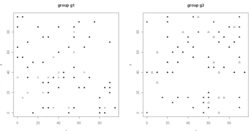
For the reasons mentioned above, we constructed an artificial set of 130 ran-domly allocated elements in a common spatial domain. The elements were not spatially segregated and were randomly assigned to one of two groups, each con-taining 65 sites. For each group, 50 sites were used for estimation, and 15 were used as a test set. Figure 1 shows the locations of the data set elements. For illus-trative purposes, they are separated into two panels that refer to the same area. Different symbols are used for the estimation and assessment sites.
Figure 1 – Maps of the simulated points belonging to the two groups in the same spatial domain (the black points were used for estimation, and the empty points were used for evaluation).
We focused on the model described in Section 4.1, which is the starting point for dealing with structural differences between elements from the same population in
a common territory. To this end, the simulation assumed identical spatial covari-ance structures (exponential ones, in this case) and specialized in different charac-terizations of the mean value, as shown in Table 1.
TABLE 1
The parameter values in the simulation study
group 1 group 2
mean 0.00 0.51
covariogram exponential C h( )2exp(- )h 2
0.23
0.08
The models that were used in this simulation followed the common hierarchi-cal structure that was illustrated in the previous sections, with a particular empha-sis on the spatial dimension.
The large-scale component can be introduced into the model by (8) or through other formulations. When the differences in the levels are specified, expression (13) is used and the consequent improvement in prediction has to be assessed.
The starting point for the comparisons is a reductive consideration of two group-specific models that are estimated separately for each data set, as shown in Figure 1. The entire data set is used for the estimates under the two different mo-dels for the large-scale components expressed by (8) and (13).
TABLE 2
Parameter syntheses: MCMC posterior means (standard errors within brackets) Parameter
values (group 1) Model 1 (group 2) Model 2 Model 3, with mean from (8) Model 4, with mean from (13)
0.05 (0.23) 0.57 (0.25) 0.27 (0.18) 0.04 (0.20) 0.51 (0.08) 2 0.43 (1.25) 0.44 (0.75) 0.27 (0.22) 0.29 (0.26) 0.08 (0.04) 0.07 (0.04) 0.09 (0.06) 0.07 (0.03) DIC 47.86 46.35 108.79 66.14
Table 2 is evaluated with respect to the population values that generated the data in Table 1 and the values assumed by the Deviance Information Criterion (DIC) (Spiegelhalter et al., 2002). These criteria are suitable for assessing the con-sequences of using models based on the entire available data set, as in the last two columns, versus models based on subsets. The index is sensitive to the number of cases, and the value obtained using the mean from (13) applied to all data actually competes with the results of the two group-specific models. The improvement from introducing separate means rather than an overall mean is dramatic. As ex-pected, the model with the mean from (8) that is summarized in the third column is not able to capture the group-specific means and estimates an unrealistic mean value. The introduction of the coefficient in (13) is reflected in the last
col-umn, where the sum of the estimated and reproduces the group 2 mean (see Table 1). The estimated posterior covariogram variances of the models for the entire data set are sensibily lower than the group-specific ones.
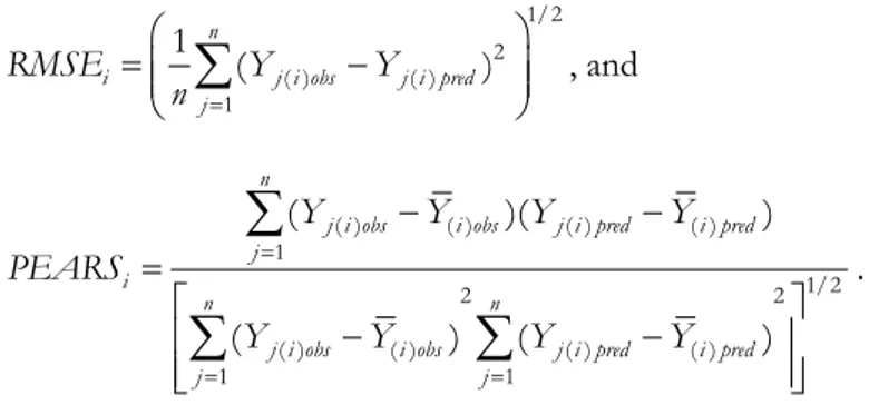
The assessment can be performed using complementary measures (see, for ex-ample, Cameletti et al., 2010). Here we consider two indices that are defined for the i-th outcome of the simulation, the RMSE (Root Mean Squared Error) and the Pearson correlation coefficient, as measures over the test set of size n:
1/2 2 ( ) ( ) 1 1 n ( ) i j i obs j i pred j RMSE Y Y n
, and ( ) ( ) ( ) ( ) 1 1/2 2 2 ( ) ( ) ( ) ( ) 1 1 ( )( ) ( ) ( ) nj i obs i obs j i pred i pred
j i
n n
j i obs i obs j i pred i pred
j j Y Y Y Y PEARS Y Y Y Y
.The results are reported in Figure 2, with a panel of boxplots for each index. The spread of the boxplots is different due to the test-set size. Models 1 and 2 of Table 2 are estimated separately for the two groups (i.e., on 50 points each) while Models 3 and 4 are estimated on the entire training set (100 points). The predic-tions involving a double-sized data set (Models 3 and 4) are analogously per-formed. Both panels indicate that Model 4 gives the best results because it has the lowest RMSE values and the highest the Pearson correlation coefficient values.
Mod1 Mod2 Mod3 Mod4
0. 2 0. 4 0. 6 RMSE
Mod1 Mod2 Mod3 Mod4
-0 .4 0. 0 0. 4 0. 8 Pearson
Figure 2 – A boxplot of the assessment indices computed for each model.
6. CONCLUDING REMARKS
The results of simulations confirm that in an overall model, expressing a large-scale component that considers groups by summarizing differences in the
inter-cept is the appropriate method for dealing with data that are characterized by dif-ferent levels and that share a common spatial structure. A hierarchical Bayesian Gaussian model with a process mean modeled by (13) is therefore the starting point for advancing in modeling differences in the large-scale component. A fur-ther extension of the mean is proposed in (14), in which differences are furfur-ther modeled by means of covariates. Differences in the spatio-temporal covariance structure can also be introduced using (16), in which the independence assump-tions between the groups are relaxed. The combination of submodels for the mean, as in (13) and (14), and for the variance-covariance structure, as in (16), is flexible and potentially includes a wide variety of models for spatio-temporal data that have been previously categorized.
Department of Statistics DANIELA COCCHI
University of Bologna FRANCESCA BRUNO
ACKNOWLEDGEMENTS
The research work underlying this paper was funded by a 2008 grant (project no. 2008CEFF37_001, sector: Economics and Statistics) for research projects of national in-terest that was provided by the Italian Ministry of Universities and Scientific and Techno-logical Research. We thank Fedele Greco, Rosalba Ignaccolo, Giovanna Jona Lasinio and Lucia Paci for the useful discussions and the continuous support.
REFERENCES
G. ADELFIO, M. CHIODI, (2009), Second-order diagnostics for space-time point processes with application to seismic events, “Environmetrics” 20, pp. 895-911.
S. BANERJEE, B.P. CARLIN, A.E. GELFAND, (2004), Hierarchical Modeling and Analysis for Spatial Data, Chapman and Hall, CRC Press.
L. BERNARDINELLI, D. CLAYTON, C. PASCUTTO, C. MONTOMOLI, M. GHISLANDI, M. SONGINI, (1995), Bayes-ian analysis of space-time variation in disease risk, “Statistics in Medicine” 14, pp. 2433-2443. D. BOHNING, (2003), Empirical Bayes estimators and non-parametric mixture models for space and
time-space disease mapping and surveillance, “Environmetrics” 14, pp. 431-451.
P.E. BROWN, K.F. KARESEN, G.O. ROBERTS, S. TONELLATO, (2000), Blur-generated non-separable space-time models, “Journal of the Royal Statistical Society” Ser. B, 62, pp. 847-860.
F. BRUNO, D. COCCHI,(2006), Seasonal spatio-temporal non-separability: the case of Ozone in Emilia Romagna, in B. Cafarelli, G. Jona Lasinio, A. Pollice (a cura di) SPATIAL-Spatial Data
Methods for Environmental and Ecological Processes, Book of Abstracts, ISBN: 88-8459-078-7, WIP Edizioni.
M. CAMELETTI, R. IGNACCOLO, S. BANDE,(2010),Comparing air-quality statistical models,GRASPA
Working paper40.
G. CHRISTAKOS,(2000), Modern spatiotemporal geostatistics, Oxford University Press, Oxford. D. COCCHI, F. GRECO, C. TRIVISANO, (2006), Displaced calibration of PM10 measurements using
spa-tio-temporal models, “STATISTICA” 66, pp. 127-138.
D. COCCHI, F. GRECO, C. TRIVISANO, (2007), Hierarchical space-time modelling of PM10 pollution,
N. CRESSIE,(1993), Statistics for Spatial Data. John Wiley & Sons, London.
N. CRESSIE,(1998), Aggregation and interaction issues in statistical modelling of spatiotemporal proc-esses, “Geoderma” 85, 133-140.
N. CRESSIE, H.C. HUANG, (1999), Classes of nonseparable, spatiotemporal stationary covariance func-tions, “Journal of the American Statistical Association” 94, pp. 1330-1340.
R. M. CRUJEIRAS, R. FERNANDEZ-CASAL, W. GONZALEZ-MANTEIGA, (2010), Nonparametric test for separability of spatio-temporal processes, “Environmetrics” 21, pp. 382-399.
L. DE CESARE, D. MYERS, D. POSA, (2001), Product-sum covariance for spacetime modeling: an
environ-mental application, “Environmetrics” 12, pp. 11-23.
P.J. DIGGLE, (1983), Statistical Analysis of Spatial Point Patterns, Academic Press, London. R. FERNANDEZ-CASAL, W. GONZALEZ-MANTEIGA, M. FEBRERO-BANDE, (2003), Flexible
spatio-temporal stationary variogram models, “Statistics and Computing” 13, pp. 127-136.
B.F. FINKENSTÄDT, L. HELD, V. ISHAM, (2007), Statistical Methods for Spatio-temporal systems, CRC
Press, Chapman and Hall.
A.S FOTHERINGHAM, M. CHARLTON, C. BRUNSDON, (1998), Geographically weighted regression: a natu-ral evolution of the expansion method for spatial data analysis, “Environment and Planning”
30, pp. 1905-1927.
M. FUENTES, (2006), Testing for separability of spatial-temporal covariance functions, “Journal of
Sta-tistical Planning and Inference” 136, pp. 447-466.
C. GAETAN, X. GUYON,(2010), Spatial Statistics and Modeling, Springer, New York.
A. GELMAN, J.B. CARLIN, H.S. STERN, D.B. RUBIN,(2004),Bayesian Data Analysis, Second Edition,
CRC Press, Chapman and Hall.
T. GNEITING,(2002), Stationary covariance functions for spacetime data, “Journal of the American
Statistical Association” 97, pp. 590-600.
T. GNEITING, M.G. GENTON, P. GUTTORP, (2007), Geostatistical space-time models, stationarity, sepa-rability and full symmetry, in B.F. FINKENSTÄDT, L. HELD, V. ISHAM, (2006), Statistical Methods
for Spatio-temporal systems, CRC Press, Chapman and Hall, pp. 151-175.
F. GRECO, C. TRIVISANO, (2009), A multivariate CAR model for improving the estimation of relative risks, “Statistics in Medicine” 28, pp. 1707-1724.
G. JONA LASINIO, A. ORASI, F. DIVINO, P.L. CONTI,(2007), Statistical contributions to the analysis of environmental risks along the coastline. In Società Italiana di Statistica - rischio e previsione.
Venezia, 6-8 giugno,cleup, pp. 255-262.
R.H. JONES, Y. ZHANG, (1997), Models for continuous stationary spacetime processes, in T.G.
Gre-goire, D.R. Brillinger, P.J. Diggle, E. Russek-Cohen, W.G. Warren, R.D. Wolfinger (eds) “Modelling longitudinal and spatially correlated data. Lecture Notes in Statistics” 122, Springer, Berlin Heidelberg New York, pp. 289-298.
M. JUN, M. L STEIN, (2004), Statistical comparison of observed and CMAQ modeled daily sulfate levels,
“Atmospheric Environment” 38, pp. 4427-4436.
A. KOLOVOS, G. CHRISTAKOS, D.T. HRISTOPULOS, M.L. SERRE, (2004), Methods for generating non-separable spatiotemporal covariance models with potential environmental applications, “Advances in
Water Resources” 27, pp. 815-830.
P.C. KYRIAKIDIS, A.G. JOURNEL, (1999), Geostatistical Space-Time Models: A Review,
“Mathemati-cal Geology” 31, pp. 651-684.
D. LEE, G. SHADDICK,(2007), Time-varying coefficient models for the analysis of air pollution and health outcome data, “Biometrics” 63, pp. 1253-1261.
B. LI, M.G. GENTON, M. SHERMAN,(2007), A nonparametric assessment of properties of space-time co-variance functions, “Journal of the American Statistical Association” 102, pp. 736-744. N. LU, D.L. ZIMMERMAN, (2005), The likelihood ratio test for a separable covariance matrix, “Statistics
C. MA,(2002), Spatio-temporal covariance functions generated by mixtures, “Mathematical Geology”
34, pp. 965-974.
M. MITCHELL, M.G. GENTON, M. GUMPERTZ, (2006), A likelihood ratio test for separability of covari-ances, “Journal of Multivariate Analysis” 97, pp. 1025-1043.
L. PACI,(2010), Hierarchical Bayesian space-time model: the case of Ozone in Emilia Romagna,
The-sis of master in statistics (in Italian).
A. POLLICE, G. JONA LASINIO,(2009), Two approaches to imputation and adjustment of air quality data from a composite monitoring network, “Journal of Data Science” 7, pp. 43-59.
A. POLLICE, G. JONA LASINIO,(2010), Spatiotemporal analysis of the PM10 concentration over the Tar-anto area, “Environmental Monitoring and Assessment” 162 (1-4), pp. 177-190. E. PORCU, P. GREGORI, J. MATEU,(2006), Nonseparable stationary anisotropic spacetime covariance
func-tions, “Stochastic Environmental Research and Risk Assessment” 21, pp. 113-122. H. SANG, A.E. GELFAND,(2009), Hierarchical modeling for extreme values observed over space and time,
“Environmental and Ecological Statistics” 16, pp. 407-426.
S.K. SAHU, A.E. GELFAND, D.M. HOLLAND,(2007), High Resolution Space-Time Ozone Modeling for Assessing Trends, “Journal of the American Statistical Association” 102, pp. 1221-1234. S.K SAHU, O. NICOLIS,(2009), An evaluation of European air pollution regulations for particulate
mat-ter monitored from a hemat-terogeneous network, “Environmetrics” 20, pp. 943-961.
D.J. SPIEGELHALTER, N.G, BEST, B.P, CARLIN, A. VAN DER LINDE,(2002),Bayesian Measures of Model Complexity and Fit (with Discussion), “Journal of the Royal Statistical Society, Series B” 64,
pp. 583-616.
M.L. STEIN,(2005), Spacetime covariance functions, “Journal of the American Statistical
Associa-tion” 100, pp. 310-321.
J. WANG, G. CHRISTAKOS, M-G. HU,(2009),Modeling spatial means of surfaces with stratified nonhom-geneity, “IEEE Transactions on Geoscience and Remote Sensing” 47, 4167-4174. C.K. WIKLE, (2003), Hierarchical models in environmental science, “International Statistical
Re-view” 71, pp. 181-199.
C.K WIKLE, L.M. BERLINER, N. CRESSIE,(1998), Hierarchical Bayesian space-time models,
“Environ-mental and Ecological Statistics” 5, pp. 117-154.
A.M. ZASLAVSKY,(2003), Hierarchical Bayesian modeling, in S.J.PRESS, Subjective and objective Bayesian statistics: principles, models and application, New York, John Wiley and Sons, pp. 336-358.
H. ZHANG,(2004),Inconsistent Estimation and Asymptotically Equal Interpolations in Model-Based Geostatistics,“Journal of the American Statistical Association”99,pp.250-261.
SUMMARY
Considering groups in the statistical modeling of spatio-temporal data
Spatio-temporal statistical methods are developing into an important research topic that goes beyond the study of processes that generate independent, identically distributed observations. Hierarchical models are a suitable proposal for both continuous and dis-crete spatio-temporal domains. They are flexible and permit separation of the various sources of uncertainty by means of a sequence of conditional models. In this work, we expanded on spatio-temporal data modeling by considering data categorization with re-spect to certain differentiating features. We studied the impact of the presence of sub-groups on model building, with emphasis on Bayesian modeling. We discussed how dif-ferences in spatial locations can be reflected in a hierarchical model and assessed the per-formances of different models via a simulation study.