A PRODUCT AUTOREGRESSIVE MODEL
WITH LOG-LAPLACE MARGINAL DISTRIBUTION K.K. Jose, M.M. Thomas
1. INTRODUCTION
In statistical distribution theory, the ‘log-Laplace distribution’ is the probability distribution of a random variable whose logarithm follows a Laplace distribution. The log-Laplace models appeared in the statistical, economic as well as science literature over the past seventy years. The relationship between Laplace distribu-tion and log-Laplace distribudistribu-tion is analogous to the reladistribu-tionship between the Normal and lognormal distributions. Most often they appeared as models for data sets with particular properties or were derived as the most natural models based on the properties of the studied processes. Thus Kozubowski and Podgór-ski (2003) review many uses of the log-Laplace distribution. Fréchet (1939) pre-sented the symmetric log-Laplace law as a model for income when the ‘moral for-tune’, that is the logarithm of income, was assumed to have the classical Laplace distribution. The asymmetric log-Laplace distribution has been a good fit to pharmacokinetic and particle size data. Particle size studies often show the log size to follow a tent-shaped distribution like the Laplace, see Julià and Veves-Rego (2005) for more details. It has been used to model growth rates, stock prices, annual gross domestic production, interest and forex rates. Some explana-tion for the goodness of fit of the Log-Laplace has been suggested because of its relationship to Brownian motion stopped at a random exponential time.
Symmetric and asymmetric forms of log-Laplace distribution were used for modeling various phenomena by a number of researchers. Inoue (1978) derived the symmetric log-Laplace distribution from his stochastic model for income dis-tribution, fitted it to income data by maximum likelihood and reported a better fit than that of a lognormal model traditionally used in this area. Uppuluri (1981) ob-tained an axiomatic characterization of this distribution and derived the distribu-tion from a set of properties about the dose-response curve for radiadistribu-tion carcino-genesis. Barndorff-Nielsen (1977) and Bagnold and Barndorff-Nielsen (1980) proposed the log-hyperbolic models, of which log-Laplace is a limiting case for particle size data. Log-Laplace models have been recently proposed for growth rates of diverse processes such as annual gross domestic product, stock prices,
interest or foreign currency exchange rates, company sizes, and other processes. Log-Laplace distributions are mixtures of lognormal distributions and have as-ymptotically linear tails. These two features makes them particularly suitable for modeling size data.
The autoregressive models associated with the exponential, gamma and mixed exponential distributions are introduced by Lawrance (1978). Gaver and Lewis (1980) also discussed these models and their properties. In the case of gamma AR(1) processes, Lawrance (1982) had shown that the innovation distribution can be generated easily as a compound Poisson distribution; it is noted that the result holds for both integral and fractional index of the gamma distribution. Dewald and Lewis (1985) introduced a first order autoregressive Laplace process. Dam-sleth and El-Shaaravi (1989) developed a time series model with Laplace noise as an alternative to the normal distribution. Gibson (1986) used an AR(1) process for image source modeling in data compression tasks. Sim (1994) discussed a general theory of model-building approach that consists of model identification, estimation, diagnostic checking and forecasting for a model with a given marginal distribution. Cox (1981) gives a wide ranging discussion of many developments in non-Gaussian, non-linear and non-reversible aspects of time series models. Seethalekshmi and Jose (2004; 2006) introduced various autoregressive models utilizing -Laplace and Pakes distributions. Jose et al. (2008) introduced a new concept of autoregressive processes which gives a combination of Gaussian and non-Gaussian time series models. Punathumparambathu (2011) introduced a new family of skewed distributions generated by the normal kernel and discussed its various applications. Jose and Krishna (2011) introduced autoregressive models having Marshall-Olkin assymmetric Laplace marginals. Jose and Abraham (2011) extend the count models with Mittag-Leffler waiting times. McKenzie (1982) de-rived a non-linear stationary stochastic process, called product autoregression structure.
Klebanov et al. (1984) introduced geometric infinite divisibility (g.i.d.) and ob-tained several characterizations in terms of characteristic functions. The class of g.i.d. distributions form a subclass of infinitely divisible (i.d.) distributions and contain the class of distributions with complete monotone derivative (c.m.d.). They also introduced and characterized the related concept of geometric strict stability (g.s.s.) for real valued random variables. The exponential and geometric distributions are examples of distributions that possess the g.i.d. and the g.s.s. properties. Mittag-Leffler distributions, Laplace distributions etc are g.i.d., see Pil-lai (1990), PilPil-lai and Sandhya (1990), Jayakumar (1997). Fujitha (1993) constructed a larger class of g.i.d. distributions with support on the non-negative half-line. Bondesson (1979) and Shanbhag and Sreehari (1977) have established the self-decomposability of many of the most commonly occurring distributions in prac-tice. Bondesson (1981) noted that the stationary marginal distribution of an AR(1) process belongs to class L, otherwise called the class of self-decomposable distributions. Kozubowski and Podgórski (2010) introduced a notion of random decomposability and discussed its relation to the concepts of self-decomposability and g.i.d..
In this paper we consider log-Laplace distributions and their multivariate ex-tensions along with applications in time series modeling using product autore-gression. Section 1 is introductory. In section 2, the log-Laplace distribution and its properties are studied. Various divisibility properties like infinite divisibility and geometric infinite divisibility are studied. Multiplicative infinite divisibility and geometric multiplicative infinite divisibility are introduced and studied. In section 3, product autoregression models are introduced and studied. Section 4 deals with additive autoregressive model. The generation of the process, sample path prop-erties and estimation of parameters are considered here. In section 5, a more gen-eral model with double Pareto lognormal marginals is introduced. Multivariate extension is given in section 6.
2. THE LOG-LAPLACE DISTRIBUTION AND ITS PROPERTIES
A random variable Y is said to have a log-Laplace distribution with parame-ters > 0, > 0 and > 0 (LL( , , )) if its probability density function is
1 1 for 0 < < 1 ( ) = . for y y g y y y (1)
The cumulative density function has the form
0 for 0 ( ) = for 0 < . 1 for y y G y y y y (2)
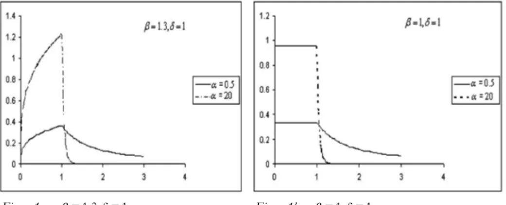
This distribution can be derived by combining the two power laws and has power tails at zero and at infinity. This density has a distinct ‘tent’ shape when plotted on the log scale. The graphs of probability density function of log-Laplace distribution for fixed and for various values of are given in the fol-lowing figures.
Figure 1a – = 1.3, = 1 . Figure 1b – = 1, = 1 .
The log-Laplace pdf (1) can be derived as the distribution of eX where X is
an asymmetric Laplace (AL) variable with density exp( ( )) for < ( ) = exp( ( )) for x x f x x x (3)
Therefore if X has an AL distribution given by (3), then the density of = eY X
is given by (1) with = e .
Kozubowski and Podgórski (2003) studied some important properties of LL( , , ). It has Pareto-type tails at zero and infinity, that is
1 ( > ) ~ as and P Y x C x x 2 (0 < ) ~ as 0 . P Y x C x x
It also possesses invariance property with respect to scaling and exponentiation which is natural property of variables describing multiplicative processes such as growth. The distribution has a representation as an exponential growth-decay process over random exponential time which extends a similar property of the Pareto distribution by allowing decay in addition to growth. Its simplicity allows for efficient practical applications and thus gives an advantage over many other models for heavy power tails, such as stable or geometric stable laws. The upper tail index is not bounded from above which adds flexibility over some other models for heavy tail data such as stable or geometric stable laws where its value is limited by two. Maximum entropy property of LL distribution is desirable in many applications. Stability with respect to geometric multiplication which may play a fundamental role in modeling growth rates. Limiting distribution of geo-metric products of LL random variables leads to useful approximations. Its straightforward extension to the multivariate setting allows modeling of corre-lated multivariate rate data, such as joint returns on portfolios of securities.
Let =Y d LL( , , ), and let c> 0,r , then 0 cY LL=d (c , , ), LL( , / , / ) for > 0 = . LL( , /| |, /| |) for < 0 r d r r r r r Y r r r In particular, if =Y LLd ( , , ) then 1=d
Y LL(1/ , , ), and we have the
recip-rocal property 1=dY
Y , if = and also = 1 .
The characteristic function of the LL(1, , ) random variable Y has the form
E(e ) =itY M( , 1, )it t C t[ ( , ) iS t( , )], where
(4) =1 ( ) ( , , ) = 1 , for > 0, > 0, ( ) ! n n n n a z M a b z a b z b n
C, ( ) = (a n a a1) ( a n 1) is the confluent hypergeometric function and ( , ) = a 1cos dx
C x a
t t t and1
( , ) = a sin d
x
S x a
t t t are the generalized Fresnel integrals. For details on Fresnel integralsand their properties see Abramowitz and Stegan (1964).LL distributions are heavy tailed and some moments do not exist.The mean and the variance are finite only if > 1 and > 2 respectively. Due to reciprocal properties of these laws, the harmonic mean is of the same form as the reciprocal of the mean. We also note that LL distributions are unimodal with the mode at
when > 1 and the mode at zero when < 1.
Mean = , > 1 ( 1)( 1) moment = , < < ( )( ) th r r r r r 2 2 Variance = , > 2 ( 2)( 2) ( 1)( 1)
Log-Laplace distributions can be represented in terms of other well-known dis-tributions, including the lognormal, exponential, uniform, Pareto, and beta distri-butions. The log-Laplace distribution LL( , , ) can be viewed as a lognormal
distribution LN( , ), where the parameters and are random. This is a di-rect consequence of the fact that an asymmetric Laplace random variable can be viewed as a normal variable with the above random mean and standard devia-tion (see Kotz et al. (2001)). More specifically, the variable ~Y LL( , , ) has the representation
=ed ,
Y R
where R is standard lognormal random variable,
1 1 = log E and 2 = E,
where E is a standard exponential variable independent of R .
As a direct consequence of the fact that a skew Laplace variable arises as a dif-ference of two independent exponential variables, we have
1 1 1 2
= ed E E ,
Y
where E and 1 E are two independently and identically distributed (i.i.d.) stan-2
dard exponential variables. Let U and 1 U be independent random variables dis-2
tributed uniformly on [0, 1]. Then we have
1/ 1 1/ 2 =d U . Y U
LL random variable can also be represented as the ratio of two Pareto random variables of the form
1 2 =d P , Y P
where P and 1 P are independent Pareto random variables with parameters 2
and respectively, for more details, see Kozubowski and Podgórski (2003). Entropy, basic concept in information theory is a measure of uncertainty asso-ciated with the distribution of a random variable Y and is defined as
H( ) = E[ log ( )].Y f Y
It has found applications in a variety of fields, including statistical mechanics, queuing theory, stock market analysis, image analysis and reliability. If
~
1 1 1 1 H( ) = 1 logY log .
For an AL random variable X , entropy is given by
1 1 H( ) = logX .
The entropy is maximized for an AL distribution and hence the same property holds for LL distribution also, see Kozubowski and Podgórski (2003). Jose and Naik (2008) introduced asymmetric pathway distributions and showed that the model maximizes various entropies.
The estimation of parameters of the log-Laplace distribution is given by Hinkley and Revankar (1977). They give Fisher information matrix of the LL random variable. The maximum likelihood estimates of the parameters are given by Hartley and Revankar (1974). They showed that these estimators are asymp-totically normal and efficient.
2.1. Multivariate Extension
Let X= (X1, , X d) follows a multivariate asymmetric Laplace distribution with characteristic function
1 1 ( ) = 1 ' ' 2 t i t t m t (5)
where 't denotes transpose of ,t mRd and is a d d non-negative definite
symmetric matrix. A d-dimensional log-Laplace variable can be defined as a ran-dom vector of the form
1
= e = (e , ,eX X Xd ) .
Y
If is positive-definite, then the distribution is d-dimensional and the corre-sponding density function can be derived easily from that of the Laplace distribu-tion, see Kotz et al. (2001), as
1 1 =1 ( ) = (log ) d i , = ( , , d) > 0, i g f y y y y y
Y
/2 1 ' 1 1 1 /2 1/2 1 2 ' ( ) = (2 ' )( ' ) , 0 (2 ) | | 2 ' x m d e x x f x K m m x x x m m Σ Σ Σ Σ Σ Σis the density of multivariate asymmetric Laplace distribution. Here = 1 d/2 and K is the modified Bessel function of the third kind.
Similar to the univariate case, multivariate LL distribution also possesses the stability and limiting properties with respect to geometric multiplication. Each component of a multivariate LL random vector is univariate LL.
2.2. Divisibility properties
The notions of infinite divisibility (i.d.) and geometric infinite divisibility (g.i.d.) play a fundamental role in the study of central limit theorem and Lévy processes. Variables appearing in many applications in various sciences can often be repre-sented as sums of larger number of tiny variables, often independently and identi-cally distributed. The theory of infinite divisible distributions was developed pri-marily during the period from 1920 to 1950.
Definition 2.1. A probability distribution with characteristic function is i.d. if for any integer n 1, we have
=[ ] ,n n
where n is another characteristic function. In other words, a random variable
X with characteristic function has the representation
=1
=d n i,
i
X
Xfor some i.i.d. random variables X . i Remark 2.1. AL distributions are i.d.. Remark 2.2. LL distributions are not i.d..
Definition 2.2. A random variable X and its probability distribution is said to be
g.i.d. if for any p (0,1) it satisfies the relation
( ) =1 =d p i , p i X X
( )i p
X are i.i.d. for each p , and p and (X( )pi ) are independently distributed, see
Klebanov et al. (1984).
Characterization of g.i.d.. A random variable X is g.i.d. if and only if (iff)
1 ( ) = , 1 ( ) X t t
where ( ) t is a non-negative function with complete monotone derivative (c.m.d.) and (0) = 0 .
Now we consider the divisibility properties with respect to multiplication. Ko-zubowski and Podgórski (2003) discussed the multiplicative divisibility and multi-plicative geometric divisibility. There is no further developments on this area in the literature.
Definition 2.3. A random variable Y is said to be multiplicative infinitely divisible
(m.i.d.) if it has the representation
=1
=d n i, = 1, 2,3, ,
i
Y
Y n for some i.i.d. random variables Y . i Theorem 2.1. LL distributions are m.i.d..
Proof. Let Y follows the LL distribution. We have to prove that
=1
=d n i,
i
Y
Ywhere Y ’s are i.i.d. random variables. i
Taking logarithm on both sides we get log =Y
ni=1logYi. Since we know that = logX Y AL distributions, we need only to prove that X is i.d.. ALdis-tributions are i.d.. Therefore it follows that LL disdis-tributions are m.i.d..
Definition 2.4. A random variable Y is said to be geometric multiplicative
infi-nitely divisible (g.m.i.d.) if for any p (0,1), it satisfies the relation
( ) =1 = , p d i p i Y Y
where p is a geometric random variable with mean 1/p , the random variables ( )i
p
Y are i.i.d. for each p , and p and (Yp( )i ) are independently distributed.
Characterization of g.i.d.. A random variable X is g.m.i.d. iff log 1 ( ) = , 1 ( ) X t t
where ( ) t is a non-negative function with complete monotone derivative (c.m.d.) and (0) = 0 .
Theorem 2.2. LL distributions are g.m.i.d..
The proof follows from the fact that log-Laplace laws arise as limits of the products of the form 1 2
p
Y Y Y of i.i.d. random variables with geometric num-ber of terms, since Laplace distributions are limits of sums of random variables
1 2 p
X X X with a geometric number of terms.
3. PRODUCT AUTOREGRESSION
McKenzie (1982) introduced a product autoregression structure. A product autoregression structure of order one (PAR(1)) has the form
1
= a , 0 < 1, = 0, 1, 2, ,
n n n
Y Y a n (6)
where { }n is a sequence of i.i.d. positive random variables. In the usual
non-linear autoregressive models, we have an additive noise. But in product autore-gressive models, we have a non-additive but multiplicative noise. We may deter-mine the correlation structure as follows.
1 = a n n n Y Y 1 =0 = k n iai n kak i Y
Assuming stationarity, 1 =0 E( ) = k E( ai ) E( ak ) n n k n k i Y Y Y
1 1 1 =0 E( ) E( ) = E( ) E( ) i a k k a n n k ai i Y Y Y Y Y
1 E( )E( ) = E( ) k a k a Y Y Y (7) Now consider the autocorrelation function Y( ) = Corr( ,k Y Yn n k ), when Yhas a log-Laplace distribution.
( 2)( 2) ( ) = ( 1)( 1) Y k k k ( )( )( 2 1)( 2 1) ( 1)( 1) , > 2 ( 1) ( 1) ( 2)( 2) k k k k (8)
The usual additive first order autoregressive model is given by
1
= , 0 < < 1, = 0, 1, 2, ,
n n n
X aX a n (9)
where { }n is the innovation sequence of i.i.d. random variables. Its
autocorrela-tion funcautocorrela-tion is given by ( ) = k, = 0, 1, 2,
X k a k
. From (8), it is clear that the correlation structure is not preserved in the case of log-Laplace process. It is well known that the correlation structure is not preserved in going from the log-normal to the log-normal distributions. McKenzie (1982) showed that the gamma distribution is the only one for which the PAR(1) process has the Markov correla-tion structure.
3.1. Self-decomposability
Definition 3.1. (Maejima and Naito, 1998) A characteristic function is semi-self-decomposable if for some 0 < < 1a , there exists a characteristic function a
such that ( ) = ( ) ( ), t at a t tR. If this relation holds for every 0 < < 1a , then is self-decomposable (s.d.) or the corresponding distribution is said to belong to L-class.
The basic problem in time series analysis is to find the distribution of { }n .
The class of s.d. distributions form a subset of the class of infinitely divisible dis-tributions and they include the stable disdis-tributions as proper subset. A number of authors have examined the L-class in detail and many of its members are now well known.
Definition 3.2.(Kozubowski and Podgórski (2010)) A distribution with
characteris-tic function is randomly self-decomposable (r.s.d.) if for each ,p c [0,1] there exists a probability distribution with characteristic function c p, satisfying
,
( ) =t c p( )[t p (1 p) ( )]ct
.
Definition 3.3. A characteristic function is multiplicative self-decomposable (m.s.d.) if for every 0 < < 1a , there exists a characteristic function loga such that
logX( ) =t logX( )at loga( ),t t
R.
The distributions in the L-class are several which are the distributions of the natural logarithms of random variables whose distributions are also self-decomposable. These include the normal, the log gamma and the log F distribu-tions. This phenomenon is very interesting in a time series point of view because the logarithmic transformation is the commonest of all transformations used in time series analysis.
4. AUTOREGRESSIVE MODEL
If we take logarithms of Y in (6), and let n Xn= logY , then the stationary n
process of {X has the form n}
1
= , where = log ,
n n n n n
X aX (10)
which has the form of linear additive autoregressive model of order one. Then we can proceed as in the case of AR(1) processes. Now from (10), under the assump-tion of staassump-tionarity, we can obtain the characteristic funcassump-tion of as
( ) ( ) = . ( ) X X t t at (11)
We know that X follows an asymmetric Laplace distribution with characteris-tic function, 2 2 e ( ) = 1 , < < , > 0, < < . (1 ) 2 i t t t t i t
This characteristic function can be factored as
1 1 ( ) = e , 1 1 2 2 i t t i t i t (12)
where > 0, = 1 2
, see Kotz et al. (2001). Then substituting (12) in (11), we get
(1 ) (1 ) e 2 2 ( ) = e (1 ) (1 ) 2 2 i t i at i at i at t i t i t = e (1 ) (1 ) 1 (1 ) 1 . (1 ) (1 ) 2 2 i a t a a a a i t i t (13)
This implies that has a convolution structure of the form,
1 2
=dU V V ,
(14)
where U is a degenerate random variable taking value (1 with probability a) one and V and 1 V are convolutions of 2 T and 1 T where, 2
1 1 0, with probability = , with probability 1 a T E a 2 2 0, with probability = , with probability 1 a T E a
where E and 1 E are exponential random variables with means 2
2 and 2 respectively. 4.2. Sample path properties
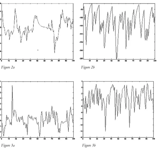
Sample path properties of the process are studied by generating 100 observa-tions each from the process with various parameter ( , , ) combinations. In Figures 4a and 4b, we take = 0.7a and the values of ( , , ) as (0, 1, 1) and (0, 10, 10) respectively. In Figures 5a and 5b, we take = 0.4a and the values of
, ,
( ) as (0, 1, 1) and (0, 2, 2) respectively. The process exhibits both positive and negative values with upward as well as downward runs as seen from the fig-ures.
Figure 2a Figure 2b
Figure 3a Figure 3b
4.3. Estimation of parameters
The moments and cumulants of the sequence of innovations { }n can be
ob-tained directly from (13) as
2 2 2 2 1 1 E( ) = (1 ) , Var( ) = (1 ) 2 2 n a n a 1 ( 1)!(1 ) if > 1 is odd 2 and = . 1 ( 1)!(1 ) if is even 2 n n n n n n n n n n a n k n a n
Since the mean and variance of AL distribution are
2 2 2 1 1 E( ) = and Var( ) = 2 2 X X
and the higher order cumulants are given by 1 ( 1)! if > 1 is odd 2 = . 1 ( 1)! if is even 2 n n n n n n n n n k n n
From the cumulants the higher order moments can be obtained easily since
2 3= 3, 4= 4 3 2
k k and k5=510 2 3. Hence the problem of estimation
of parameters of the process can be tackled in a way similar to the method of moments.
Remark 4.1. Another more general model can be constructed by considering the
double Pareto lognormal distribution of Reed and Jorgensen (2004). 5. DOUBLE PARETO LOGNORMAL DISTRIBUTION
The double Pareto lognormal (DPLN) distribution is an exponentiated version of Normal-Laplace random variable, which results from the convolution of inde-pendent Normal and asymmetric Laplace densities. This name was coined be-cause the distribution results from the product of independently distributed dou-ble Pareto and lognormal components. It has applications in modelling the size distributions of various phenomena arising in economics (distributions of in-comes and earnings); finance (stock price returns); geography (populations of human settlements); physical sciences (particle sizes) and geology (oil-field vol-umes), see Reed and Jorgensen (2004). Similar to the log-Laplace distributions, the DPLN distribution can be represented as a continuous mixture of lognormal distributions with different variances.
A random variable Y is said to have a DPLN distribution if its pdf is
2 2 2 1 1 2 1 1 1 1 1 2 ln ( ) = exp 2 Y y f y y 2 2 2 1 1 2 2 2 ln exp . 2 c y y
2 1 2
( , , , )
Y DPLN to denote a random variable follows double Pareto
log-normal distribution.
A DPLN 2
1 2
( , , , ) random variable can be expressed as =d ,
Y UQ
where U is lognormally distributed and Q is the ratio of the Pareto random
variables, known as double Pareto random variable. The moment generating function does not exist for a DPLN distribution. The lower order moments about zero are given by
2 2 ' 1 2 1 1 2 = E( ) = exp for < . ( )( ) 2 r r r X r r r r However ' r
does not exist for r . The mean (for 1 1> 1) is 2 1 2 2 1 2 E( ) = e ( 1)( 1) X
and the variance (for 1> 2) is 2 2 2 2 2 1 2 1 2 1 2 2 2 1 2 1 2 e ( 1) ( 1) Var( ) = e ( 2)( 2) ( 1) ( 1) X
5.1. Product Autoregression with DPLN marginals
We can develop a product autoregression model given in (6) if ~
n
Y DPLN( 1, , ,2 2). The autocorrelation function has the form, 2 1 2 1 2 1 2 1 2 2 2 2 1 2 1 2 1 2 e ( )( )( 1)( 1) ( 1)( 1) ( ) = . e ( 1) ( 1) ( 2)( 2) k a k k k k Y a a a a k (15)
Here also the correlation structure is not preserved. It is well known that the cor-relation structure is not preserved in going from the lognormal to the normal dis-tributions.
If we take logarithms of Y in (6), and let n Xn = logY , then the stationary n
DPLN( 1, 2, , 2) distribution, X= log ~Y Normal-Laplace distribution
(NL( 1, , ,2 2)) having the characteristic function given by 2 2 1 2 1 2 ( ) = exp . 2 ( )( ) X t i t t it it (16)
For further analysis, we can use the linear AR(1) model with Normal-Laplace marginals developed by Jose et al. (2008). They showed that the innovations { }n
is distributed as the convolution of the Normal and exponentially tailed densities. The Normal-Laplace model combines Gaussian and non-Gaussian marginals to model time series data. Normal-Laplace distribution has various applications in the areas of financial modeling, Lévy process, Brownian motion, see Reed (2007). 6. MULTIVARIATE PRODUCT AUTOREGRESSION
A multivariate product autoregression structure of order one (PAR(1)) has the form
1
= a , 0 < 1, = 0, 1, 2, ,
n n n a n
Y Y ε (17)
where { }Y and { }n ε are sequence of positive d -variate random vectors and n
they are independently distributed. Here also we have a non-additive noise. For further analysis, we can take logarithms of Yn in (17), and let Xn = logY . n
Then obtain a multivariate linear AR(1) model,
1
= , 0 < < 1
n a n n a
X X η (18)
where Xn and innovations ηn = logεn are d - variate random vectors. Clearly we
know that X follows a multivariate asymmetric Laplace distribution having the n
characteristic function given in (5). Then the characteristic function of ηn can be
obtained from ( ) ( ) = , ( )a X η X t t t where ( ) = E(exp ' ).i X t t X
7. CONCLUSION
The log-Laplace distribution and its important properties and its extension to multivariate case are studied. Some divisibility properties like infinite divisibility, geometric infinite disability and divisibility properties with respect to multiplica-tion, namely multiplicative infinite divisibility, geometric multiplicative infinite di-visibility properties are explored. A product autoregression structure with log-Laplace marginals is developed. Self-decomposability property is studied. A linear AR(1) model is developed along with the sample path properties and the estima-tion of parameters of the process. A more general model with double Pareto log-normal marginals is discussed. A multivariate extension of the product autore-gression structure is also considered.
ACKNOWLEDGEMENTS
The authors are grateful to the reviewer for the valuable suggestions which helped in improving the paper. The authors are also grateful to the Department of Science and Technology (DST), Govt. of India for the financial support under the INSPIRE Fellow-ship.
Department of Statistics, St. Thomas College, Palai, K.K. JOSE
Mahatma Gandhi University, Kottayam MANU MARIAM THOMAS
REFERENCES
M. ABRAMOWITZ, I.A. STEGUN (1964). Handbook of Mathematical Functions, U.S. Department of Commerce, National Bureau of Standards, Applied Mathematics Series 55.
R.A. BAGNOLD, O. BARNDORFF-NIELSEN (1980). The pattern of natural size distribution. “Sedimen-tology” 27, pp. 199-207.
O. BARNDORFF-NIELSEN (1977). Exponentially decreasing distributions for the logarithm of particle
size. ‘Proceedings of Royal Society London A” 353, pp. 401-419.
L. BONDESSON (1979). A general result on infinite-divisibility. “Annals of Probability” 7, pp. 965-979.
L. BONDESSON (1981). Discussion of the paper Cox “Statistical analysis of time series: Some recent
de-velopments”. “Scandinavian Journal of Statistics” 8, pp. 93-115.
D.R. COX (1981). Statistical Analysis of Time Series: Some Recent Developments. “Scandinavian Journal of Statistics” 8, pp. 93-115.
E. DAMSLETH, A.H. EL-SHAARAWI (1989). ARMA models with double-exponentially distributed noise. “Jornal of Royal Statistical Society B” 51(1), pp. 61-69.
L.S. DEWALD, P.A.W. LEWIS (1985). A new Laplace second-order autoregressive time-series model-
NLAR(2). “IEEE Transactions on Information Theory” IT 31(5), pp. 645-651.
M. FRÉCHET (1939). Sur les formules de répartition des revenus, “Revue l’Institut International de Statistique” 7(1), pp. 32-38.
Y. FUJITHA (1993). A generalization of the results of Pillai. “Annals of Institute of Statistical Mathematics” 45, pp. 361-365.
D.P. GAVER, P.A.W. LEWIS (1980). First order autoregressive gamma sequences and point processes. “Ad-vances in Applied Probability” 12, pp. 727-745.
J.D. GIBSON (1986). Data compression of a first order intermittently excited AR process. In Statistical Image Processing and Graphics. pp. 115-126 (Edited by E.J. Wegman and D.J. De-priest, Marcel Deckrer Inc., New York).
M.J. HARTLEY, N.S. REVANKAR (1974). On the estimation of the Pareto law from underreported data, “Journal of Econometrics” 2, pp. 327-341.
D.V. HINKLEY, N.S. REVANKAR (1977). Estimation of the Pareto law from under reported data, “Jour-nal of Econometrics” 5, pp. 1-11.
T. INOUE (1978). On Income Distribution: The Welfare Implications of the General Equilibrium
Model, and the Stochastic Processes of Income Distribution Formation, Ph.D. Thesis, University
of Minnesota.
K. JAYAKUMAR (1997). First order autoregressive semi-alpha-Laplace processes, “Statistica”, LVII, pp. 455-463.
K.K. JOSE, T. LISHAMOL, J. SREEKUMAR (2008). Autoregressive processes with normal Laplace marginals. “Statistics and Probability Letters” 78, pp. 2456-2462.
K.K. JOSE, S.R. NAIK (2008). A class of asymmetric pathway distributions and an entropy interpretation. “Physica A: Statistical Mechanics and its Applications” 387(28), pp. 6943-6951. K. K. JOSE, B. ABRAHAM (2011). A Count Model based on with Mittag-Leffler interarrival times,
“Sta-tistica”, anno LXXI, n. 4, 501-514.
O. JULIÀ, J. VIVES-REGO (2005). Skew-Laplace distribution in Gram-negative bacterial axenic cultures:
new insights into intrinsic cellular heterogeneity. “Microbiology” 151, pp. 749-755.
L.B. KLEBANOV, G.M. MANIYA, I.A. MELAMED (1984). A problem of Zolotarev and analogs of infinitely
divisible and stable distribution in a scheme for summing a random number of random variables.
“Theory of Probability and its Applications” 29, pp. 791-794.
S. KOTZ, T.J. KOZUBOWSKI, K. PODGORSKI (2001). The Laplace Distribution and Generalizations - A
Revisit with Applications to Communications, Economics, Engineering and Finance. Birkhäuser,
Boston.
T.J. KOZUBOWSKI, K. PODGORSKI (2003). Log-Laplace distributions. “International Journal of Mathematics” 3 (4), pp. 467-495.
T.J. KOZUBOWSKI, K. PODGORSKI (2010). Random self-decomposability and autoregressive processes. “Statistics and Probability Letters” 80, pp. 1606-1611.
E. KRISHNA, K. K. JOSE (2011). Marshall-Olkin assymmetric Laplace distribution and processes, “Sta-tistica”, anno LXXI, n. 4, 453-467.
A.J. LAWRANCE (1978). Some autoregressive models for point processes. “In Proceedings of Bolyai Mathematical Society Colloquiuon point processes and queuing problems” 24, Hun-gary, pp. 257-275.
A.J. LAWRANCE (1982). The innovation distribution of a gamma distributed autoregressive process. “Scandinavian Journal of Statistics” 9, pp. 234-236.
M. MAEJIMA, Y. NAITO (1998). Semi-self decomposable distributions and a new class of limit theorems. “Probability Theory and Related Fields” 112, pp. 13-31.
E.D. MCKENZIE (1982). Product autoregression: a time-series characterization of the gamma distribution. “ Journal of Applied Probability” 19, pp. 463-468.
R.N. PILLAI (1990). Harmonic mixtures and geometric infinite divisibility. “Jornal of Indian Statisti-cal Association” 28, pp. 87-98.
R.N. PILLAI, E. SANDHYA (1990). Distributions with complete monotone derivative and geometric infinite
divisibility. “Advances in Applied Probability” 22, pp. 751-754.
B. PUNATHUMPARAMBATH (2011). A new family of skewed slash distributions generated by the normal
W.J. REED (2007). Brownian Laplace motion and its use in financial modelling. “Communications in Statistics-Theory and Methods” 36, pp. 473-484.
W.J. REED, M. JORGENSEN (2004). The double Pareto lognormal distribution-a new parametric model for
size distributions. “Communications in Statistics-Theory and Methods” 33(8), pp.
1733-1753.
V. SEETHALEKSHMI, K.K. JOSE (2004). An autoregressive process with geometric
-Laplace marginals. “Statistical Papers” 45, pp. 337-350.V. SEETHALEKSHMI, K.K. JOSE (2006). Autoregressive processes with Pakes and geometric Pakes
general-ized Linnik marginals. “Statistics and Probability Letters” 76(2), 318-326.
D.N. SHANBHAG, M. SREEHARI (1977). On certain self-decomposable distributions. “Z. War-scheinlichkeitstch” 38, pp. 217-222.
C.H. SIM (1994). Modelling non-normal first order autoregressive time series. “Journal of Forecast-ing” 13, pp. 369-381.
V.R.R. UPPULURI (1981). Some properties of log-Laplace distribution. “Statistical Distributions in Scientific Work” 4, (eds., G.P. Patil, C. Taillie and B. Baldessari), Dordrecht: Reidel, 105-110.
SUMMARY
A product autoregressive model with log-Laplace marginal distribution
The log-Laplace distribution and its properties are considered. Some important proper-ties like multiplicative infinite divisibility, geometric multiplicative infinite divisibility and self-decomposability are discussed. A first order product autoregressive model with log-Laplace marginal distribution is developed. Simulation studies are conducted as well as sample path properties and estimation of parameters of the process are discussed. Further multivariate extensions are also considered.