IN PRESS: Behavioural Processes (Febr, 2018) Special issue dedicated to Ralph R. Miller
A Comparator-Hypothesis Account of Biased Contingency Detection
Miguel A. Vadillo1 & Itxaso Barberia2
1 Departamento de Psicología Básica, Universidad Autónoma de Madrid, Spain 2 Departament de Cognició, Desenvolupament i Psicologia de l’Educació, Universitat de
Barcelona, Spain
Mailing address:
Miguel A. Vadillo
Departamento de Psicología Básica Facultad de Psicología
Universidad Autónoma de Madrid 28049 Madrid, Spain
Abstract
Our ability to detect statistical dependencies between different events in the
environment is strongly biased by the number of coincidences between them. Even when there is no true covariation between a cue and an outcome, if the marginal probability of either of them is high, people tend to perceive some degree of statistical contingency between both events. The present paper explores the ability of the Comparator Hypothesis to explain the general pattern of results observed in this literature. Our simulations show that this model can account for the biasing effects of the marginal probabilities of cues and outcomes. Furthermore, the overall fit of the Comparator Hypothesis to a sample of
experimental conditions from previous studies is comparable to that of the popular
Rescorla-Wagner model. These results should encourage researchers to further explore and put to the test the predictions of the Comparator Hypothesis in the domain of biased
contingency detection.
Keywords: associative learning; Comparator Hypothesis; contingency; cue-density
Coincidences don’t matter. One could summarize with this sentence the discoveries made during the 60’s in the area of associative learning. The famous studies conducted by Kamin, Rescorla, Wagner and colleagues showed that simply pairing a conditioned stimulus (CS) and an unconditioned stimulus (US) was not enough to establish
conditioning (Kamin, 1968; Rescorla, 1968, Wagner, Logan, Haberlandt, & Price, 1968). Instead, the CS had to possess some predictive value over the US, that is, it had to provide some additional information about the probability of the US over and beyond alternative predictors. Most of the theoretical proposals published over the following decades
incorporated this principle in one way or another (Mackintosh, 1975; Rescorla & Wagner, 1972; Wagner, 1981). The only noticeable exception to this general trend is the
Comparator Hypothesis (Miller & Matzel, 1988), which assumes that learning is driven by mere contiguity (i.e., by CS-US pairings) and that sensitivity to other factors like predictive value is related to additional processes that have little to do with learning.
Interestingly, a growing body of research in human contingency learning shows quite convincingly that coincidences do matter (Griffits & Tenenbaum, 2007; Johansen &
Osman, 2015; McKenzie & Mikkelsen, 2007). Multiple experiments have shown that, other things being equal, the extent to which people perceive that a cue and an outcome are related strongly depends on the number of times they have co-occurred (e.g., Kao &
Wasserman, 1993; Levin, Wasserman, & Kao, 1993; Wasserman, Dorner, & Kao, 1990). For instance, people seem to face difficulties to detect the lack of statistical contingency between two events when their marginal probabilities are high and their coincidences are, therefore, frequent (Blanco, Matute, & Vadillo, 2013). It has been proposed that the biasing impact of these coincidences might explain why people develop causal illusions and illusory correlations (e.g., Barberia, Blanco, Cubillas, & Matute, 2013; Lilienfeld,
Ritschel, Lynn, Cautin, & Latzman, 2014; Matute et al., 2015; Matute, Yarritu, & Vadillo, 2011; Watts, Smith, & Lilienfeld, 2015).
Within the associative learning tradition, these effects have typically been explained in terms of error-correction learning algorithms like the one proposed by Rescorla and Wagner (1972; e.g., see López, Cobos, Caño, & Shanks, 1998; Shanks, 1995). As
explained in the opening paragraph, these models assume that in the long run the strength of the association between a cue and an outcome is more strongly determined by the
predictive value of the cue than by the overall number of coincidences between both events (Chapman & Robbins, 1990; Danks, 2003; Wasserman, Elek, Chatlosh, & Baker, 1993). But in the short run, before the associative strength reaches its asymptote, coincidences may have a temporary biasing effect. Consequently, these models do anticipate an effect of coincidences over predictive value, even if it is a short-lived one.
It is perhaps puzzling that the Comparator Hypothesis, the main associative model assuming that learning is driven by cue-outcome contiguity, has not been usually invoked to account for the biasing effects of coincidences on human contingency learning. The goal of the present paper is to explore the ability of this model to explain the general pattern of results observed in this literature. In the following paragraphs, we provide an overview of current research on biases in human contingency learning, including a description of conventional research methods and relevant normative analyses. Then, we present a series of simulations of the Comparator Hypothesis confirming that it can account for these biases and that its predictions deviate substantially from alternative theories. Finally, we assess the relative fit of the Comparator Hypothesis and the Rescorla-Wagner model to the results of several studies conducted by the first author and colleagues.
In a typical human contingency learning experiment, participants are asked to judge the strength of the relationship between a cue and an outcome after being exposed to a sequence of trials in which the cue can be present or absent and the outcome follows or not (e.g., Wasserman, 1990a). For instance, a popular procedure to implement these
experiments is to present participants with a cover story in which they are asked to imagine that they are physicians exploring the relationship between taking a medicine and
developing an allergic reaction. In each trial, they see the medical record of a different patient. They are told whether the patient took the medicine or not. Then, they are typically asked to predict whether that patient would develop an allergy or not. Finally, they are given feedback and they proceed to see the next patient. After seeing all the patients, they are invited to judge the relationship between taking the medicine and developing the allergic reaction, for instance on a numerical scale from -100, indicating a perfectly negative correlation between the medicine and the allergy (i.e., patients who take the medicine are less likely to develop the allergy), to +100, indicating a perfectly positive correlation.
This procedure allows researchers to present participants with four different types of trials: trials in which both the cue (medicine) and the outcome (allergy) are present (type a trials), trials in which the cue is present and the outcome is absent (type b trials), trials in which the cue is absent but the outcome is present (type c trials), and trials in which both events are absent (type d trials). By manipulating the frequencies of each type of trial (a-d) across the sequence of trials, researchers can expose participants to different cue-outcome contingencies and test how participants’ judgments change accordingly.
Although different descriptive and normative indexes of contingency have been proposed (for reviews, see Perales, Catena, Cándido, & Maldonado, 2017; Perales &
Shanks, 2007), the simplest and most popular measure of one-way contingency is the ΔP index, given by equation:
ΔP = P(o|c) - P(o|~c) (1)
where P(o|c) is the probability of the outcome given the cue and P(o|~c) is the probability of the outcome in the absence of the cue. Note that these two probabilities can be easily computed from the frequencies of each trial type, a, b, c and d. P(o|c) can be computed as a/(a+b) and P(o|~c) can be computed as c/(c+d).
In general, numerous experiments have shown that participants’ judgments of contingency are sensitive to ΔP (e.g., López et al., 1998; Shanks & Dickinson, 1987; Wasserman, 1990b; Wasserman et al., 1993). To the extent that this can be taken as a normative index of contingency (Allan, 1980; Cheng & Novick, 1992; Jenkins & Ward, 1965), this means that participants’ behavior can be considered “rational”. However, it is well known that judgments also tend to deviate from ΔP depending on factors that increase the number of coincidences between the cue and the outcome. For instance, for any fixed level of ΔP, participants’ judgments tend to increase with the overall probability of the outcome, P(o), an effect known as the outcome-density bias (e.g., Allan & Jenkins, 1983; Allan, Siegel, & Tangen, 2005; Buehner, Cheng, & Clifford, 2003; López et al., 1998; Msetfi, Murphy, Simpson, & Kornbrot, 2005; Moreno-Fernández, Blanco, & Matute, 2017; Musca, Vadillo, Blanco, & Matute, 2010; Wasserman, Kao, Van-Hamme, Katagiri, & Young, 1996). Similarly, for any fixed level of ΔP, judgments tend to increase with the overall probability of the cue, P(c), an effect known as the cue-density bias (e.g., Allan & Jenkins, 1983; Matute et al., 2011; Perales, Catena, Shanks, & González, 2005; Vadillo, Musca, Blanco, & Matute, 2011; Wasserman et al., 1996). As could be expected, judgments are higher when both P(o) and P(c) are large (Blanco et al., 2013), as the number of cue-outcome coincidences is maximal under these circumstances.
A Comparator-Hypothesis Account of Cue- and Outcome-Density Biases
Since the publication of the seminal chapter outlining the main features of the
Comparator Hypothesis, Ralph Miller and colleagues have published several developments of the theory (Denniston, Savastano, & Miller, 2001; Miller & Matzel, 1988; Stout & Miller, 2007). Only the latest of these extensions contains a comprehensive and fully developed mathematical formulation, which, for our present purposes, is unnecessarily complicated. In the present study, we explored the predictions of the model using a simplified mathematical implementation that tries to be as loyal as possible to the original formulation. At the same time, because one of the goals of this paper was to compare the performance of the Comparator Hypothesis and the Rescorla-Wagner model, we also tried to implement the former in a way that is most consistent with the usual formulation of the latter.
One of the basic tenets of the Comparator Hypothesis is that the learning rule that updates the strength of the association between two stimuli, 1 and 2, is sensitive to their contiguity, defined as the probability of 2 given 1 (Bush & Mosteller, 1951). To achieve this, whenever 1 and 2 co-occur, the strength of the association between them changes according to the equation:
ΔV1,2 = s1 · s2 · (λ – V1,2) (2)
where ΔV1,2 is the increase in the strength of the association, V1,2 is the previous strength of this association, s1 and s2 represent the saliences of stimuli 1 and 2 respectively and λ equals 1. Although alternative implementations are possible (see Stout & Miller, 2007, Table 1), in the following analyses we will assume that when 1 occurs without 2 the strength of the association is updated following the same rule (including also s2), but setting λ to zero.1
For the particular case of single-cue designs, we assume that only three associations are critical: The association between the target cue and the outcome, VC,O, the association between the target cue and a constant context, VC,CTX, and the association between the context and the outcome, VCTX,O. Both VC,CTX and VCTX,O are updated in all trials (i.e., a, b, c, and d), because the context is assumed to be present in all cases. In contrast, VC,O is updated only when the target cue is present, that is, in trials a and b.
The most characteristic assumption of the Comparator Hypothesis is that the cue-outcome association is not directly translated into overt behavior. Instead, responding to the target cue is assumed to be positively influenced by the direct activation of the outcome spreading through the VC,O association, and negatively influenced by the indirect activation of the outcome spreading through the VC,CTX and VCTX,O associations. In our
implementation, we will assume that responding to the target cue obeys the following equation:
R = VC,O – (VC,CTX · VCTX,O) (3)
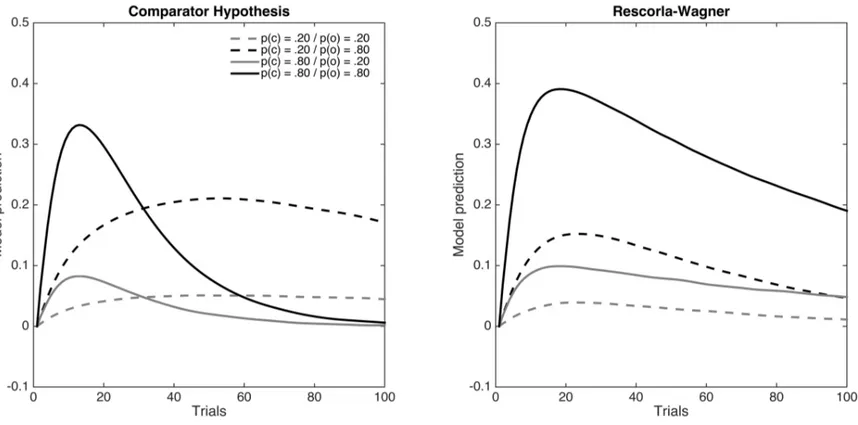
Using this set of equations, it is easy to show that the Comparator Hypothesis predicts both the cue- and outcome-density effects explained in previous sections of this paper. For illustrative purposes, Figure 1 shows the predictions of the model in four
different conditions where the probability of the outcome and the probability of the cue are manipulated orthogonally (taken from Blanco et al., 2013). As can be seen, the Comparator Hypothesis predicts that responding to the target cue should always be higher for
conditions with P(o) = .80 than for their equivalent counterparts with P(o) = .20. In other words, the Comparator Hypothesis predicts the outcome-density bias.
The predictions regarding the cue-density bias are more complex. Figure 1 shows that early in the sequence of trials, responding tends to be higher for conditions with P(c) = .80 than for the corresponding conditions with P(c) = .20. However, this trend is reversed
later on during training. That is to say, at least with the parameter values used to produce the simulations depicted in Figure 1, the Comparator Hypothesis predicts a cue-density effect during the initial stages of learning, followed by an anti-cue-density bias.
Exploratory simulations (not reported here) suggest that this trend is observed with any combination of parameters, as long as the salience of the target cue is higher than the salience of the context. The anti-cue-density bias is due to the fact that the association between the target cue and the context develops very slowly when the probability of the cue is low (i.e., when the target cue is usually absent). This, in turn, limits the ability of the context to down-modulate responding to the target cue (see Equation 3).
To the best of our knowledge, the prediction that the strength and direction of the cue-density bias depends on the number of trials is a unique prediction of the Comparator Hypothesis. Just as an example, the right panel of Figure 1 shows the predictions of the Rescorla-Wagner for the same four conditions. The most important difference between this model and the Comparator Hypothesis is that the learning rule depends on global error correction. Specifically, the strength of the association between stimuli 1 (i.e., the cue or the context) and 2 (i.e., the outcome) changes according to the equation
ΔV1,2 = s1 · s2 · (λ – ∑Vi,2) (4)
where all the symbols have the same meaning as in Equation 2 and ∑Vi,2 refers to the associative strength of all the predictors of stimulus 2 that are present in that trial.
Importantly, in this implementation of the model, only the associative strengths of stimuli that are actually present change on each trial, that is, the associative strength of the cue is updated only on cue-present trials. Unlike the Comparator Hypothesis, the Rescorla-Wagner model does not incorporate a response production rule analogous to Equation 3. Consequently, in our simulations of the Rescorla-Wagner model we will assume that participants’ behavior is modeled by the strength of the association between the cue and
the outcome. As shown in Figure 1, this implementation of the Rescorla-Wagner model predicts that cue- and outcome-density biases should be observed at all stages of learning, although they become smaller as training proceeds and learning approaches the asymptote (zero, in the case of all four conditions simulated in Figure 1).
Interestingly, in a recent re-analysis of the data reported by Blanco et al. (2013; see Vadillo, Blanco, Yarritu, & Matute, 2016) we have found some evidence of an anti-cue-density bias. The main dependent variable collected by Blanco et al. (2013) was a
numerical rating requested to all participants at the end of training. The analyses conducted on these ratings revealed only a small cue-density bias that disappeared in some conditions. However, in a more recent paper we re-analysed an alternative measure of participants’ perception of contingency between cue and outcome. Specifically, Blanco et al. (2013) requested all participants to predict on each trial whether the outcome would be present or not. Using these binary responses, it is possible to measure participants’ perception of contingency by checking whether the proportion of “yes” responses was higher in trials in which the cue was present than in trials in which the cue was absent (e.g., Allan et al., 2005; Collins & Shanks, 2002). In other words, the difference between P(“yes”|cue) and P(“yes”|no cue), an index known as ΔPpred, can be taken as a measure of the extent to which each participant believes that the cue is a good predictor of the outcome. Using this alternative variable as a dependent measure, Vadillo et al. (2016) re-analysed the data collected by Blanco et al. (2013) and observed that in some conditions participants actually showed an anti-cue-density bias. Given that the two experiments conducted by Blanco et al. (2013) comprised a relatively long sequence of trials, these data provide some support for the predictions of the Comparator Hypothesis shown in Figure 1.
The previous section shows that the Comparator Hypothesis can account for the cue- and outcome-density biases typically observed in human contingency learning and that it makes novel predictions that receive some support from previous research. In this section, we compare the relative fit of the Comparator Hypothesis and the Rescorla-Wagner model to a large set of studies on cue- and outcome-density effects conducted by the first author and colleagues. Specifically, we used the 20 experimental conditions summarized in Table 1. These data were taken from the re-analysis conducted by Vadillo et al. (2016), from which we only excluded two experimental conditions from Yarritu et al. (2014), because in that experiment each participant was exposed to a unique cue-outcome contingency. As can be seen in Table 1, several of the experimental conditions re-analysed by Vadillo et al. (2016) involved the same experimental design (defined here as the frequencies of each trial type: a, b, c, and d). For the sake of simplicity, in the following analyses data from
comparable experimental conditions were collated using a weighted mean (also shown in Table 1).
We compared the fit of both models to two different dependent variables explored by Vadillo et al. (2016). One of them is ΔPpred (see the previous section). An advantage of these scores is that they are computed on the basis of trial-by-trial predictions, which were collected using exactly the same procedure in all the experiments overviewed by Vadillo et al. (2016). They are also the dependent variable in which we observed an anti-cue-density bias in some conditions, which might play an essential role to discriminate between models. Unfortunately, the use of these scores is not free from problems. Given that they are based on a long series of trial-by-trial predictions, ΔPpred may not reflect accurately participants’ perception of contingency at the end of training. To overcome this problem, we also fitted both models to the numerical judgments of contingency provided by participants at the end of the experiment. These judgments were collected using slightly
different procedures across experiments and, consequently, they are noisier than ΔPpred (Matute et al., 2011; Vadillo, Miller, & Matute, 2005; Vadillo et al., 2011). However, they are more likely to capture participants’ sensitivity to contingency at the end of the
experiment.
We aimed at comparing the relative fit of both models using optimal parameters for each of them (for a similar approach, see Witnauer, Hutchings, & Miller, 2017; Witnauer, Rhodes, Kysor, & Narasiwodeyar, in press). In our implementation of the Comparator Hypothesis, the model has the same number of free parameters as the Rescorla-Wagner model, namely, the saliences of the target cue, sC, the context, sCTX, and the outcome, sO. These parameters play a similar role in both models: They are typically assumed to reflect the amount of attention gathered by each stimulus and they modulate the rate of acquisition of each association. Initially, we attempted to fit the models using only a gradient descent algorithm (MATLAB’s fminsearch function). However, we found that the algorithm returned radically different parameters depending on the starting values, suggesting the presence of multiple local minima. To ameliorate this problem, we adopted a two-step strategy. Firstly, we used a grid-search process, testing the fit of each model with all combinations of parameter values from .10 to .90 in steps of .10. For each of the experimental conditions summarized in Table 1, we estimated the predictions of the models by simulating 1,000 iterations with random trial orders. Model performance was assessed with the root mean squared error (RMSE). Secondly, once the grid-search process ended we used the combination of parameters that yielded the lowest RMSE as starting values for the gradient-descent algorithm. The best-fitting parameters obtained with this combination of methods are presented in Table 2. Although our procedure ensures a comprehensive exploration of the parameter space, we cannot reject categorically the
possibility that these parameter values are local minima. All the MATLAB scripts that we used in our analyses are available at the Open Science Framework (https://osf.io/z9ad7/).
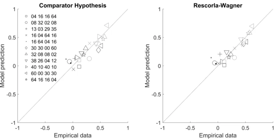
Figure 2 shows the overall fit of both models to the empirical data. Black symbols denote ΔPpred and grey symbols denote judgments. In both panels, data points falling exactly in the diagonal indicate a perfect correspondence between observed and predicted responses. Points above or below the diagonal indicate that the model overestimates or underestimates empirical responses, respectively. The RMSE of each model is shown in Table 2. As can be seen, both models were able to fit ΔPpred and judgments with reasonable accuracy, with the Rescorla-Wagner model achieving a somewhat better fit (ΔRMSE = 0.024 and 0.007 for ΔPpred scores and judgments, respectively).
Alternative Implementations
Although the previous simulations reveal a good fit of both models to the empirical data, it may be possible to improve their performance using alternative and more flexible formalizations of the models. As explained above, our implementation of the Comparator Hypothesis is simpler than the formulation offered by Stout and Miller (2007).
Specifically, (a) we used a slightly different extinction rule (see Footnote 1) and (b) we also ignored, k2, a parameter that down-modulates the impact of the indirect activation of the outcome (i.e., VC,CTX · VCTX,O) on responding. The latter choice, in particular, might have an important impact on the model predictions for our data set, because it determines whether responding is mainly driven by cue-outcome contingency (i.e., as defined by ΔP) or by mere cue-outcome contiguity. That is to say, the model can be made more sensitive to coincidences or to overall contingency by selecting different values for k2.
Consequently, in the present section, we tested the quantitative fit of an alternative
the details of the model were kept as in the previous analyses, except that Equation 3 was rewritten as
R = VC,O – k2 · (VC,CTX · VCTX,O) (4)
where k2 is allowed to vary as a free parameter. To avoid any confusion, henceforth we will refer to this alternative implementation of the Comparator Hypothesis as CH-2.
Similarly, since the original publication of the Rescorla-Wagner model, different extensions have been suggested, especially in the area of human contingency learning. For instance, parameter sO is sometimes allowed to take different values in outcome-present and outcome-absent trials (Lober & Shanks, 2000; Wasserman et al., 1993). In the following sections, we refer to this alternative implementation of the model as RW-2. In the same vein, Van Hamme and Wasserman (1994) developed an extension of the
Rescorla-Wagner model that allowed updating the associative strength of absent stimuli by assuming a negative sC in cue-absent trials.
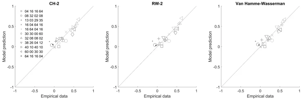
Figure 3 and Table 2 summarize the performance of these alternative
implementations with best-fitting parameters, obtained with the same optimization procedure described in the previous section. Logically, these models achieve better performance than their simpler counterparts because they have an additional free parameter.2 Within these extended models, the Van Hamme-Wasserman algorithm fits ΔPpred scores slightly better than the rest of the models, while CH-2 provides the best overall fit to judgments. Note, however, that these differences are small in terms of RMSE values.
The simpler implementations of the Comparator Hypothesis and the Rescorla-Wagner model cannot be directly compared to their extended counterparts using RMSE as a criterion, because this metric fails to take into account the fact that the latter models include an additional free parameter and, consequently, are less parsimonious. A popular
metric to compare models with different levels of complexity is the Akaike Information Criterion (AIC) which can be computed from RMSE using the equation
AIC = n · log(SSE/n) + 2P (5)
where n is the number of observations (11 in our case), SSE is the sum of squared errors, and P is the number of free parameters (3 or 4 in our case, depending on the model). Models with smaller AICs are preferred to models with higher values. The final term, 2P, ensures that, other things being equal, AICs will be lower for models with fewer free parameters (see Lewandowsky & Farrell, 2010, for more information on the computation and interpretation of AICs).
As can be seen in Table 2, neither CH-2, RW-2 or the Van Hamme-Wasserman model outperform the simple Rescorla-Wagner model in terms of AICs. In other words, although these models achieve a better fit (i.e., lower RMSE), the gains do not pay off when pitted against the loss of parsimony. Interestingly, CH-2 achieves a lower AIC than the simpler version of the Comparator Hypothesis, both for ΔPpred and judgments,
suggesting that parameter k2 plays an essential role in allowing the model to fit the present data set. This does not happen with the extensions of the Rescorla-Wagner model, which perform worse than the original model. Therefore, while k2 seems to improve the fit of the Comparator Hypothesis, neither allowing different values for sC in present and cue-absent trials (Van Hamme & Wasserman, 1994) or allowing different values for sO in outcome-present and outcome-absent trials (Wasserman et al., 1993) seem to improve the fit of the Rescorla-Wagner model.
General Discussion and Concluding Comments
The simulations and model comparisons reported in the previous sections show that the Comparator Hypothesis must be regarded as valid and promising account of biases in
human contingency learning. The Comparator Hypothesis not only predicts that cue- and outcome-density biases should be observed, but also anticipates that the sign and
magnitude of the former depend heavily on the amount of training (see Figure 1). Given that this pattern of results is not predicted by the Rescorla-Wagner model, it is possible to compare the merits of both models by fitting them to a rich dataset with information about people’s ability to detect and rate contingency under conditions with different values of ΔP, P(c), P(o), and number of trials. Using data from 20 experimental conditions (see Table 1) we observed that, in general, both models were able to approximate the actual behavior of participants with a high degree of precision (see Figure 2). Although the Rescorla-Wagner model outperformed the Comparator Hypothesis, the difference between them in terms of RMSE was relatively small. Clearly, the Comparator Hypothesis is a worthy rival of the Rescorla-Wagner model that must be considered in future research.
In our analyses, we also found that extending the Rescorla-Wagner model with additional parameters (i.e., assuming different values of sO for outcome-present and outcome-absent trials or assuming negative values of sC for cue-absent trials) did not improve the fit of the model substantially. Although the RMSE was logically lower for the more complex versions of the Rescorla-Wagner model than for the basic model with just three free parameters, the AICs were actually lower for the simple than for the complex versions. In other words, the improvement in fit does not compensate for the loss of parsimony. In contrast, AICs were lower for CH-2 than for the simpler implementation of the Comparator Hypothesis. This shows that allowing the contribution of the comparator process to be modulated by parameter k2 (see Equation 4) does improve the fit of the model. Even so, the Comparator Hypothesis failed to outperform the Rescorla-Wagner model, either with or without parameter k2.
Of course, these results hinge on the data that we used to fit both models. Although all the experimental conditions included in the present analyses come from the same laboratory, they are representative of the designs used in other studies exploring cue- and outcome-density biases in human contingency learning and they cover a wide range of experimental designs: Within our dataset we included experiments manipulating cue and outcome density with long (e.g., 30/30/0/60) and short (e.g., 8/32/2/8) sequences of trials, and with positive and null cue-outcome contingencies. But however rich, the present dataset does not exhaust the infinite space of combinations of trial frequencies. For instance, none of the experiments included in the present analyses explored cue or
outcome-density biases under negative contingencies. This means that in our analyses most of the empirical data points and model predictions tended to concentrate on the positive side of the contingency spectrum, constraining their variation to a relatively narrow range of values. Similarly, and perhaps more importantly, our data set did not include any
experiment where cue-density and training length were manipulated orthogonally, keeping other factors constant. This is unfortunate because the simulations reported in Figure 1 suggest that such an experiment would offer the best chance to discriminate between the Comparator Hypothesis and the Rescorla-Wagner model. Future research should explore thoroughly this combination of experimental manipulations.
Autor note
MAV was supported by Grant 2016-T1/SOC-1395 from Comunidad de Madrid and Grant PSI2017-85159-P (AIE/FEDER, UE) from Agencia Estatal de Investigación of the Spanish Government and the European Regional Development Fund. MAV would also like to thank the Basque Government for providing the financial support that allowed him to spend three months at Ralph Miller’s lab in 2004. IB was supported by Grant
PSI2016-75776-R (AEI/FEDER, UE) from Agencia Estatal de Investigación of the Spanish
Government and the European Regional Development Fund. Correspondence concerning this article should be addressed to Miguel A. Vadillo, Departamento de Psicología Básica, Facultad de Psicología, Universidad Autónoma de Madrid, 28049 Madrid, Spain. E-mail: [email protected]
References
1. Allan, L. G. (1980). A note on measurement of contingency between two binary variables in judgement tasks. Bulletin of the Psychonomic Society, 15, 147-149. 2. Allan, L. G., & Jenkins, H. M. (1983). The effect of representations of binary
variables on judgment of influence. Learning and Motivation, 14, 381-405. 3. Allan, L. G., Siegel, S., & Tangen, J. M. (2005). A signal detection analysis of
contingency data. Learning & Behavior, 33, 250-263.
4. Barberia, I., Blanco, F., Cubillas, C. P., & Matute, H. (2013) Implementation and Assessment of an intervention to debias adolescents against causal illusions. PLoS ONE, 8, e71303.
5. Blanco, F., Matute, H., & Vadillo, M. A. (2013). Interactive effects of the
probability of the cue and the probability of the outcome on the overestimation of null contingency. Learning & Behavior, 41, 333-340.
6. Buehner, M. J., Cheng, P. W., & Clifford, D. (2003). From covariation to causation: A test of the assumption of causal power. Journal of Experimental Psychology: Learning, Memory, and Cognition, 29, 1119-1140.
7. Bush, R. R., & Mosteller, F. (1951). A mathematical model for simple learning. Psychological Review, 58, 313-323.
8. Chapman, G. B., & Robbins, S. J. (1990). Cue interaction in human contingency judgment. Memory & Cognition, 18, 537-545.
9. Cheng, P. W., & Novick, L. R. (1992). Covariation in natural causal induction. Psychological Review, 99, 365-382.
10. Collins, D. J., & Shanks, D. R. (2002). Momentary and integrative response strategies in causal judgment. Memory & Cognition, 30, 1138-1147.
11. Danks, D. (2003). Equilibria of the Rescorla–Wagner model. Journal of Mathematical Psychology, 47, 109-121.
12. Denniston, J. C., Savastano, H. I., & Miller, R. R. (2001). The extended comparator hypothesis: Learning by contiguity, responding by relative strength. In R. R.
Mowrer & S. B. Klein (Eds.), Handbook of contemporary learning theories (pp. 65-117). Hillsdale, NJ: Erlbaum.
13. Griffiths, T. L., & Tenenbaum, J. B. (2007). From mere coincidences to meaningful discoveries. Cognition, 103, 180-226.
14. Jenkins, H. M., & Ward, W. C. (1965). Judgment of contingency between responses and outcomes. Psychological Monographs, 79, 1-17.
15. Johansen, M. K., & Osman, M. (2015). Coincidences: A fundamental consequence of rational cognition. New Ideas in Psychology, 39, 34-44.
16. Kamin, L. J. (1968). “Attention-like” processes in classical conditioning. In M. R. Jones (Ed.), Miami symposium on the prediction of behavior: Aversive stimulation (pp. 9-31). Miami, FL: University of Miami Press.
17. Kao, S.-F., & Waserman, E. A. (1993). Assessment of an information integration account of contingency judgment with examination of subjective cell importance and method of information presentation. Journal of Experimental Psychology: Learning, Memory, and Cognition, 19, 1363-1386.
18. Levin, I. P., Wasserman, E. A., & Kao, S.-F. (1993). Multiple methods for examining biased information use in contingency judgments. Organizational Behavior and Human Decision Processes, 55, 228-250.
19. Lewandowsky, S., & Farrell, S. (2010). Computational modeling in cognition: Principles and practice. Sage Publications.
20. Lilienfeld, S. O., Ritschel, L.A., Lynn, S. J., Cautin, R. L., & Latzman, R. D. (2014). Why ineffective psychotherapies appear to work: A taxonomy of causes of spurious therapeutic effectiveness. Perspectives on Psychological Science, 9, 355-387.
21. Lober, K., & Shanks, D. R. (2000). Is causal induction based on causal power? Critique of Cheng (1997). Psychological Review, 107, 195-212.
22. López, F. J., Cobos, P. L., Caño, A., & Shanks, D. R. (1998). The rational analysis of human causal and probability judgment. In M. Oaksford & N. Chater (Eds.), Rational models of cognition (pp. 314–352). Oxford, UK: Oxford University Pres. 23. Mackintosh, N. J. (1975). A theory of attention: Variations in the associability of
stimuli with reinforcements. Psychological Review, 82, 276-298.
24. Matute, H., Blanco, F., Yarritu, I., Díaz-Lago, M., Vadillo, M. A., & Barberia, I. (2015). Illusions of causality: How they bias our everyday thinking and how they could be reduced. Frontiers in Psychology, 6:888.
25. Matute, H., Yarritu, I., & Vadillo, M. A. (2011). Illusions of causality at the heart of pseudoscience. British Journal of Psychology, 102, 392-405.
26. Mckenzie, C. R. M., & Mikkelsen, L. A. (2007). A Bayesian view of covariation assessment. Cognitive Psychology, 54, 33-61.
27. Miller, R. R., & Matzel, L. D. (1988). The comparator hypothesis: A response rule for the expression of associations. In G. H. Bower (Ed.), The psychology of
learning and motivation (Vol. 22, pp. 51-92). San Diego, CA: Academic Press. 28. Moreno-Fernández, M. M., Blanco, F., & Matute, H. (2017). Causal illusions in
children when the outcome is frequent. PLoS ONE, 12, e0184707.
29. Msetfi, R. M., Murphy, R. A., Simpson, J., & Kornbrot, D. E. (2005). Depressive realism and outcome density bias in contingency judgments: The effect of the
context and intertrial interval. Journal of Experimental Psychology: General, 134, 10-22.
30. Musca, S. C., Vadillo, M. A., Blanco, F., & Matute, H. (2010). The role of cue information in the outcome-density effect: evidence from neural network
simulations and a causal learning experiment. Connection Science, 22, 177-192. 31. Perales, J. C., Catena, A., Cándido, A., & Maldonado, A. (2017). Rules of causal
judgment: Mapping statistical information onto causal beliefs. In M. R. Waldmann (Ed.), The Oxford Handbook of causal reasoning (pp. 29-51). New York: Oxford University Press.
32. Perales, J. C., Catena, A., Shanks, D. R., & González, J. A. (2005). Dissociation between judgments and outcome-expectancy measures in covariation learning: A signal detection theory approach. Journal of Experimental Psychology: Learning, Memory, and Cognition, 31, 1105-1120.
33. Perales, J. C., & Shanks, D. R. (2007). Models of covariation-based causal judgment: A review and synthesis. Psychonomic Bulletin & Review, 14, 577-596. 34. Rescorla, R. A. (1968). Probability of shock in the presence and absence of CS in fear conditioning. Journal of Comparative & Physiological Psychology, 66, 1-5. 35. Rescorla, R. A., & Wagner, A. R. (1972). A theory of Pavlovian conditioning:
Variations in the effectiveness of reinforcement and nonreinforcement. In A. H. Black & W. F. Prokasy (Eds.), Classical conditioning II: Current research and theory (pp. 64-99). New York, NY: Appleton-Century-Crofts.
36. Shanks, D. R. (1995). Is human learning rational? Quarterly Journal of Experimental Psychology, 48A, 257-279.
37. Shanks, D. R., & Dickinson, A. (1987). Associative accounts of causality
21: Advances in research and theory (pp. 229–261). San Diego, CA: Academic Press.
38. Stout, S. C., & Miller, R. R. (2007). Sometimes-competing retrieval (SOCR): A formalization of the comparator hypothesis. Psychological Review, 114, 759-783. 39. Vadillo, M. A., Blanco, F., Yarritu, I., & Matute, H. (2016). Single- and
dual-process models of biased contingency detection. Experimental Psychology, 63, 3-19.
40. Vadillo, M. A., Miller, R. R., & Matute, H. M. (2005). Causal and predictive-value judgments, but not predictions, are based on cue–outcome contingency. Learning & Behavior, 33, 172-183.
41. Vadillo, M. A., Musca, S. C., Blanco, F., & Matute, H. (2011). Contrasting cue-density effects in causal and prediction judgments. Psychonomic Bulletin & Review, 18, 110-115.
42. Van Hamme, L. J., & Wasserman, E. A. (1994). Cue competition in causality judgments: The role of nonpresentation of compound stimulus elements. Learning and Motivation, 25, 127-151.
43. Wagner, A. R. (1981). SOP: A model of automatic memory processing in animal behavior. In N. E. Spear & R. R. Miller (Eds.), Information processing in animals: Memory mechanisms (pp. 5-44). Hillsdale, NJ: Erlbaum.
44. Wagner, A. R., Logan, F. A., Haberlandt, K., & Price, T. (1968). Stimulus selection in animal discrimination learning. Journal of Experimental Psychology, 76, 171-180.
45. Wasserman, E. A. (1990a). Attribution of causality to common and distinctive elements of compound stimuli. Psychological Science, 1, 298-302.
46. Wasserman, E. A. (1990b). Detecting response-outcome relations: Toward an understanding of the causal texture of the environment. In G. H. Bower (Ed.), The psychology of learning and motivation (Vol. 26, pp. 27–82). San Diego, CA: Academic Press.
47. Wasserman, E. A., Dorner, W. W, & Kao, S.-F. (1990). Contributions of specific cell information to judgments of interevent contingency. Journal of Experimental Psychology: Learning, Memory, and Cognition, 16, 509-521.
48. Wasserman, E. A., Elek, S. M., Chatlosh, D. L., & Baker, A. G. (1993). Rating causal relations: The role of probability in judgments of response–outcome contingency. Journal of Experimental Psychology: Learning, Memory, and Cognition, 19, 174-188.
49. Wasserman, E. A., Kao, S.-F., Van-Hamme, L. J., Katagiri, M., & Young, M. E. (1996). Causation and association. In D. R. Shanks, K. J. Holyoak, & D. L. Medin (Eds.), The psychology of learning and motivation, Vol. 34: Causal learning (pp. 207–264). San Diego, CA: Academic Press.
50. Watts, A. L., Smith, S. F., & Lilienfeld, S. O. (2015). Illusory correlation. In R. L. Cautin & S. O. Lilienfeld (Eds.), The encyclopedia of clinical psychology. Malden, MA: Wiley & Sons.
51. Witnauer, J. E., Hutchings, R., & Miller, R. R. (2017). Methods for comparing associative models and an application to retrospective revaluation. Behavioural Processes, 144, 20-32.
52. Witnauer, J., Rhodes, J., Kysor, S., & Narasiwodeyar, S. (in press). The sometimes competing retrieval and Van Hamme and Wasserman models predict the selective role of within-compound associations in retrospective revaluation. Behavioural Processes.
53. Yarritu, I., & Matute, H. (2015). Previous knowledge can induce an illusion of causality through actively biasing behavior. Frontiers in Psychology, 6, 389. 54. Yarritu, I., Matute, H., & Vadillo, M. A. (2014). Illusion of control: The role of
Footnotes
1 In our implementation of the Comparator Hypothesis, the amount of unlearning that takes place in extinction trials is modulated by sC · sO. In contrast, in Stout and Miller (2007, Table 1), unlearning in extinction trials is modulated by sC · k1, where k1 is an additional free parameter that only affects unlearning. We decided to remove k1 from our
implementation because this would render the Comparator Hypothesis and the Rescorla-Wagner model equivalent in terms of the number of free parameters. Note that, once k1 is removed, if learning trials are modulated by sC · sO, while unlearning trials are modulated solely by sC, then learning must be slower than unlearning (because these parameters have values between 0 and 1). To overcome this problem, we assumed that both learning and unlearning are modulated by sC · sO. This is also more consistent with the standard implementation of the Rescorla-Wagner model.
2 It is interesting to note that, among the best fitting parameters for RW-2, sO has a higher value on outcome-present trials than on outcome-absent trials. Although it might seem unrealistic to assume that an outcome can have a higher salience when it is absent than when it is present, Lober and Shanks (2000) suggested that this might be a reasonable assumption in experimental tasks in which participants have strong a priori reasons to expect that the outcome will tend to follow the cue.
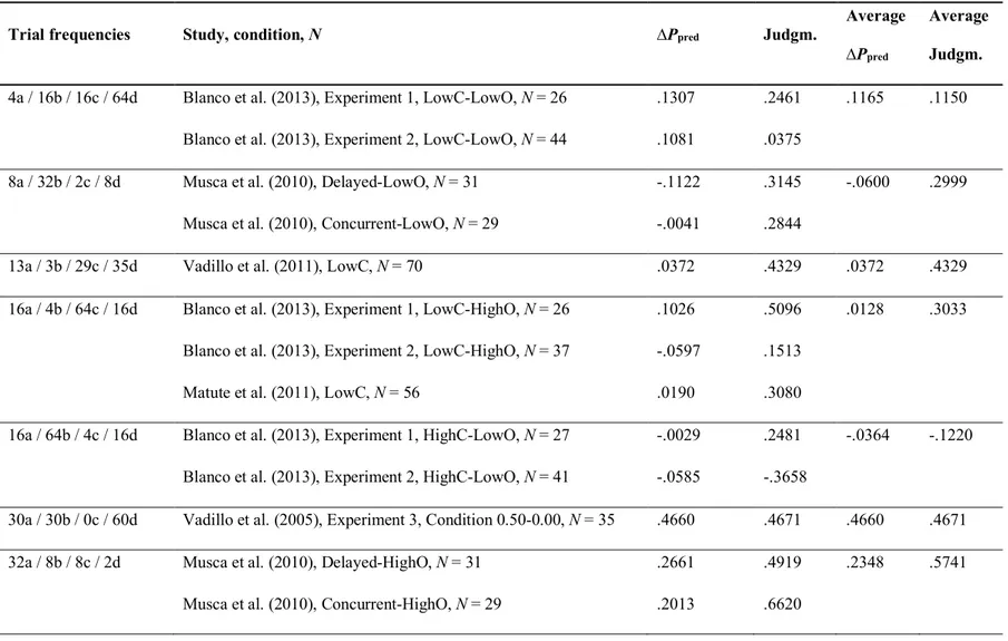
Table 1. Summary of experimental conditions used to fit the models
Trial frequencies Study, condition, N ∆Ppred Judgm.
Average ∆Ppred
Average Judgm.
4a / 16b / 16c / 64d Blanco et al. (2013), Experiment 1, LowC-LowO, N = 26 .1307 .2461 .1165 .1150 Blanco et al. (2013), Experiment 2, LowC-LowO, N = 44 .1081 .0375
8a / 32b / 2c / 8d Musca et al. (2010), Delayed-LowO, N = 31 -.1122 .3145 -.0600 .2999 Musca et al. (2010), Concurrent-LowO, N = 29 -.0041 .2844
13a / 3b / 29c / 35d Vadillo et al. (2011), LowC, N = 70 .0372 .4329 .0372 .4329 16a / 4b / 64c / 16d Blanco et al. (2013), Experiment 1, LowC-HighO, N = 26 .1026 .5096 .0128 .3033
Blanco et al. (2013), Experiment 2, LowC-HighO, N = 37 -.0597 .1513
Matute et al. (2011), LowC, N = 56 .0190 .3080
16a / 64b / 4c / 16d Blanco et al. (2013), Experiment 1, HighC-LowO, N = 27 -.0029 .2481 -.0364 -.1220 Blanco et al. (2013), Experiment 2, HighC-LowO, N = 41 -.0585 -.3658
30a / 30b / 0c / 60d Vadillo et al. (2005), Experiment 3, Condition 0.50-0.00, N = 35 .4660 .4671 .4660 .4671 32a / 8b / 8c / 2d Musca et al. (2010), Delayed-HighO, N = 31 .2661 .4919 .2348 .5741
38a / 26b / 4c / 12d Vadillo et al. (2011), HighC, N = 70 .1587 .4207 .1587 .4207 40a / 10b / 40c / 10d Yarritu & Matute (2015), LowC, N = 53 .0730 .4772 .0730 .4772 60a / 0b / 30c / 30d Vadillo et al. (2005), Experiment 3, Condition 1.00-0.50, N = 32 .5156 .6219 .5156 .6219 64a / 16b / 16c / 4d Blanco et al. (2013), Experiment 1, HighC-HighO, N = 27 .2496 .7017 .1991 .5509
Blanco et al. (2013), Experiment 2, HightC-HighO, N = 38 .1710 .3184
Matute et al. (2011), HighC, N = 52 .2500 .5778
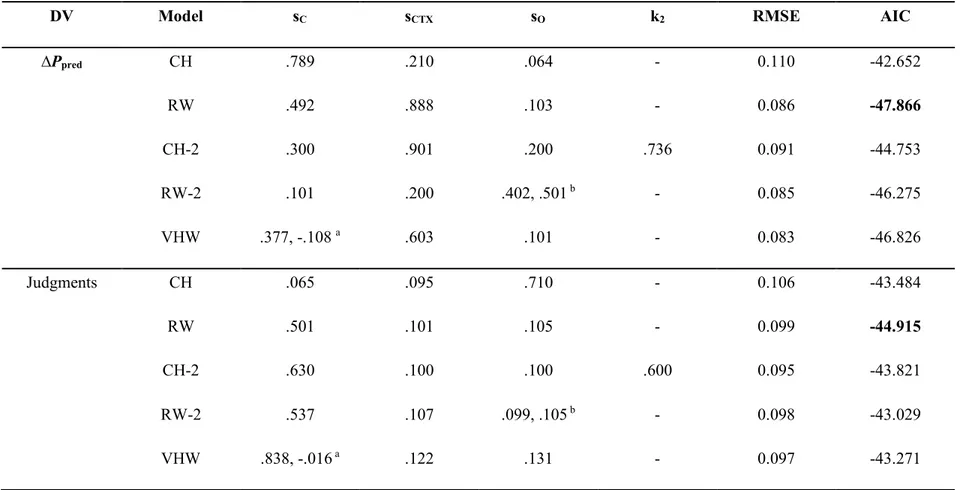
Table 2. Best fitting parameters and summary of model fit
DV Model sC sCTX sO k2 RMSE AIC
∆Ppred CH .789 .210 .064 - 0.110 -42.652 RW .492 .888 .103 - 0.086 -47.866 CH-2 .300 .901 .200 .736 0.091 -44.753 RW-2 .101 .200 .402, .501 b - 0.085 -46.275 VHW .377, -.108 a .603 .101 - 0.083 -46.826 Judgments CH .065 .095 .710 - 0.106 -43.484 RW .501 .101 .105 - 0.099 -44.915 CH-2 .630 .100 .100 .600 0.095 -43.821 RW-2 .537 .107 .099, .105 b - 0.098 -43.029 VHW .838, -.016 a .122 .131 - 0.097 -43.271
Note. DV = dependent variable; sC / sCTX / sO / k2 = best-fitting parameters of the models; RMSE = root mean squared error; AIC = Akaike Information Criterion; CH = Comparator Hypothesis; RW = Rescorla-Wagner model; CH-2 = Comparator Hypothesis with parameter k2; VHW = Van Hamme and Wasserman’s revision of the Rescorla-Wagner model; RW-2 = Rescorla-Wagner model with different values of sO for outcome-present and outcome-absent trials; a sC for cue-present and cue-absent trials, respectively, in VHW; b sO for outcome-present and outcome-absent trials in RW-2.
Figure 1. Predictions of the Comparator Hypothesis and the Rescorla-Wagner model for four different conditions. The learning curve of each
condition is the result of averaging the model’s performance across 5,000 iterations with different (random) trial orders. For both simulations, the parameter values were arbitrarily set to sC = 0.300, sCTX, = 0.200, sO = 0.400. Outcome salience, sO, adopted the same value in outcome-present and outcome-absent trials.
Figure 2. Correspondence between empirical data and predictions of the Comparator Hypothesis and the Rescorla-Wagner model with
best-fitting parameters. Each data point denotes one of the trial-frequency conditions in Table 1. Black symbols denote ∆Ppred and grey symbols denote judgments.
Figure 3. Correspondence between empirical data and predictions of the Comparator Hypothesis with parameter k2 (CH-2), the Rescorla-Wagner model with different sC values for cue-present and cue-absent trials (RW-2), and Van Hamme and Wasserman’s (1994) revision of the Rescorla-Wagner model, all of them with best-fitting parameters. Each data point denotes one of the trial-frequency conditions in Table 1. Black symbols denote ∆Ppred and grey symbols denote judgments.