LIST OF CONTENTS
1. INTRODUCTION ... 3
2. THE UPGRADE OF THE NACIE FACILITY (NACIE-UP): AN OVERVIEW ... 5
2.1. The fuel pin bundle simulator ... 12
2.2. Bundle Instrumentation ... 18
2.3. Data Acquisition and Control System (DACS)... 24
3. EXPERIMENTAL TEST MATRIX ... 27
4. POST-PROCESSING METHOD ... 31
4.1. Definitions and derived quantities ... 31
4.1.1. Bulk temperature and section-averaged wall temperature ... 31
4.1.2. Temperatures across the FPS ... 32
4.1.3. Wall temperature correction ... 33
4.1.4. LBE Mass flow rate ... 35
4.1.5. Non-dimensional numbers ... 35
4.2. LBE physical properties ... 37
4.3. Error analysis method ... 38
5. RESULTS: HEAT TRASFER ANALYSIS ... 39
5.1. Local results ... 40
5.2. Overall heat transfer ... 47
5.3. Coolability of the MYRRHA fuel assembly ... 51
6. CONCLUSIONS ... 54
NOMENCLATURE ... 56
REFERENCES ... 58
7. Annex A ... 59
• INTRODUCTION
In the frame of the research activities planned to support the development of the MYRRHA irradiation facility (SCK-CEN), ENEA assumed the commitment to run experimental tests to simulate the thermal-hydraulic behavior of a wire-spaced fuel pin bundle cooled by heavy liquid metal. These activities, which were performed in the context of the European FP7 SEARCH Project, will support the Front End Engineering Design of the MYRRHA irradiation facility.
The experimental campaign is implemented on the NACIE (NAtural CIrculation Experiment) loop, located at ENEA Brasimone Research Centre, which was instrumented and refurbished to achieve these goals. The Upgraded facility is in the NACIE-UP configuration.
NACIE-UP is a rectangular loop which allows to perform experimental campaigns in the field of the thermal-hydraulics, fluid-dynamics, chemistry control, corrosion protection and heat transfer and to obtain correlations essential for the design of nuclear plant cooled by heavy liquid metals. The primary circuit basically consists of two vertical pipes (O.D. 2.5”), working as riser and downcomer, connected by two horizontal pipes (O.D. 2.5”). Then, the facility consists of an ancillary gas system (for the cover gas and the injection systems) and a pressurized water (16 bar) secondary side for heat removal. Moreover a fill and drain system is installed to allow the right operation of the loop. A full description of the NACIE-UP facility is reported in Section .
The test section for the experiments about the thermal-hydraulic behavior of a wire-spaced fuel pin bundle consists of 19 electrical pins with an active length Lactive = 600 mm. The pin have a diameter D = 6.55 mm, and the maximum wall heat flux will be close to 1 MW/m2. The pins are placed on an hexagonal lattice by a suitable wrapper, while spacer grids will be avoided thanks to the wire spacer. This fuel pin bundle configuration is relevant for the MYRRHA’s core thermal-hydraulic design [1].
The experiment was designed in order to analyze the thermal-hydraulic behavior of the MYRRHA FA during a Loss of Flow Accident (LOFA) with the coast-down of the main circulation pump. Heat transfer during a LOFA is driven by the inertia of the fluid during the pump coast-down and the onset of natural circulation due to the difference in height between the heat source and the heat sink. As a consequence of a LOFA, a stationary natural circulation flow rate will be established in a characteristic time which depends on the specific geometry of the system under consideration and on the geometry of the bundle.
Actually, some differences exist between the MYRRHA bundle and the NACIE-UP bundle. One is the number of ranks and pins: 7 ranks and 127 pins for MYRRHA against 3 ranks and 19 pins for NACIE-UP. This difference in the number of pins is not relevant for the convective heat transfer in the subchannels because side, corner and central subchannels can be monitored in the 19 pin bundle and basic phenomenology is the same as in the MYRRHA bundle. For a fixed average velocity in the bundle, pressure drops are expected to be a little higher in the NACIE-UP bundle because the influence of the wall is stronger, but from the literature and from numerical evidences [2], it is clear that this difference is not really relevant. The subchannel velocity usc determines, on the base of the geometry of the bundle and on the fluid properties, the LBE mass flow rate in the MYRRHA FA
[ / ] FA
side, the linear power density Qlin [kW/m] fixes the total power of the NACIE-UP 19-pin bundle Q[kW].
Actually, the NACIE-UP facility can reach mass flow rates up to ~6 kg/s and both the bundle and the Heat Exchanger are designed for a maximum power of ~250 kW. In practice, this theoretical range is limited by the maximum clad temperature to safely operate the electrical pin Tclad < 550 °C. All these considerations were taken into account into defining the experimental test matrix, described in Section .
In this document, the post-test analyses for the experimental tests are described. A complete description of the post processing methods is reported in Section . The treatment of acquired data and the computation of derived quantities is fully explained. The error treatment method, which is in accordance with the error propagation theory, is also described.
Section shows the main results on heat transfer obtained from the experimental tests performed at ENEA Brasimone Research Centre with the mock-up of the MYRRHA FA placed in the NACIE-UP facility. Different methods for the evaluation of both local and section-averaged heat transfer coefficients are presented. These methods are discussed and the results compared with the correlations existing in literature. Then, the main results on the coolability of the MYRRHA fuel assembly are summarized in Section 5.
• THE UPGRADE OF THE NACIE FACILITY (NACIE-UP): AN OVERVIEW
NACIE-UP is a rectangular loop which allows to perform experimental campaigns in the field of the thermal-hydraulics, fluid-dynamics, chemistry control, corrosion protection and heat transfer and to obtain correlations essential for the design of nuclear plant cooled by heavy liquid metals. It basically consists of two vertical pipes (O.D. 2.5”), working as riser and downcomer, connected by two horizontal pipes (O.D. 2.5”). In the NACIE-UP configuration, the whole height of the facility is about 8 meters, while the horizontal length is about 2,4 m. In the bottom of the riser a prototypical wire-spaced fuel pin bundle simulator (FPS), with a maximum power of 235 kW, have been installed. A proper heat exchanger is placed in the upper part of the downcomer.
NACIE-UP is made in stainless steel (AISI 304) and can use both lead and the eutectic alloy LBE as working fluid (about 2000 kg, 200 l in the updated configuration). It was designed to work up to 550°C and 10 bar. The difference in height between the center of the heating section and the center of the heat exchanger is about 5.5 m, and it is very important for the intensity of the natural circulation. In the riser, an argon gas injection device ensures a driving force to sustain forced convection in the loop.
The reference for the piping and instrumentation is the P&ID reported in Figure 1, where all the instrumentation, components and pipes are listed and logically represented. A schematic layout of the primary circuit is reported in Figure 2.
The facility includes:
• The Primary side, filled with LBE, with 2 ½” pipes. It consists of two vertical pipes , working as riser and downcomer, two horizontal pipes and an expansion tank;
• A new Fuel Pin Simulator (19-pins) 250 kW maximum power, placed in the bottom of the riser of the primary side;
• A Shell and tube HX with two sections, operating at low power (5-50 kW) and high power (50-250 kW). It is placed in the higher part of the downcomer;
• A high mass flow rate induction flow meter (3-15 kg/s) FM102, located in the downcomer, after the HX;
• 5 bubble tubes to measure the pressure drops across the main components and the pipes; • Several bulk thermocouples to monitor the temperature along the flow path in the loop; • The Secondary side, filled with water at 16 bar, connected to the HX, shell side. It includes a
pump, a pre-heater, an air-cooler, by-pass and isolation valves, and a pressurizer (S201) with cover gas;
• An ancillary gas system, to ensure a proper cover gas in the expansion tank, and to provide gas-lift enhanced circulation;
• A LBE draining section, with ½″ pipes, isolaNon valves and a storage tank (S300);
The ancillary gas system is practically identical to the previous configuration of the NACIE facility and does not have significant upgrade. It has the function to ensure the cover gas in S101 and to manage the gas-lift system in the riser (T103) for enhanced circulation regime.
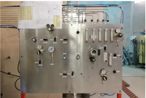
The primary system is ordinary filled with liquid LBE and it is made by several components, pipes and coupling flanges. Pipes T101, T102, T103, T104, T105 are austenitic SS AISI304 2.5″S40, I.D. 62.68 mm. Figure 3 shows a picture of the primary side of the NACIE-UP facility.
Figure.3: NACIE-UP facility.
The main component of the primary loop is the instrumented Fuel Pin Bundle Simulator (FPS-19250), and it is fully described in Sections o and o. Most of the hydraulic resistance of the loop is in the wire-spaced FPS and thus it is very important to correctly measure the pressure drop across it through the F501 and F502 bubble tubes. The isolation 2.5″ ball valve V142, placed downstream the FPS, will protect the FPS during the draining of the facility and will be partially closed to regulate the mass flow rate through the loop.
An expansion tank (S101) is located at the end of the riser and is partially filled with Argon as cover gas to control the pressure inside the primary circuit. Two level sensors LD101, LD102, are located respectively 80 and 180 mm above the outlet nozzle of the riser, inside the expansion vessel. A drawing of the expansion vessel (S101) is reported in Figure.4. Pipe 1 in Figure.4 is welded to the pipe working as riser (T103) and ends with a nozzle 285 mm long inside the tank.
Figure.4: Layout of the expansion vessel inside the primary circuit of the NACIE-UP facility.
The fill and drain system has been designed to be completely controlled by DACS, and the fill and drain operational procedures are fully described in [3]. This system is made of austenitic SS AISI304 1/2″ pipes, isolaNon valves, a filter (T305) and a storage tank (S300). In Figure.5 some components of the fill and drain system are shown.
Figure.5: Sketches of the fill and drain system of the NACIE-UP facility.
In the riser, an argon gas injection device ensures a driving force to sustain enhanced circulation regime in the loop. The gas injection system is composed of a 9 mm I.D. pipe inserted inside the riser and is connected to the ancillary gas system. The pipe is 6135 mm long starting from the 2 ½” coupling flange in the upper part expansion tank and ends with a 4.35 mm I.D. hook-shaped pipe. More details on the operation of the gas injection system are described in [4].
The flow meter FM102 is based on the magnetic induction effect and is accurate for relatively ‘high’ mass flow rates (5-20 kg/s). FM102 has been tested in the last configuration of NACIE in December 2012 and results are documented in [5].
The secondary side is a 16 bar pressurized water loop, with a circulation pump PC201, a pre-heater H201, the HX shell side, an air-cooler E201 and a pressurizer S201. Components of the secondary side are depicted in Figure.6. The pressurizer is connected to the gas lines to ensure an Argon cover gas and to regulate the loop pressure though DACS. Most of the valves are motorized in order to ensure the full operability of the secondary loop by DACS. The valve system allows to drain and fill the two sections of the HX shell separately from the control room. A bypass of the HX is ensured by V214 for the pre-heating of the secondary water. The heating section H201 allows to heat-up the
secondary fluid to have flexibility in managing low FPS powers. The ultrasonic flow meter FM201 allows to monitor the secondary water mass flow rate, while several thermocouples will monitor temperature in the loop; the combination of the two information will allow to quantify the power exchange in the HX. The heat exchanger is shell and tube type and has been designed to exchange heat up to 250 kW. Two separated shell sections have been built: a counter-current high-power section (0-30 kW) and a cross-flow low power section (30-250 kW), both connected to the pressurized water secondary side. The two sections can be drained and filled separately. More details about the Shell and tube HX are provided in [6], while the operational process and procedures are of the secondary side are documented in [3].
o The fuel pin bundle simulator
The FPS will consist of 19 electrical pins with an active length Lactive = 600 mm. The whole length (Ltotal = 2000 mm) includes the non-active length and the electrical connectors. The pin have a diameter D=6.55 mm, and the maximum wall heat flux will be close to 1 MW/m2. The pins will be placed on an hexagonal lattice by a suitable wrapper, while spacer grids will be avoided thanks to the wire spacer. The maximum power of the new fuel pin bundle is ~ 235 kW. To simulate the fuel pins, an electrically heated rod bundle has been specifically designed and provided by THERMOCOAX for this purpose. This fuel pin bundle configuration is relevant for the MYRRHA’s core thermal-hydraulic design [1].
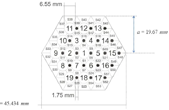
Some dimensions of the fuel bundle and an overall sketch of the cross section are reported in Figure.8.
Figure 7: Cross-section of the electrical wire-spaced fuel pin bundle simulator to be used at ENEA.
The main geometrical dimensions to be considered for a thermal-hydraulic assessment of the FA are:
• The rod diameter D=6.55 mm; • The wire diameter d=1.75 mm;
• The pitch to diameter ratio P/D=(D+d+δ)/D=1.2824, which keeps into account the nominal gap between the wire and the neighbor pins δ=0.1 mm;
• The distance between the last rank of pins and the internal wall of the wrap
δw=d+δ =1.75+0.1 mm= 1.85 mm;
• Wires are helicoidally twisted around each pin with a streamwise pitch of Pw=262 mm; • The regular lattice is triangular/hexagonal staggered.
The total flow area can be conventionally divided into 54 subchannels of different ranks (S1-S54). Pins and subchannels have been numbered to better define the instrumentation needed as well as the physical phenomena involved. The subchannels and the relative pins that will be instrumented are also indicated in Figure.8. Details about the fuel pin bundle instrumentation are described in Section o.
• Figure.8: Sketch fuel pin bundle simulator for the NACIE facility. Instrumented pins in red; instrumented subchannels in orange, wire in black.
The internal dimension of the wrap can be computed by keeping into account that the apothem a of the internal walls of the hexagonal wrapper.
3
2 19.674
2 2
D
a= P + + + =d δ mm (1)
The side length l is simply l=2 / 3a =22.7178mm. In such a way the dimensions of the wrap are fixed according to what required by the MYRRHA FA design.
The geometry shown in Figure 7 allows to study and characterize heat transfer and fluid flow during a LOFA for three different ranks of rods in the MYRRHA FA:
• the external rank N, represented by the pins 8-19 and by subchannels S25-S54; • the rank N-1, represented by pins 2-7 and by subchannels S7-S24;
• the central rank, represented by the central pin n. 1 and by subchannels S1-S6;
These three ranks are representative of all the subchannels in the MYRRHA FA. In fact, it is well known from the literature that for wire-wrapped bundles of similar geometry, the influence of the wall is considered important for the external rank N and for the N-1 rank of pins, while the other ranks are not so much influenced by the wrap wall. Moreover, in principle, the 19-pins bundle will allow to distinguish between the corner pins like 9 or 11 and the pure N rank pins like 10 or 12. The equivalent diameter of such configuration can be easily computed, by keeping into account that the cross-sectional area of the hexagonal wrap is 32 3 / 2
wrap
A = l , while the total area of the pins and the wire is respectively 2
/ 4
pins
A =M Dπ , 2/ 4
wire
the pins. The wetted perimeter is Lw =M
(
πD+πd)
+6l. The resulting equivalent diameter can be computed as:4( )
4.147
wrap pins wire eq w A A A D mm L − − = = (2)
which is slightly higher than the nominal equivalent diameter Deq nom, ≈3.86mm of an infinite lattice with the same geometrical features. However, the influence of the wall on this parameter is quite small for a 19-pins bundle. The nominal equivalent diameter will be used to define the non-dimensional quantities in the post-processing of the results, as agreed with SCK [7].
Several dimensionless groups can be defined on the facility to characterize the thermal-hydraulic phenomena involved. Calling by u the average velocity in the 2.5” tube of diameter dt and section A, a tube Reynolds number can be defined as:
Re t
tube
u d
ν
= (3)
This number gives a first reference for the convective heat transfer. The velocity u, and thus the overall mass flow rate mɺ =ρuAcan be generated both by natural circulation, i.e. by buoyancy forces, and by forced circulation, i.e. by some source of momentum like a pump or the gas-lift injection system.
The role of the natural circulation is expressed by the Grashof number: 2 2 3 2 2 2 bv v H g TH Gr β ν ν ∆ = = (4)
The typical Brunt-Vaisala velocity of the gravity waves can be recognized as vbv= 2gβ∆TH and
represents the velocity of a grave in the modified buoyancy gravity field gβ∆T.
The streamwise subchannel velocity usc in the bundle subchannel, can be computed considering that the mass flow rate is constant in all the sections of the loop, and thus:
3085.567
4.711 654.965
sc
wrap pins wire
A
u u u u
A A A
= ⋅ = ⋅ = ⋅
− − (5)
The subchannel Reynolds number can therefore be computed as:
4.711 Re sc eq eq t 0.290 Re sc tube u D D u d dt ν ν ⋅ ⋅ = = = ⋅ (6)
The subchannel Reynolds number Resc is about 1/3 of the pipe Reynolds number Retube in NACIE-UP
loop.
Pressure losses in the NACIE facility can be estimated via literature known correlations. Losses in the pin bundle appears the most important ones. Referring the global resistance coefficient K to the velocity u in the NACIE 2.5” pipe, it is possible to write K by the formula:
tubes conc bundle
where Ktubes refers to the losses in the loop pipes (horizontal and vertical branches), Kconc refers to the concentrated losses (i.e. elbows, expansion vessel and heat exchanger), Kbundle refers to the bundle losses. Details about formulas used to calculate the pressure losses in the fuel pin simulator bundle and in the whole NACIE-UP loop are mentioned in [6].
The overall layout of the fuel pin bundle simulator is depicted in Figure.9. It consists of the hexagonal wrap and additional parts and flanges to connect the bundle to the NACIE facility. The design pressure is 10 bar and the design temperature is 550°C. The lower non-active region of the bundle is more than 500 mm for thermal hydraulic reasons. A fully developed flow is required into the active zone inlet section for a proper run of the experiment. On the pin foot, a bottom grid is positioned to keep the bundle tight. Referring to the overall bundle layout, the conical portion allows the elastic bending of the pins which should be needed to allow the proper installation of the electrical connectors. All details regarding the components of the fuel pin bundle simulator and the wire installation around the pins can be found in [6].The overall picture of the fuel pin bundle assembled, before the installation in the NACIE-UP facility, is shown in Figure.10.
o Bundle Instrumentation
As already pointed out, Figure.8 represents a section, viewed from the top, of the bundle with pins and subchannels that must be instrumented.
Prototypical pins were already manufactured by THERMOCOAX for ENEA with the specification mentioned above for the LOFA experiment on the coolability of MYRRHA FA.
Pins 2, 4, 6, 7, 9, 16, 18, 19 are equipped with wall embedded thermocouples on a generatrix parallel to the pin axis, as shown in Figure.11. Three different levels will be considered: z= 38, 300, 562 mm starting from the beginning of the active region of the pins (connector side). Conventionally, measurement sections at z=38, 300 and 562 mm will be called respectively section A, B and C. The reference section in Figure 7 is referred at the section A, z=38 mm, and the other measurement sections chosen B, C (i.e. z=300, 562 mm) are exactly in the same configuration, being the wire pitch Pw=262 mm= 300-38 mm= 562-300 mm. Therefore this choice allows to have three independent measurements of heat transfer referred to the same relative position of wire and pins and this feature drops off systematic errors.
Figure.11: Wall Embedded TCs locations for pins n. 2,4,6,7,9,16,18,19.
Pin 1 is instrumented with wall embedded thermocouples on two generatrices a and b, located 180° each other, parallel to the pin axis, pin n. 5 will be instrumented along three generatices a, c, d, located at 120° each other, as it is shown in Figure 12.
Figure.12: Wall Embedded TCs locations for pin n. 1 and n.5
Subchannels S2, S5, S22, S26, S33 are instrumented with bulk thermocouples 0.5 mm thickness at the 3 measurement sections A, B and C, i.e. at levels z=38, 300, 562 mm. The generic measurement section, with wall thermocouples and subchannels instrumented, is shown in a schematic view in Figure.13. The relative position of the grooves, i.e. of the generatrices (marked in red) for the different pins can be also deduced, considering the reference for the azimuthal pin angle ϑ, with positive angles anticlockwise with the bundle section seen from the top.
Figure.13: Generic measurement section (z=38, 300, 562 mm) conventionally view from the top, with the location of wall TCs and instrumented channels.
The related azimuthal angles ϑ are reported in Table 1 for all measurement sections (z=38 mm, z=300 mm, and z=562 mm).
The bulk thermocouples run following the wire associated to the pin closest to the monitored subchannel. The association table between monitored subchannel and wire to be used to allocate bulk thermocouples with other relevant information is reported in Table 2 for the whole bundle.
Table.1: Azimuthal angles of the pin generatrices where the wall embedded Thermocouples are located.
ϑϑϑϑ[°] wall TCs [mm] 1 -60, +120 z= 38, 300, 562 6 0.35 2 +60 z= 38, 300, 562 3 0.35 3 0 z=38, 81.7, 125.3, 169, 212.7, 256.3,300, 343.7, 387.3, 431, 474.7, 518.3, 562 13 0.35 4 0 z= 38, 300, 562 3 0.35 5 -120,0,+120 z= 38, 300, 562 9 0.35 6 +120 z= 38, 300, 562 3 0.35 7 +180 z= 38, 300, 562 3 0.35 9 -120 z= 38, 300, 562 3 0.35 16 -120 z= 38, 300, 562 3 0.35 18 -60 z= 38, 300, 562 3 0.35 19 +60 z= 38, 300, 562 3 0.35
Table.2: Azimuthal angles of the generatrices where the bulk Thermocouples are located for each subchannel instrumented.
Subchannel number
Pin (wire) number
Azimuthal angle ϑϑϑϑ[°] Location [mm] Number of bulk TCs TC diameter [mm] S5 1 +120 z= 38, 300, 562 3 0.5 S2 2 +60 z= 38, 300, 562 3 0.5 S22 6 +120 z= 38, 300, 562 3 0.5 S33 9 -120 z= 38, 300, 562 3 0.5 S26 19 +60 z= 38, 300, 562 3 0.5
Pin number 3 is instrumented along a generatrix with 13 wall embedded thermocouples along the active length, placed every Pw/6=43.66 mm starting from z=38 mm; the azimuthal orientation of the groove is ϑ = 0.
The total number of wall embedded thermocouples is 52. Regarding the bulk thermocouples, they must be placed on 5 subchannels (S2, S5, S22, S26, S33) in 3 different sections (A, B and C, i.e. z=38, 300 and 562 mm) for a total number of bulk thermocouples of 15.
At each measurement section, wall embedded thermocouples must move azimuthally around the pin to reach the correct position/generatrix represented in Figure 13 and reported from Table 1 to Table
3. On the other side, at each measurement section, bulk thermocouples must leave the wire and reach the center of the subchannel to monitor.
To increase the mechanical resistance of the bulk thermocouples placed into the LBE stream, and aiming to guarantee the correct position of them during the run of the experiment, the “prolonged” thermocouples type are adopted. That solution consist of to put the hot junction in the center of the monitored subchannel and to prolong the TC wire to form an arc (thus increasing its stiffness) and then to fix the TC head to the spacing wire by point welding.
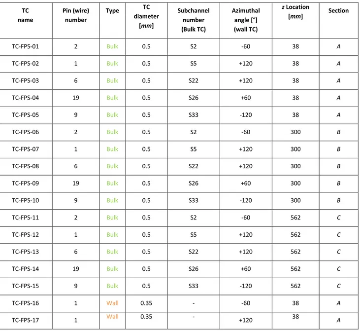
Table 3 provides all the relevant information associated with the thermocouples, i.e. the Pin/wire number, the TC type (‘Wall’ or ‘Bulk’), the TC diameter, the subchannel number for bulk TCs, the azimuthal angle, the vertical z location from the beginning of the active region and the corresponding measurement section ‘A’, ‘B’, or ‘C’. In the cells where the information is not well defined the symbol ‘-‘ is used.
All the thermocouples adopted in the FPS are 'K' type pre-calibrated by the manufacturer (THERMOCOAX) with a certified accuracy of 0.1 K.
Table 3: Thermocouples names with all the relevant information associated.
TC name Pin (wire) number Type TC diameter [mm] Subchannel number (Bulk TC) Azimuthal angle [°] (wall TC) z Location [mm] Section TC-FPS-01 2 Bulk 0.5 S2 -60 38 A TC-FPS-02 1 Bulk 0.5 S5 +120 38 A TC-FPS-03 6 Bulk 0.5 S22 +120 38 A TC-FPS-04 19 Bulk 0.5 S26 +60 38 A TC-FPS-05 9 Bulk 0.5 S33 -120 38 A TC-FPS-06 2 Bulk 0.5 S2 -60 300 B TC-FPS-07 1 Bulk 0.5 S5 +120 300 B TC-FPS-08 6 Bulk 0.5 S22 +120 300 B TC-FPS-09 19 Bulk 0.5 S26 +60 300 B TC-FPS-10 9 Bulk 0.5 S33 -120 300 B TC-FPS-11 2 Bulk 0.5 S2 -60 562 C TC-FPS-12 1 Bulk 0.5 S5 +120 562 C TC-FPS-13 6 Bulk 0.5 S22 +120 562 C TC-FPS-14 19 Bulk 0.5 S26 +60 562 C TC-FPS-15 9 Bulk 0.5 S33 -120 562 C TC-FPS-16 1 Wall 0.35 - -60 38 A TC-FPS-17 1 Wall 0.35 - +120 38 A
TC-FPS-18 2 Wall 0.35 - +60 38 A TC-FPS-19 4 Wall 0.35 - 0 38 A TC-FPS-20 5 Wall 0.35 - -120 38 A TC-FPS-21 5 Wall 0.35 - 0 38 A TC-FPS-22 5 Wall 0.35 - +120 38 A TC-FPS-23 6 Wall 0.35 - +120 38 A TC-FPS-24 7 Wall 0.35 - +180 38 A TC-FPS-25 9 Wall 0.35 - -120 38 A TC-FPS-26 16 Wall 0.35 - -120 38 A TC-FPS-27 18 Wall 0.35 - -60 38 A TC-FPS-28 19 Wall 0.35 - +60 38 A TC-FPS-29 1 Wall 0.35 - -60 300 B TC-FPS-30 1 Wall 0.35 - +120 300 B TC-FPS-31 2 Wall 0.35 - +60 300 B TC-FPS-32 4 Wall 0.35 - 0 300 B TC-FPS-33 5 Wall 0.35 - -120 300 B TC-FPS-34 5 Wall 0.35 - 0 300 B TC-FPS-35 5 Wall 0.35 - +120 300 B TC-FPS-36 6 Wall 0.35 - +120 300 B TC-FPS-37 7 Wall 0.35 - +180 300 B TC-FPS-38 9 Wall 0.35 - -120 300 B TC-FPS-39 16 Wall 0.35 - -120 300 B TC-FPS-40 18 Wall 0.35 - -60 300 B TC-FPS-41 19 Wall 0.35 - +60 300 B TC-FPS-42 1 Wall 0.35 - -60 562 C TC-FPS-43 1 Wall 0.35 - +120 562 C TC-FPS-44 2 Wall 0.35 - +60 562 C TC-FPS-45 4 Wall 0.35 - 0 562 C TC-FPS-46 5 Wall 0.35 - -120 562 C
TC-FPS-47 5 Wall 0.35 - 0 562 C TC-FPS-48 5 Wall 0.35 - +120 562 C TC-FPS-49 6 Wall 0.35 - +120 562 C TC-FPS-50 7 Wall 0.35 - +180 562 C TC-FPS-51 9 Wall 0.35 - -120 562 C TC-FPS-52 16 Wall 0.35 - -120 562 C TC-FPS-53 18 Wall 0.35 - -60 562 C TC-FPS-54 19 Wall 0.35 - +60 562 C TC-FPS-55 3 Wall 0.35 - 0 38 A TC-FPS-56 3 Wall 0.35 - 0 81.7 - TC-FPS-57 3 Wall 0.35 - 0 125.3 - TC-FPS-58 3 Wall 0.35 - 0 169 - TC-FPS-59 3 Wall 0.35 - 0 212.7 - TC-FPS-60 3 Wall 0.35 - 0 256.3 - TC-FPS-61 3 Wall 0.35 - 0 300 B TC-FPS-62 3 Wall 0.35 - 0 343.7 - TC-FPS-63 3 Wall 0.35 - 0 387.3 - TC-FPS-64 3 Wall 0.35 - 0 431 - TC-FPS-65 3 Wall 0.35 - 0 474.6 - TC-FPS-66 3 Wall 0.35 - 0 518.3 - TC-FPS-67 3 Wall 0.35 - 0 562 C
o Data Acquisition and Control System (DACS)
Data acquisition and instrumental control is fully achieved with the aim of LabVIEW System Design Software [8]. The primary and the secondary sides of the NACIE-UP facility can be remotely controlled. The operations of fill and drain of the plant can be made remotely as well. The ancillary gas system, instead, is directly controlled through the gas panel shown in Figure.14.
Figure.14: Manual panel for the gas system control
Figure 15shows the control and monitoring panel to remotely actuate components and valves. From this panel, temperatures and pressures inside the primary and secondary systems can be monitored. In Figure.16 the remote control panel for the activation and the regulation of the power production can be seen. Power level ,number of pin activated and power ramp can be regulated as needed. Moreover, all the wall and bulk thermocouples inside the fuel pin bundle simulator can be constantly monitored from the panel displayed in Figure 17. Each pin can be controlled separately and this feature gives the opportunity to perform asymmetric heating tests for code validation. Ramps from a power level to another one are also possible.
Figure.15: Remote control panel of the NACIE-UP facility
• EXPERIMENTAL TEST MATRIX
The experimental campaign planned at ENEA with the NACIE-UP facility is set in the frame of the research activities to support the development of the MYRRHA irradiation facility (SCK-CEN). The FPS test section, described in Sections o and o, was appropriately manufactured to simulate the thermal-hydraulic behavior of a wire-spaced fuel pin bundle cooled by heavy liquid metal.
The aim of the experimental campaign is to obtain primarily stationary conditions in the facility and to characterize each stationary condition with respect to the local heat transfer measurements in the bundle, the mass flow rate, the pressure drop.
The experimental test matrix range to be performed in the next NACIE-UP campaign was provided by SCK-CEN. The expected test matrix included different power levels. For each power level, different mass flow rates are foreseen. Moreover, in the original SCK-CEN matrix in [9] most of the cases are repeated with two inlet temperatures: Tinlet=200, 270 °C. Nevertheless, as a first approximation, inlet temperature was not regarded, being the thermal-fluid dynamic behavior of the bundle independent by Tinlet.
The reference quantities for each test are: the average subchannel velocity usc [m/s], which characterize the flow from an hydraulic point of view, and the average linear power in a single pin Qlin [kW/m], which defines the heat transfer boundary conditions. The subchannel velocity usc determines, on the base of the geometry of the bundle and on the fluid properties, the LBE mass flow rate in the MYRRHA FA mɺFA [kg s/ ], and the LBE mass flow rate in the NACIE-UP bundle
[ / ] NACIE
mɺ kg s , depending on the flow area of the fuel assembly On the other side, the linear power density Qlin [kW/m] fixes the total power of the NACIE-UP 19-pin bundle Q [kW].
The range of parameters expected in the experimental test matrix provided by SCK-CEN is reported in Table.4
Table.4: Range of parameters for the expected test matrix provided by SCK-CEN.
FLOW
REGIME usc[m s/ ] mɺFA[kg s/ ] mɺNACIE [kg s/ ] ∆ °T C[ ] QNACIE[kW] Qlin[kW m/ ] NC 0.05 – 0.30 2.30 – 11.70 0.4 – 1.8 50-230 10-35 0.9 – 2.9
FC 0.13 – 0.80 5.00 – 31.00 0.9 – 5.4 30 - 210 22 - 110 1.9 – 9.5
For the NACIE-UP facility, the range of mass flow rate that can be in the achieved in pure natural circulation flow is mɺNACIE ≈0.5 1.5− kg s/ , which corresponds to subchannel velocities
0.1 0.25 / sc
u ≈ − m s. The range of subchannel Reynolds number in this case is Resc ≈2000−5000.
In the regime of enhanced circulation, the gas injection system provides additional pressure head and allows to achieve mass flow rates up to mɺNACIE ≈6kg s/ , corresponding to subchannel velocities up to usc ≈0.9m s/ . The maximum value of subchannel Reynolds number achievable is of about Resc ≈20000.
Reynolds number range and subchannel velocities reproducible in NACIE and power range of the heaters agrees with the range required in the MYRRHA HTC specifications document by SCK.
In the NACIE-UP facility, both the bundle and the Heat Exchanger are designed for a maximum power of ~250 kW. Therefore, stationary conditions can be reached in the limits
6 / , 250
NACIE
mɺ < kg s Q< kW . This theoretical range is limited by the maximum clad
temperature to safely operate the electrical pin Tclad <550-600 °C. The Fuel Pin Simulator is operated with a fuel pin protection system which automatically switches off the electric power when at least one of the wall temperatures exceeds the chosen limit. The Tclad limit criterion is practically satisfied if the temperature drop across the bundle is ∆T < 250 °C, and this implies a maximum power to the bundle Qmax =mɺNACIEcp∆Tmax as a practical criterion for the operation of NACIE-UP.
The experimental test matrix performed considers a range power level included between 10 and 110 kW. It corresponds to linear power between 0.9 and 10 kW/m. For each power level, several mass flow rates are taken into account. At first, the case in pure natural circulation flow is attempted. Then, other tests, at lower mass flow rate are essayed, through a partial closure of the valve V142. Additional tests are performed at higher mass flow rates, by setting different flow rates of the gas injected in the riser of the primary system, just downstream the FPS test section. The experimental test matrix with all the cases performed is reported in Table.5. Reynolds and Péclet numbers in Table.5 are computed from the average temperature in the fuel bundle.
Table.5: Experimental test matrix of the performed cases.
PEC TEST NUMBER Q[kW] mNACIEUP[kg/s] mMYRRHAFA[kg/s] Resc∙10-3 Pesc
P99 11 2.92 16.7 7.08 236 P100 11 2.28 13.07 5.45 188 P11X0 11 1.06 6.10 2.72 84 P102 11 0.72 4.08 1.93 55 P102b 11 0.68 3.86 1.84 51 103 11 0.36 2.07 1.13 26 P202 20 4.17 23.92 10.65 332 P203 20 3.10 17.86 8.09 245 P20X0 20 1.49 8.58 4.01 116 P204 20 0.73 4.20 2.24 52 P28X0 28 1.17 6.74 3.69 83 P212 36 3.33 19.18 10.06 242 P213 36 2.22 12.79 6.88 159 P214 36 1.15 6.62 3.96 77 P217 43 3.2 18.43 9.98 228 P218 43 2.8 16.13 8.75 199 P43X0 43 1.62 9.33 5.35 111 P223 52 3.40 19.47 10.81 237 P224 52 2.24 12.79 7.44 151 P265 54 3.23 18.49 10.21 226
P269 108 3.95 22.69 14.15 256
In Figure.18 all the performed and expected cases are reported. Green and red circles represent all the cases performed. For the performed tests, the power goes between 11 and 108 kW. For cases at lower power, tests at pure natural circulation are performed (green circles). The cases on the left of the natural circulation curve (green line) are performed with valve V142 partially closed. For the remaining cases, the gas-lift system is active and set at several mass flow rates. White squares denote all the cases foreseen. Many other tests at pure natural circulation are expected for power level up to ~ 55 kW.
It should be pointed out that the behavior both of the V142 and of the gas system is highly non-linear. For this reason is not easy to predict the limits of these system to obtain the desired value of the mass flow rate. In particular, the gas lift system seems to be less efficient than expected. So, it could be hard to obtain LBE mass flow rates higher than 6 kg/s.
Due to its non-linear characteristic, the closure of valve V142 is almost negligible below 50-60 °. On the other hand, the flow area becomes too narrow over 80°. For this reason, the feasibility of the case at very low mass flow rate could be compromised.
Moreover, due to the maximum cladding temperature limits, few cases, for whom the expected temperature across is about 200-250 °C, could be not feasible.
Figure.18: Test matrix with performed cases and expected cases, temperature difference across the bundle against overall mass flow rate.
The transition towards the desired conditions is started from the enhanced circulation regime. At the beginning of the test, the gas lift system is switched on and the power set to the required level. Then,
the secondary system is operated in order to find an equilibrium with the primary one. In particular, temperatures across the air-cooler (E201) and across the Heat Exchanger are checked. The ultrasonic flow meter FM201 measures the mass flow rate of the secondary water and allows to calculate the removed power. Possible disequilibrium in the secondary system can be fit with the aid of the pre-heater (H201). Nevertheless, due to its considerable inertia, the secondary system is not difficult to manage.
For the cases at natural circulation flow, the gas system is turned off after that the temperatures in the primary and secondary circuits are quite stable. From then on, a new equilibrium is sought in the system. Temperature difference across the fuel bundle and the heat exchanger increases. If necessary, adjustments in the secondary system are executed. The primary system is not modified in any way. Figure.19 shows the temperatures trend inside the primary circuit of NACIE during the transition from enhanced to natural circulation flow for the case P11X0. To have an idea, each division in the time horizontal scale is 10 min.
For the cases in enhanced circulation, the mass flow rate of the gas-lift system and, in case, the V142 position, are adjusted in order to modify the LBE mass flow rate in the primary circuit for a set power level.
Data acquisition starts when the temperatures inside the primary circuit are well established in a steady state condition. The frequency of the acquisition is 1 Hz. Each test lasts about 15-20 min in order to collect a set of data statistically stationary (900-1200 samples).
Figure.19: LBE temperature trends in during the transition from enhanced to natural circulation regimes, in the NACIE-UP facility..
• POST-PROCESSING METHOD
The main objective of this work is the characterization of the thermal hydraulic phenomena involved inside the MYRRHA fuel bundle in specified conditions. For this purpose, appropriate instrumentation was provided and described in Section o.
Nevertheless, acquired data cannot be used raw as acquired to obtain the derived quantities, but need appropriate treatment before being used. In fact, the set of the acquired data are affected by statistical and instrumentation errors. Then, some derived quantities are computed from measured data. All the variables adopted in the analysis of the experimental tests will be defined in Section o. Further, methods considered for the uncertainties analysis and error propagation for derived quantities will be described in the next Sections.
Some more information about the implementation of the post-processing methods in a Matlab routine will be summarized in Section 4. The Matlab post-processing routine is reported in Annex A.
o Definitions and derived quantities
Bulk temperature and section-averaged wall temperature
For the experimental tests considered, the main instrumentation is the set of thermocouples located inside the fuel pin simulator. As describes in Section o, a total of 67 TCs are arranged in three different sections, placed respectively 38, 300 and 562 mm after the beginning of the heated region. Nevertheless, there are no thermocouples just before and soon after the active region. Though, the thermocouple TP102 is located downstream the FPS, outside the test section and should give a good estimation of the bulk temperature at the outlet of the bundle. For this reason, the temperatures at the inlet and at the outlet of the heated region of the FPS (Tin and Tout) were obtained by linear extrapolation of the LBE bulk temperature measured in section A (38 mm after the beginning of the active zone) and section C (38 mm before the end of the active zone). It should be stressed that sections A and C are very close respectively to the inlet and outlet section of the active region of the FPS, which is 600 mm long.
Then, the LBE temperatures across the heated length are used to obtain the LBE mass flow rate inside the loop. In fact, during the experimental campaign, the induced mass flow meter was not available for operation. For this reason, a correct evaluation of the LBE temperatures across the fuel pin bundle is envisaged.
The bulk temperature at the monitored sections need to be estimated from the measured points. Since these points are not homogeneously distributed inside the section, the arithmetic average temperature is not correct. A weighted average temperature is carried out instead. The 5 bulk thermocouple placed in each of the three sections monitored are multiplied for weighting factors. Weighting factors take into account the relative importance of the flow area represented by the subchannel where the thermocouple is located.
The section bulk temperature is defined as in equation (8):
2 2 5 5 22 22 26 26 33 33
bulk b S b S b S b S b S
T
=
T
⋅
w
+
T
⋅ +
w
T
⋅
w
+
T
⋅
w
+
T
⋅
w
(8)Weighting factors are defined in Table 6.
Table.6: Weights to compute section-averaged temperatures for the monitored sections.
w2 w5 w22 w26 w33
0.058 0.058 0.346 0.179 0.359
Weights w2 and w5 are equal and such that their sum is representative of the flow area of the central rank. w22 account for the total flow area of the second rank. The sum of w26 and w33 represent the flow area of the external rank and are divided with respect to the shape of the subchannel.
Similarly, the section-averaged wall temperature was defined, as in equation (9)
2 2 5 5 22 22 26 26 33 33
wall w S w S w S w S w S
T
=
T
⋅ +
w
T
⋅ +
w
T
⋅
w
+
T
⋅
w
+
T
⋅
w
(9)The wall temperature for each subchannel, (e.g., Tw S2 for subchannel S2 ) is arithmetic averaged among the wall temperature related to that subchannel.
Temperatures across the FPS
As mentioned before, the section-averaged bulk temperature at sections A and C was used to obtain the temperature at the inlet and outlet of the FPS through a linear extrapolation.
Figure.20 shows the values of the section-averaged bulk temperatures at the three sections and the
extrapolated values across the heated length. The bulk temperature at section B is almost overlapped to the linear trend between sections A and C. This agreement justifies the linear assumption and the method chosen to find out Tin and Tout.
Figure.20: LBE average bulk temperature measured at three reference sections and extrapolated values for Tin and Tout.
After that, all the values of the Tout were compared with the LBE temperature measured by TP102. The comparison is reported in Table.7. In the worst case the difference between the two temperatures is always below 5°C and less than 1 °C in most cases. The good agreement provides
good arguments for the linear extrapolation method to obtain the temperature across the bundle. Moreover, it legitimates the weighted average definition for bulk and wall temperatures in the overall section.
Table.7:Comparison between temperature at FPS outlet obtained from linear extrapolation and measurement of TP102 downstream the test section.
Test Tout FPS calcualted [°C] TP102 measurements [°C] Difference [°C] P11X0 253.9 251.3 2.6 P20X0 277.8 277.7 0.1 P28X0 374.6 374.9 -0.3 P43X0 403.1 404.1 -1 P099 217.2 215.4 1.8 P100 214.2 213.5 0.7 P102 288.1 284.9 3.2 P102b 294.7 292.1 2.6 P103 393.8 389.1 4.7 P202 234.1 233.9 0.2 P203 245.7 245.7 0 P204 374.3 371.6 2.7 P212 313.2 311.2 2 P213 341.3 339.4 1.9 P214 439.5 439.0 0.5 P217 335.3 333.1 2.2 P218 342.3 342.7 -0.4 P223 352.5 354.8 -2.3 P224 400.1 402.8 -2.7 P265 354.6 355.8 -1.2 P269 448.5 449.4 -0.9
Wall temperature correction
Wall temperatures are measured by embedded thermocouples, placed inside the cladding, in a groove 0.38 mm deep. The TCs diameter is 0.35mm. Therefore, wall TCs measures the temperature in a position slightly inside the clad, which is higher than at the clad outer surface.
The correction is implemented by applying the heat conduction law in cylindrical geometry, as described in equation (10) 2 ln 2 2 w ac active ss g Q D T T NL k D π δ = − − (10)
where Tac is the acquired temperature, N is the number of pins in the bundle, kss is the conductivity of stainless steel at Tac, and δg is the distance between the center of the TC and the cladding outer surface.
As the differences between bulk and wall temperature are very small, due to the good heat transfer properties of the LBE, this correction is important for a correct estimation of the Nusselt number. To have an idea of the importance of this correction, the Biot number (Bi) was calculated for the distance δg. Biot number for the extrapolation distance is defined in equation (11):
Bi extr avg g ss h k δ ⋅ = (11)
The Biot number represents the ratio between the thermal resistance in the wall and in the boundary layer of the fluid. For Bi<<1, the temperature drop is all in the boundary layer, and the TC extrapolation error is not important. Table.8 reports the Biot number for the extrapolation distance
δg for all the cases at the three monitored sections. In this case, the heat transfer coefficient havg is calculated from section-averaged temperatures:
(
'')
avg wall bulk q h T T = − (12)In most cases 20% of the temperature drop occurs inside the extrapolation distance. In one case the Biot number even goes up to 0.32. If this temperature jump is not considered to occur inside the clad but is incorporated inside the convective heat transfer term, significant errors are made in the analysis of the heat transfer phenomena. It must be noticed that the Biot number is larger at larger mass flow rates where the TC correction factor will be higher.
Table.8: Biot number for the extrapolation distance at three section. Case Power [Kw] Biextr section A Biextr section B Biextr section C
P11X0 11 0.22 0.17 0.19 P20X0 20 0.20 0.18 0.15 P28X0 28 0.19 0.17 0.15 P43X0 43 0.19 0.18 0.15 P099 11 0.32 0.23 0.25 P100 11 0.24 0.18 0.17 P102 11 0.20 0.16 0.18 P102b 11 0.19 0.16 0.18 P103 11 0.18 0.16 0.18 P202 20 0.29 0.26 0.20 P203 20 0.25 0.23 0.18 P204 20 0.17 0.16 0.14 P212 36 0.23 0.20 0.28 P213 36 0.21 0.18 0.21 P214 36 0.18 0.16 0.14 P217 43 0.24 0.21 0.27 P218 43 0.22 0.21 0.18
P223 52 0.25 0.23 0.18
P224 52 0.22 0.18 0.16
P265 54 0.23 0.21 0.19
P269 108 0.24 0.21 0.21
LBE Mass flow rate
As stated before, Tin and Tout are used to compute the LBE mass flow rate inside the primary loop, since the mass flow meter is currently unavailable. The mass flow rate is calculated through the thermal balance across the heated length of the test section. Nevertheless, at least 3% of the nominal power is released outside the active region, so just the 97% of nominal power is considered for the thermal balance. This efficiency factor was provided by Thermocoax [10] and it is consistent with the pin internal features.
Thus, mass flow rate is obtained through the following equation:
0.97
(
)
nom p out inQ
m
c T
T
=
−
ɺ
(13)where cp is the LBE specific heat at average temperature between FPS inlet and outlet.
Non-dimensional numbers
Some non-dimensional numbers were used in order to analyze the experimental data and characterize the thermal-hydraulic behavior of the fuel pin bundle representative of the MYRRHA subassembly.
In our analyses the Reynolds number was calculated as stated in equation (14). Re at the monitored sections is calculated form the dynamic viscosity of the section-averaged bulk temperature Tbulk .
Re
hbundle
m D
A
µ
=
ɺ
(14)Prandtl number is reported in equation (15). Also in this case LBE properties are calculated at temperature Tbulk .
Pr cp
k
µ
= (15)
Peclét number is directly obtained from the Reynold and Prandtl numbers:
Pe= ⋅Re Pr (16)
The non-dimensional number for the heat transfer analysis is the Nusselt number. It is defined as in equation (17), where L represents the characteristic length in the phenomenon under consideration and k is the fluid conductivity.
h L Nu
k
In this work, different definitions to refer to the Nusselt number are provided.
At first, the local definition is contemplated and it is reported in equation (18). In this case, the local values of temperature Tw sc and Tb sc are taken into account to calculate h. Tb sc is the bulk temperature for the single subchannel and Tw sc is the average among the wall TCs related to that subchannel.
k
LBE is the LBE conductivity at the temperature Tb sc.(
'')
h sc LBE w sc b sc D q Nu k T T = ⋅ − (18)Then, two average Nusselt number are defined.
The first one follows equation (17) and uses the section averaged temperature Twall and Tbulk to obtain the heat transfer coefficient h. Its definition is reported in equation (19). In the following, it will be mentioned as
Nu
1. In this casek
LBE is the LBE conductivity at the temperature Tbulk.(
)
1 '' h w b LBE D q Nu k T T = ⋅ − (19)The second one is defined as the weighted average of the local (subchannels) Nusselt number (see equation (20). The weighting factors are the same defined in Table.6. It will be referred to this definition as
Nu
2.2 S2 2 S5 5 S22 22 S26 26 S33 33
Nu
=
Nu
⋅ +
w
Nu
⋅ +
w
Nu
⋅
w
+
Nu
⋅
w
+
Nu
⋅
w
(20)Results for the local values of the Nusselt number obtained from the experimental data are reported in detail in the next sections. A comparison between the two definitions for the average values is discussed later. Here, it must be stressed that the two definitions are conceptually different being
1 1 T T ≠ ∆ ∆ .
o LBE physical properties
The estimation of the non-dimensional numbers, mentioned in the previous section, requires the knowledge of the LBE physical properties, which are all temperature-dependent.
In our work, these properties were evaluated using empirical correlations in the OECD/NEA Handbook on LBE properties [11].
LBE density is estimated by a linear function of temperature, following equation (21). This function approximates some selected data from literature with a standard deviation which does not exceed 0.8%.
11096 1.3236
LBE T
ρ
= − ⋅ (21)As stated in [11], available data on the heat capacity of LBE are very limited. For these data, a parabolic polynomial trend is extrapolated, in the temperature range of 400-1100 K. The standard deviation of the correlation with respect to the experimental data is below 5%.
2 6 2
159 2.72 10 7.12 10
p LBE
c = − ⋅ − ⋅ +T ⋅ − ⋅T (22)
The LBE dynamic viscosity can be described by the fitting correlation in equation (23)
4 754.1 4.94 10 exp LBE T µ = ⋅ −
. The maximum difference between the LBE viscosity given by the correlation and the database set is about 5%.
4 754.1 4.94 10 exp LBE T µ = ⋅ − (23)
As it regards the LBE conductivity, some differences exist between Western and Russian data set [11]. Considering some selected data correlation in equation (24) was obtained. The standard deviation from Ida (1988) data is about 5%.
2 6 2
3.61 1.517 10 1.741 10 LBE
o Error analysis method
In this work, several sources of uncertainties are considered. First of all, the statistical error lead to the sampling must be taken into account. All the measured data are also affected by the errors due to the instrumentation. For this reason, the total uncertainties for each acquired variable is the same as computed in equation (25).
2 2 2
, , ,
X i tot X i stat X i instr
σ =σ +σ (25)
Another source error in the post-processing method is the uncertainty connected to the computation of the physical properties through the correlation mentioned in Section o.
Following the error propagation theory , the uncertainties of a derived quantity Y ,which is function of n variables Xi (26), can be computed from the standard deviation of the n variables, following equation (27).
(
1,..., n)
Y= f X X (26) 2 2 1 n Y Xi i f Xi σ σ = ∂ = ⋅ ∂ ∑
(27)In this work, the calculation of the uncertainties of the experimental data and the derived quantities was accomplished through the numerical means. This method is implemented in a Matlab routine, specifically for all the post-processing calculations, reported in the following.
1. For each variable, the acquired data (900-1200 samples) are read from the post-processing routine.
2. In order to consider the instrumentation uncertainty, a random value is added to each sample of the considered variable. This random value is chosen inside a Gaussian distribution with a standard deviation equal to the error of the instrumentation. It is proved that, for a large number of samples (nsamples>1500), the results are no more affected by the number of samples. As a consequence, the added random value does not affect the average value of the real quantity and the standard deviation coincides with the instrument error. In our application, the acquired data includes a statistical error. So, once this method is applied to the acquired data, the resulting error is the total error, as defined in (25).
The same method is applied to take into consideration the statistical error in the correlation used to compute the LBE physical properties.
3. The derived quantities are computed form the acquired data (which now comprise all the sources of errors). These quantities are computed as vectors with a length of the number of samples.
4. The average value and the standard deviation of the derived quantity are calculated. The standard deviation of the derived quantity is proved to be the same as it would have been calculated with equation (27).
• RESULTS: HEAT TRASFER ANALYSIS
In this chapter the experimental results are presented. Many details about acquired and derived quantities, for some test cases of the present experimental campaign, are presented in other deliverables [4] and [12]. In these two works, the thermal-hydraulic parameters of the tests considered, detailed temperature trends inside the FPS and some information about the heat transfer are presented for the tests in mixed [4] and free [12] convection.
In the present work, a more comprehensive analysis on FPS behavior is presented. In particular, the heat transfer coefficient is regarded. This study is mainly achieved through the analysis of the Nusselt number, defined in different ways, which are reported previously in the document. Nusselt number is graphically reported as a function of the Péclet number ,which allow to take into consideration the hydrodynamic features of the case under examination. The analysis are carried out for the three monitored section inside the fuel bundle.
Plots on the Nusselt number versus the Péclet allow the comparison of the experimental data with the correlations existing in literature. Comprehensive review about the existing correlations for the heat transfer in heavy liquid metal were accomplished by Pfrang and Struwe (2007) [13] and by Mikityuk (2009) [14].
Among the correlation in literature, three were chosen for comparison in this work. For this purpose, it should be reminded that the bundle lattice of the FPS is characterized by a ratio P D/ =1.28 and the range of the experimental matrix is characterized by Pe<500.
The first choice is the correlation by Ushakov (1977), reported in equation (28). According to [13], this correlation is valid in the range of 1<Pe<4000 and 1.2≤P D/ ≤2.0.
13 0.56 0.19 2 3.67 7.55 20 90 P D P P Nu Pe D D P D − + ⋅ = − + ⋅ ⋅ (28)
The second one is the correlation by Mikityuk (2009), described in (29). It was obtained from four different sets of experimental data in bundle geometry. The validity range is 30<Pe<5000 and 1.1≤P D/ ≤1.95.
(
)
3.8 1 0.77 0.047 1 250 P D Nu e Pe − ⋅ − = ⋅ − ⋅ + (29)The third correlation is from Kazimi and Carelli (1976) and in [13] is described by equation (30). It was obtained using several experimental campaigns conducted with different coolants (Na, Hg and NaK). It is recommended for the ranges 10<Pe<5000 and 1.1≤P D/ ≤1.4.
5 3.8 0.86 4 0.16 0.33 100 P P Pe Nu D D = + + ⋅ (30)
Results are presented in two sections. At first, local analysis are discussed. It regards the computation of the Nusselt number for the single subchannels. It is fully discussed in Section o. Then, section-averaged heat transfer will be analysed, following the different definitions described previously, equations (19) and (20). The results are displayed in Section o. Other results, concerning the overall coolability of the NACIE-UP fuel bundle and the similarities with the MYRRHA fuel assembly are finally discussed later.
o Local results
The local Nusselt number is defined previously in the document. This definition allows to evaluate the heat transfer capability for the single subchannels and to compare results. In particular, the subchannels of the central rank are representative of the subchannel of an infinite lattice, so their behaviour is of relevant interest. Among them, two subchannels,S2 and S5, are instrumented.
Figure.21 shows all the data obtained from the experimental data for the local Nusselt. The collected points are distributed along a wide band of Nusselt for a range of Péclet 25<Pe<400. Nevertheless, most of data stay between the correlations of Ushakov and Mikityuk. Another great part of the points are closer to the Carelli correlation, which predicts smaller Nu with respect to Ushakov and Mikityuk correlations at the same Pe. Very few data are set above the reference correlations. It must be stressed that the data dispersion in Figure.21 is due to the different rank of subchannels and different measurement levels showed all together in an overall graph.
Figure.21: Local values of Nusselt number versus Péclet number for all the subchannels, all the sections and all the experimental tests.
In order to better understand the results and the general trends, the experimental points are differentiate with respect to the subchannel under considerations. From Figure.22 to Figure.26 the Nusselt number for the single subchannels is reported.
Figure.22 shows the results for the subchannel S2. For this channel, the experimental points at section C are not considered. In fact, in most cases the temperature differences between wall and bulk are very small, especially at very low mass flow rate. Then, the Nusselt number is strongly affected by the TCs accuracy and the obtained values could be not reliable. The plotted data set very close to the Ushakov and Mikityuk correlations. However, at low Pe, Nusselt at section A are a bit lower than in section B and also lower than the two reference correlations. For Pe≃200 300− data for section A and B are closer and set between the Ushakov and Mikityuk correlations.
Figure.22: All experimental data of local Nusselt versus Péclet for subchannel S2.
Figure.23 reports the same results for the central subchannels S5. In this case, most of the experimental data are more or less between the two correlations which gives higher Nu. Some data set lower and are in accordance with the Carelli correlation. All the lower Nu are calculated in section A, which generally exhibits smaller Nu than in section B and C, for the subchannel S5.
Figure.23: All experimental data of local Nusselt versus Péclet for subchannel S5.
The local values of the Nusselt number for the subchannel S22 are depicted in Figure.24. This subchannel is in the second rank, between the central and the external ones. The results gives generally high Nusselt numbers, which are in accordance with the Ushakov and Mikityuk correlations. Few data are quite above the correlations suggested by literature. Most of them belongs to section A.
Figure.24: All experimental data of local Nusselt versus Péclet for subchannel S22.
In Figure.25, the results for the subchannel S26 are presented. It should be mentioned that subchannels S26 and S33 belong to the peripheral rank. For these subchannels the thermal field is affected by the presence of the hexagonal wrap. In fact, the heat transfer to the outer structures plays a crucial role and LBE temperature is lower than in the central channels. Nevertheless, heat flux is the same in all the pin of the bundle. The temperature difference between wall and bulk increases and the Nusselt number decrease. Figure.25 shows that the Nusselt number for subchannel 26 is generally much lower than in the internal ranks. The experimental point are even overestimated by the Carelli correlation, which is quite conservative. Nevertheless, in this case the trend is that Nu decreases along the active region. In fact, experimental Nu in section A are higher than in section B and C.