JPEG XR scalable coding for remote image browsing applications

(1)

Università degli Studi di Cagliari

DOTTORATO DI RICERCA

IN INGEGNERIA ELETTRONICA ED INFORMATICA

Ciclo XXIII

JPEG XR SCALABLE CODING FOR REMOTE IMAGE BROWSING

APPLICATIONS

ING-INF/03 (Telecomunicazioni)

Presentata da:

Bernardetta Saba

Coordinatore Dottorato

Prof. Alessandro Giua

Tutor/Relatore

Prof. Daniele Giusto

(2)

To Roberto

and my family

(3)

(4)

I

4.3.1.9. Entropy coding...- 54 - 4.3.1.9.1. Adaptive VLC table...- 55 - 4.3.1.10. Decoder features ...- 56 - 4.3.1.10.1. Sequential decoding ...- 56 - 4.3.1.10.2. ROI decode ...- 56 - 4.3.1.10.3. Spatial scalability ...- 57 - 4.3.1.10.4. Quality scalability ...- 57 - 5. Proposed Architecture ...- 58 -

5.1 Client-server image browsing architecture ...- 58 -

5.2 Error recovery algorithm...- 60 -

6. Experimental results ...- 62 -

6.1 Region of interest (ROI) and tiling...- 62 -

6.2 Image scalability...- 65 -

6.3 Transmission over error channels...- 70 -

7. Conclusions...- 74 -

Bibliography ...- 76 -

(6)

- 1 -

1. Introduction

Over the past 20 years, the industry that deals with digital images has received two major technological innovations that have profoundly changed the business world: the conversion to digital pictorial information and the Internet. The third innovation is playing recently: it is the mobile imaging.

The growth in sales of mobile terminals with integrated camera, has enabled hundreds of millions of people in a few years, to be equipped, always and everywhere, for a device for capturing digital images and their transmission network.

In addition, development in the field of digital memory makes it now possible to store on board hundreds if not thousands of image files. These are just some aspect that shows the importance of the standards that determine the formats for the interchange of digital media such as photographs. These are just some aspect that shows the importance of the standards that determine the formats for the interchange of digital media such as photographs.

The pictures are by far the type of digital data more present and exchanged over the Internet (just think of a phenomenon as Facebook that has established itself as the instrument par excellence of virtual social networking), thanks to the facility with which they may be acquired and exchanged by people.

The platform that underlies image processing is always subject to continue and unavoidable changes due to the speed with which new needs emerge. In recent years, the use of digital photography has grown considerably: just think how many images are downloaded via Internet or stored in digital cameras and mobile devices every day.

The ISO/IEC JPEG standard [1] has long been the reference format for compressing digital images, as well as “the format much more” used in the scenario of digital media. In fact, it can be shown that between multimedia digital files delivered over the Internet, the number of JPEG files is the highest. JPEG provided a decisive change in image compression and expanded especially with the birth of the WWW that needed formats for faster data transmission over the Internet.

However, today, this format is not able to support the continue evolution of acquisition attributes of existing digital media. In fact, the explosion of available Internet services, from e-commerce and

(7)

- 2 -

new digital devices, in particular by the spread of mobile phones and PDAs, tend to highlight the limits of the long established technology in the evolution of new scenarios.

The subsequent JPEG2000 [2][3] is currently gaining significant success mainly in digital cinema applications and in some areas of remote sensing and processing of medical images. It should be stressed however that the JPEG is very dated, as it dates back almost 15 years ago when both capture information and processing devices had performance very different from today

Despite being used in all cameras, both consumer and professional, the JPEG has a quality not at the state of the art and is unable to manage the dynamics of modern acquisition sensors, which allow for dynamic addition to 12 bpp per color against 8 bpp managed by JPEG.

This limitation does not allow to optimize the quality of data stored and/or to achieve optimal performance depending on the type of device (It should be stressed however that the JPEG is very dated, as it dates back almost 15 years ago when both capture information and processing devices had performance very different from today)..

The new coding algorithm JPEG-XR [4][5], can overcome various limitations of the first JPEG algorithm and can provide viable alternatives to the JPEG2000 algorithm. It has been developed for end-to-end digital imaging applications, to encode numeric data in a very varied range, with or without loss, with different color formats, reaching benefits that make it extremely interesting for the world mobile communications, in particular for internet browsing application of great images (for example scans of painting databases). It is designed to ensure image quality and compression efficiency, and to reduce complexity encoding and decoding operations.

This thesis is organized as follows. Chapter 2 presents a brief literature review of image compression algorithms. Chapter 3, briefly introduces the color management, that is a process where the color characteristics for every device in the imaging chain is known precisely and utilized to better control color reproduction . Chapter 4 provides an overview of image standard algorithm such as JPEG, JPEG 2000 and JPEG XR.

Chapter 5 presents a study of an interactive high resolution image viewing architecture for mobile devices based on JPEG XR. Display resolution, resolution scalability, image tiling are investigating in order to optimize the coding parameters with the objective to improve the user experience. JPEG XR architecture is based on a reversible color space conversion, a reversible biorthogonal transform and an entropic non-arithmetic compression scheme. However, JPEG XR bit-stream is strongly vulnerable when transmitted over an error channel even when affected by very low error-rates. An analysis of channel errors effects to JPEG XR code-stream transmission is presented. Chapter 6 contains the experimental results. Region of interest specified by the user are progressively downloaded and displayed with an approach aiming to minimize the transferred

(8)

- 3 -

information between the request and the image presentation. Server side images are stored in frequency mode order and exploiting partitioning of images into tiles.

So, at first has been studied the image quality and has been compared with the other technologies available on the market (typically, those defined by the legislation JPEG and JPEG2000); was then evaluated the aspect relative to the efficiency of compression, verifying the overt less complexity in the operations of encoding and decoding. Experimental tests are performed on a set of large images and comparisons against accessing the images without parameter optimization are reported.

Lastly, the performance of the recently standardized JPEG XR in transmissions over channel affected by errors were analyzed.

(9)

- 4 -

2. Image compression

2.1 The need to compress images

The significant progress in many aspects of digital technology, especially within the area of image acquisition, data storage, printing and display, have led to the creation of a large number of multimedia applications relating to digital images, such as image browsing.

A big obstacle to the development of many of these applications is given by the large amount of memory required to directly represent a digital image (a digitized version of a single television frame contains in the order of one million bytes). Therefore, problems related to the high cost of storage and data transmission encountered.

The modern compression technologies offer a solution to the problems mentioned above by drastically reducing the amount of data that contain the information and providing very efficient tools for high image compression rates.

Image compression is the generic name under which the algorithms and techniques that are used to reduce the size of digital images are grouped.

An image is represented in a digital format as a series of dots (pixels) arranged like a chess board. Each point can use one or more bits to define the dot color. The compression techniques use the image peculiarity to reduce the local entropy of the file in order to make smaller the file.

The first compression techniques were very simple because the power of the first computers was limited and therefore they had to be simple to obtain acceptable decompression times. A simple but popular technique was the Run-Length Encoding. This provided the storage of a uniform color using special strings. For example, if there are thousand points of the same color in an image, the compression program saves first the color, then a special character and finally a number of points to paint with the same color; IFF images were saved with this method. Initially, the images had a limited number of colors, and so techniques that took advantage of this were used. Many formats used compression techniques based on symbols such as LZW. These algorithms built dictionaries containing groups of points that were frequently repeated and then memorized the image using the created dictionary. The GIF format uses this technique.

(10)

- 5 -

Thanks to the growth of computing power, the computers have been able to handle images with thousands or millions of colors. Images with so many colors were badly managed by classical methods of compression, since the assumption of the small number of colors failed. So, new compression techniques, mainly to information loss, were developed. These new techniques allowed also compressions to 500% with the maintenance of an acceptable quality. Among the various methods the most popular became the JPEG.

The JPEG format uses various compression techniques combining them to obtain very high compressions. Among the techniques used, the most responsible for the compression (and loss of quality) is the discrete cosine transformed. The discrete cosine transform converts the screen points in their equivalent frequency domain representation. The resulting signal is formed by low frequency and high-frequency signals. The low-frequency signals represent the uniform color areas of the image while the high frequency components represent the details of the image and the quantization noise. JPEG compression will save the low frequency components and a part of the high frequency components. The file size grows proportionally with the increase of the quality and so with the saved components.

The success of the JPEG standard led many companies to develop solutions based on the compression loss, but with greater compression ratios than JPEG, at the same quality. These formats make use of very advanced mathematical techniques such as fractal compression, or those based on Wavelet transforms.

2.2 Compression techniques

The modern methods of image compression can remove unnecessary data without loss of quality; the information associated to them has one of the following two types of redundancy.

1. Statistical redundancy, related to phenomena such as correlation and periodicity of the data; it is also knows as simply redundancy and can in turn be of two types:

spatial redundancy, when the value of an item can be predicted from the knowledge of the

values of contiguous elements at the same instant of time;

temporal redundancy, when the value of an element can be predicted according to the values

assumed by the same item in different time instants. This kind of redundancy may be removed without any loss of information.

2. Redundancy subjective, related to psycho-physical characteristics of auditory and visual systems; it is also knows as irrelevance. It concerns the information area that can be

(11)

- 6 -

removed without obvious consequences in terms of perception. The removal of irrelevance is irreversible.

The compression techniques of digital data can be classified into two great categories: the first one aims to reduce the redundancy present on the signal and is used in lossless or non-destructive compression; the second one aims to reduce the irrelevance present on the signal and is used for lossy or destructive compression.

2.3 Lossless compression

Lossless compression techniques allow to regain a representation which is numerically equal to the original.

Since the quality of the reconstructed data is high, the compression factor reachable with these methods is not very high; generally ratios of 2:1 are obtained.

The most common lossless techniques are listened below:

• Entropy coding, which exploits the statistics about data. The most widely used is the Huffman code, with which it seeks to depict the most likely values with symbols of minimum length and to use symbols of greater length for values less frequent.

• Run-Length encoding, which aims to represent a sequences formed by the repetition of the same value with few bits. It represents the sequence with the pair (u, n), if a u value with n successive occurrences has been encountered.

• Predictive Coding, which is based on the high correlation of spatially or temporally adjacent data. It consists in predicting the value of a data to be encoded according to data already transmitted. If the prediction is well done the entropy of the prediction error is less than that of the original data and this results in a saving of bits in the coding phase.

• Transform coding, in which a linear transformation of data blocks is made, instead of considering data in their time and/or spatial original domain. This transformation redistributes the energy within data without altering them and trying to have the properties of correlation and repetition to allow a better performance of the methods first examined. Among the transformed most commonly used there is the discrete Fourier transform (Discrete Fourier Transform, DFT), discrete cosine transform (Discrete Cosine Transform, DCT) and the discrete wavelet transform (Discrete Wavelet Transform, DWT).

(12)

- 7 -

The Huffman algorithm

This non-destructive algorithm was invented in 1952 by the mathematician DA Huffman and it is a particularly ingenious compression method. It analyzes the number of occurrences of each constituent element of a file to be compressed: the individual characters in a text file and the pixels in an image file.

It unites the two elements less frequently found in the file in a sum-category which represents either. Thus, for example, if A occurs 8 times and B 7 times, it creates the AB sum-category, equipped with 15 recurrences. Meanwhile, the A and B components receive a different marker that identifies them as elements of an association.

The algorithm identifies the following two less frequent items in the file and puts them together in a new sum-category, using the same procedure described in step 2. The AB group can in turn enter into new associations and to constitute, for example, the CAB category. When it happens, the A and B components receive a new identifier that extends the code that will uniquely identify them in the compressed file that will be generated.

Is creates, for subsequent steps, a tree consisting of a series of binary branching, inside of which the rarer elements within the file appear with greater frequency and in subsequent, while more frequent elements rarely appear. According to the described mechanism, the rare elements within the uncompressed file are associated with a long identification code. The elements that are frequently repeated in the original file are also the least present in the association tree, so their identification code will be as short as possible.

The compressed file is generated by replacing each element of the original file with the relative produced code at the end of the association chain based on the frequency of that element in the source document.

The gain of space at the end of the compression is due to the fact that the elements that are repeated frequently are identified by a short code, which occupies less space than that occupied by the normal encoding. Conversely, the rare elements in the original file receive a long code in the compressed file; it may require, for each of them, an area considerably larger than that occupied in the uncompressed file.

The compressed coefficient produced by the Huffman algorithm is obtained by the algebraic sum of the space gained by short encoding of the most frequent elements and the space lost with the long encoding of the most rare elements.

(13)

- 8 -

So, this type of compression is more effective if the frequency differences of the elements that constitute the original file are greater, while if the element distribution is uniform, poor results are obtained.

The RLE (Run Level Encode) algorithm

In Run Length Encode compression algorithm, each repeated series of characters (or run) is coded using only two bytes: the first is used as a counter, and it is used to store the string length; the second contains the repetitive element which constitutes the string.

It is possible imagine to compress a graphic file containing a large background of a single uniform color. Whenever the sequential analysis of the file will encounter in strings of identical characters, the repetitive series can be reduced to only two characters: one that expresses the number of repetitions, the second the value that is repeated. The space saving will be directly proportional to the uniformity level present in the image.

If the RLE system was used on a photo full of different colors and soft transitions, the space saving will be much smaller, because the repetition strings that the algorithm will be able to find by sequentially reading the file, will be few.

Consider, finally, the limiting case of an image artificially created, like the one below, containing a set of pixels all different from each other in chromatic values. In this case, the use of RLE compression proves even counterproductive.

Figure 2.1 Enlarged image of a file of 16 x 16 pixels, consisting in 256 different unique colors.

This file, saved as an uncompressed BMP format, occupies 812 bytes; instead, if also the RLE algorithm is used, it occupies 1400 bytes, ie 1.7 times its original size.

(14)

- 9 -

The LZW (Lempel-Ziv-Welch) algorithm

The non-destructive algorithm that goes under the name of LZW is the result of the changes made by Terry Welch in 1984 to the two algorithms developed in 1977 and 1978 by Jacob Ziv and Abraham Lempel, and called LZ77 and LZ78, respectively.

The functioning of this method is very simple: it creates a dictionary of strings of the recurring symbols in the file, constructed such that at each new term added to the dictionary is coupled a single string in an exclusive manner. There is a departure dictionary consisting of 256 symbols of the ASCII code, which is increased by the addition of all the recurring strings in a file, that are greater than one character. A short code is stored in the compressed file and it unequivocally represents the string entered in the dictionary thus created.

There is, of course, a set of not ambiguous rules for the dictionary encoding , which will allow to decompression system to generate a dictionary exactly equal to that of departure, so as to be able to perform the inverse operation to that of compression, consisting in the replacement of compressed code with the original string. The complete and accurate reversibility of the operation is essential in order to regain the exact content of the original file.

The space saving in a compressed file with LZW depends on the fact that the number of bits needed to encode the "word" that represents a string in the dictionary is smaller than the number of bits needed to write in the uncompressed file all the characters that compose the string. The compression coefficient of the file will grow in a proportional manner to the length of the string that it is possible to insert in the dictionary.

The most popular graphics formats that use the LZW algorithm are TIFF and GIF.

2.4 Lossy compression

The use of lossy techniques implies a certain approximation of the original data.

The resulting quality loss is rewarded by high compression ratios, from 20-200:1 even up to 1000:1. For this reason, these techniques are preferred to those without loss.

In particular, it is evident the need to use the lossy formats (precisely in relation to these their higher compression capabilities) for displaying images on the Internet, subjected to the slowness of the modem connection.

The most important lossy techniques is certain the quantization. It may look like a surjective but not injective function that is applied to data. It is accomplished by dividing the domain into a certain number of subsets and assigning a quantization value to each one. It is called scalar or vector quantization, depending on the size of the domain.

(15)

- 10 -

2.5 Relative redundancy and compression ratio

The data redundancy (subjective or statistical) is an essential element for compression. This is not an abstract concept, but a mathematically quantifiable entity.

In fact, named n1 and n2 the number of bits needed to represent the same information in two different data sets, the relative redundancy of the first data set compared to the second is defined as:

where CR is the compression ratio, defined as

If n1 = n2, CR = 1: the first representation of information does not contain redundant data (compared to the second).

If n2 << n1, CR → ∞ and RD → 1: the first representation is highly redundant, the compression ratio can take significant values.

If n2 >> n1, CR → 0 and RD → - ∞: the second representation contains much more data than the first; it is an expansion rather than a compression of data.

In general, it therefore has : 0 <CR <∞ and - ∞ <RD <1. In practice, a compression ratio equal to 10 means that the redundancy is 0.9, so the 90% of the data of the first performance can be removed.

2.6 Reversibility

Now consider a typical graphic file, such as a color photograph saved in RGB mode. This mode requires the use of three bytes to store the color and brightness information for each point, or pixels, of the image. It is simply necessary multiply by three the total number of pixels that constituted the image, to find out the space on disk occupied by this graphic file. This number is obtained, in turn, multiplying the number of columns for the number of rows that contain the rectangle occupied by the image.

A photo of 1024 horizontal by 768 vertical pixels, occupies a space of 1024 x 768 x 3 = 2,359,296 bytes, which is equal to 2,304 Kilobyte or, again, to 2.25 megabytes. It is important to specify that this figure represents the space occupied by the graphic file in uncompressed form.

Any program for monitor display of image will need all those bytes to generate on a computer screen a photo like those original stored on disk; they must also be prepared in the same exact sequence in which were stored the first time.

So, it is evident that a byte sequence that composes a compressed graphic file will not be used to generate the image contained in the original file.

R D C R 1 1 CR = 2 1 n n

(16)

- 11 -

This brings us to define a fundamental characteristic of any compression format liable to practical applications: the reversibility of the compression. Generally, if a program has the ability to save a file in a compressed format, it is also able to read files that were compressed with that particular format, resetting the information contained into them, ie decompressing.

Without reversibility, even the best compression algorithms is useless.

2.7 Fidelity

The main difference that we can establish between the compression formats of graphic images is given by the extent of their reversibility. A format that is able to return at the end of decompression, an image exactly equal ( pixel by pixel ) to the original is usually lossless. Conversely, a compression format that can not ensure absolute reversibility is defined as lossy. The thing that is lost or not is the fidelity of the restored image to the original one.

The professional graphics must know perfectly the characteristics of the compression formats that use, if they want to get the best from manipulations on files. It would be a serious mistake to save and re-save a file such as JPG in a lossy format, and then use it to a lossless format as the TIF. Instead, the opposite is correct, ie it is possible to save a file many times in a non-destructive format, and then save it only at the end in a destructive format, if necessary. The storage in a lossy format must always be the final piece of the transformation chain to which a file is submitted.

2.8 The efficiency of the coefficient

At this point an obvious question arises: why use a destructive compression format, if there are non-destructive systems that allow you to compress and decompress the same file over and over again, retaining all the information contained in it?

The answer is that in many cases the amount of space that a non-destructive (lossless) compression is able to save is much lower than the space savings achieved by a destructive (lossy) compression. The compression efficiency is calculated by dividing the original size file for those compressed. Because of the different type of operations performed on the image, in certain cases it is appropriate to use a compression format destructive, in others a non-destructive. Typically, graphic images containing drawings with uniform tints and sharp and well contrasted edges are the ideal candidates for the lossless compression. In contrast, the photos, especially those containing a large number of different colors and soft transitions between foreground and background, require lossy compressions if you want to achieve a significant saving of space.

(17)

- 12 -

3. Color management

3.1. The color

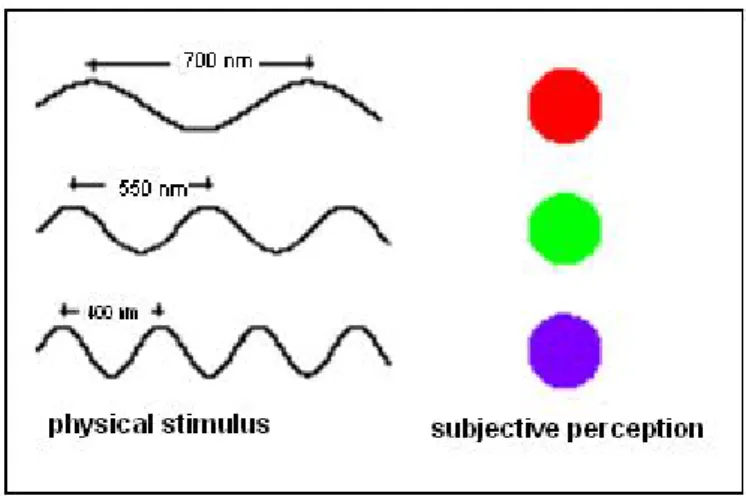
First, it is necessary to introduce the color concept: the color is a visual perception caused by a

physical stimulus, the light, which directly or indirectly, affects the eye, (particularly the retina), arrive through the optic nerve arrive to the brain, where the sensation of color is created.

The light is composed of monochromatic electromagnetic radiation of different wavelengths included between 400 nm (ultraviolet) and 700 nm (infrared). Every single monochromatic radiation is perceived by the eye as a single color, as shown in the figure below.

Figure 3.1 The eye perceives each monochromatic radiation as a color.

It is possible to build the color spectrum shown in Figure 3.2, putting below all visible monochromatic radiations with their wavelength, and the respective perceived colors:

Figure 3.2 The spectrum of colors. .

(18)

- 13 -

In this spectrum, however, some color like white, black, gray and many other are missing. The reason of this fact is that, normally, in nature, the lights are a mixture of different monochromatic radiations which are perceived by the eye do not individually but as a “total” color. These colors are called "non-spectral" and the white of sunlight, which contains all visible wavelengths, is one example.

It is important, therefore, to distinguish between two different worlds: one physical, objectively describable and measurable with precision and another one perceptual where subjective variables come into play.

Normally the way in which we see a color is influenced by several factors, which can be grouped into three main categories: psychological / emotional, physiological and environmental.

The psychological / emotional affects are related to how a person interprets a certain color. The blue and green colors, for example, are cold and have a relaxing effect; black and white are associated with the death and purity concept respectively.

These factors are very important in all those activities defined as "color-critical", like, for example, the advertising that tries to influence people taking advantage, too, the feelings aroused by the colors used in ads or products.

The physiological factors concern, however, the manner in which the receptors present in our eyes (cones) produce signals that determine the sensations of colors. The behavior of these "sensors" varies from individual to individual, and sometimes malfunctions that lead to the inability to distinguish certain colors can exist.

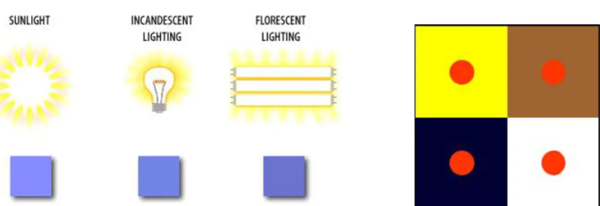
The environmental factors are related to light and colors of the place in which a color is seen. The figure below shows how the color perception can be strongly affected by the type of ambient light (on the left) and by the colors around it (on the right). This phenomenon is called "Achromatic Simultaneous Contrast": the red dots, although they are identical, seem to have different brightness.

(19)

- 14 -

At this point, it is questionable what laws govern the color perception. The first to give an answer to this question was Isaac Newton (1642-1727), who in 1666 drew the diagram shown below, which he regarded as approximate.

Figure 3.4 The Newton diagram.

Newton has decided to combine the extremes of the color spectrum, resulting in a circle. The spectral colors, in this model, are on the circle, while those not spectral are inside. The white is placed at the centre. A third dimension that goes perpendicular to the plane is implied: the brightness.

3.2. The CIE colorimetric model

The CIE colorimetric model, proposed by Commission Internationale de l'Eclairage in 1931, represents all and only the colors that the human eye can see and it is illustrated by the following figure.

Figure 3.5 The CIE 1931 chromaticity diagram.

This chromaticity diagram, which is that of Newton, modified, updated and standardized, is two-dimensional: the white is in the centre and the saturated color of the light spectrum are along the

(20)

- 15 -

curve portion of the perimeter: in clockwise direction, red, yellow, green, blue, purple. The central colors are unsaturated (white is the most unsaturated) and peripheral colors are saturated. The diagram represents the colors (around the perimeter) and saturation (from the perimeter toward the centre).

Each color is represented by a point inside the horseshoe area. The entire area is included in a system of x, y Cartesian coordinates as shown below.

Figure 3.6 x, y coordinates in the CIE 1931 color space.

Both x and y coordinates take values from 0 to 1. At each color corresponds a pair of x, y coordinates, but not at all of the pairs of coordinates in the range corresponds a color. For example, there is a certain red defined by the coordinates x = 0.6 and y = 0.3, the color of (0.4,0.2) coordinates is a lilac while the (0.1, 0.6) color is a green.

Note that in the diagram the two x and y coordinates are denoted by lowercase, since in colorimetry X and Y case have another meaning.

Up to this point the brightness of the colors is not considered; it can be introduced by adding a third dimension to the just seen diagram.

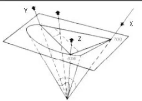
In fact, the CIE 1931 chromaticity diagram is only a "slice" of a more complete space, the CIE 1931 color space to which the coordinates XYZ are assigned. This space has the form shown in the image below, where the chromaticity diagram is individuated (in a form slightly different from the one considered here).

(21)

- 16 -

Figure 3.7 The XYZ space. Its projection on a plane is an xy chromaticity diagram.

The Y coordinate of the XYZ space, for how this space is constructed, expresses the brightness of considered color.

The relations to switch from three-dimensional XYZ coordinates to xy coordinates are: x = X / (X + Y + Z), y = Y / (X + Y + Z)

It is also possible to consider another coordinate system: the space xyY, obtained by adding the third dimension to the xy diagram, ie, the Y coordinate.

The two systems x,y,Y and X,Y,Z constitute two different coordinate systems for the CIE 1931 chromaticity diagram; they are mathematically linked to each other, and if you know the coordinates of a color given by x,y,Y system, it is possible to know her coordinates given by X,Y,Z system and vice versa.

The formulas to switch from xyY to XYZ, with a Y fixed are: X = xY / y, Z = (1-x-y) Y / y

The spaces x,y,Y and X,Y,Z allow, therefore, to express the same colors in the same CIE 1931 chromaticity diagram with two different but connected coordinate systems. You choose one of the two systems according of the use and convenience of data processing.

Before introducing an important property of the CIE 1931 diagram, we see at a glance how colors are produced with the additive mixture.

There are at least 3 types of additive mixture: • Space;

• temporal average; • spatial average.

The additive mixture space is obtained when more lights, which produce different sensations regardless of color, are superimposed. In this case, they produce a new color sensation. For example, if two lights that, which produce the sensation of red and green independently, are overlapped, the produced sensation will be of yellow (Fig. 3.8).

(22)

- 17 -

Figure 3.8 The additive mixture Space.

With the additive mixture in the time average, the different radiations strike the eye at different times, but so close together (at least 50, 60 times per second) that the eye draws a single media sensation.

For example, if a wheel with red and green colored areas is spun rapidly, a sensation of a brown color (dark yellow) will be produced..

The additive mixture in the spatial averaging is the most common case in practice. For example, monitors and televisions are based on additive synthesis, because the dots of R, G and B phosphors are neighbors and are so small as to be indistinguishable; in the eye and blend into a single point on the retina.

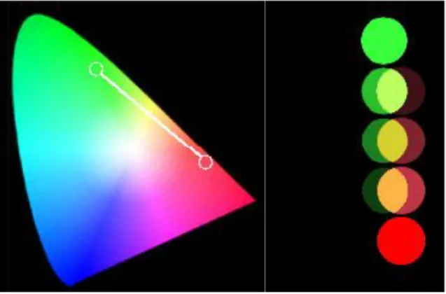
An important property of the CIE 1931 system is illustrated. If you mix two colors in additive synthesis, a third color is obtained; a series of other colors can be obtained by varying the proportions of the first two colors.

For example, starting with a green and a red (right below) and mixing them in different proportions various colors including yellow are obtained. How these colors are arranged on the CIE 1931 chromaticity diagram? Newton concluded that the different resulting colors are on a straight segment that joins the two initial colors, and this result is also valid in the CIE 1931 (left below).

(23)

- 18 -

This is an important property of the CIE 1931 chromaticity diagram: additively mixing two colors, represented by two points on the diagram, it is possible to get all colors that are on the segment connecting the two points, by varying the proportions of the two initial colors.

In particular, fixed two colors at certain luminosity, the brightness in their additive mixtures are added and the resulting color is in the barycentre of the brightness. If the brightness are the same, the color is in the centre.

So, if you mix a green and a red both with a brightness equal to 1, a yellow with brightness equal to 2, will get and this yellow will be half way between green and red.

By additively mixing three colors, represented by three points on the diagram, all the colors that are inside the triangle of which three points are the vertices, will get.

Figure 3.10 The synthesis of three additive colors.

The majority of the colors, even if not all, can be generated placingthe three vertices equally spaced on the perimeter. This is the trichrome principle.

3.3. Chromatic Adaptation

The human visual system optimizes its response to the particular viewing conditions with a dynamic mechanism called adaptation; it ca be of two types: color and luminance.

The adaptation to the luminance consists in a variation of the visual sensitivity when the light level increases or decreases. To realize this behavior, just pass by a very bright in a dark room: you can not initially see anything, then the eye begins to gradually adapt to darkness and see better.

The chromatic adaptation occurs, however, when an object under different lighting types (eg natural light first, then a light bulb) is observed: if the observer has had sufficient time to allow the eyes to adjust to new light source, the object retains its appearance under both illuminations.

(24)

- 19 -

The chromatic adaptation is, therefore, the ability of our visual system to discard the illumination color and to preserve in an approximate manner the appearance of an object.

Now consider a piece of paper and two light sources represented by the following coordinates in the xy chromaticity diagram: D65 (0.3127,0.3290) and D50 (0.3457,0.3585) (these are two of the standard light sources of the "D" series, introduced in 1963 by CIE. The standardization of the light sources has been carried out to allow to define the artificial light sources used in the industry to evaluate the colors).

• Scenario 1: the piece of paper illuminated by D65, has by definition the chromaticity coordinates of D65. An eye adapted to D65 sees by definition this white paper.

• Scenario 2: if the same piece of paper is illuminated with D50 its chromatic coordinates will become those of D50. Thus, for a measuring instrument, the piece of paper has changed color. But to the eye adapted to D50, the paper will appear as white as before.

• Scenario 3: if the piece of paper is modified so that the instrument sees it the same as before, the adapted eye will see a different color.

This is because measurement systems that rely on colorimetry does not take into account (or do not have the) the ability to adapt to the enlightening of the human eye.

The various tools to capture and display images must, therefore, deal with different types of light sources, since these can change switching from one device to a different one. A monitor, for example, may have a white point lies between the D50 and D93coordinates, and, therefore, two different displays may represent the white with different coordinates in the xy chromaticity diagram (ie they have two different points of the white).

To create the appearance of a color image, all these systems have to apply a transformation to the input color (captured with some enlightening) to convert it in the output color .

And this is the purpose of transformations for chromatic adaptation. Applying these transformations to the X 'Y' Z values of a color under a given illuminant, we can calculate a new set of three X "Y" Z "coordinates related to a different illuminant.

All transformations use the same basic methodology:

1. transform the XYZ coordinates in the tristimulus values of the cone responses; 2. change those responses;

3. reprocess these values in XYZ.

The most commonly used transformations are: • XYZ linear scaling;

(25)

- 20 -

• Bradford transformation (Lam and Rigg, Ph.D. thesis, University of Bradford, 1985).

3.4. The LAB color space

Another color space that, such as the XYZ space, representes all the colors that the human eye can see, is the CIELAB space.

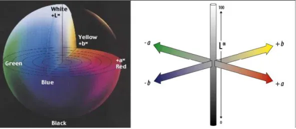
As shown in Figure 3.11, the LAB model is spherical and represents the colors through three components: the L axis is the brightness that varies from 0 (black) to 100 (white); the a and b axes spectively define the ranges of colors from red to green and from yellow to blue.

Figure 3.11 The CIELAB color space.

Note how the brightness is "separate from the color"; it means that it does not depend on the values assumed from the a and b channels. Instead, as we shall see, in the RGB and CMY spaces, the brightness is related to the values of the three channels.

It is possible to switch between the different XYZ, and LAB xyY coordinate systems using appropriate mathematical formulas, without loss of information.

(26)

- 21 -

3.5. RGB and CMYK color models

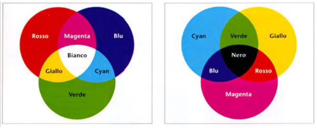
The RGB color space is the natural "language" of color description used by electronic devices such as monitors, scanners and digital cameras, that reproduce colors by transmitting or absorbing light rather than reflect it. The colors observed on computer monitors, for example, appear when the electron beams strike the red, green and blue phosphors of the screen causing the emission of different combinations of light.

The RGB color space is called additive because colors are generated by adding colored light to other colored light. The secondary colors are brighther than red, green and blue primary colors that are used to create them. In RGB mode the maximum intensity of the primary colors produces the white. A combination of identical amounts of red, green and blue produces neutral gray tones; dark grey tones are generated using low values of dark gray, while lighter tones are created with higher values. The figure below left shows the RGB space.

Figure 3.12 Color models RGB and CMY.

The right part of Figure 3.12, instead, represents the color space complementary to the RGB, obtained by subtracting the primary R, G and B colors from white light. This type of color representation is called CMY mode and it is the one used by the printing industry and, in general, by the printing devices. As can be clearly seen in the figure, the CMY space is subtractive: while in the RGB space the light is added to another light resulting in brighter colors, in CMY mode the light is subtracted, producing darker colors.

For completeness, it should be stressed that the RGB and CMY spaces are complementary to each other only in theoretical line. By combining, in fact, equal amounts of cyan, magenta and yellow neutral grays should form and combining the maximum quantity you should get the black (the opposite of white in the RGB model). This is true on monitors, but, in print, a muddly brown is obtained instead of the black and this phenomenon is caused by impurities in the pigments of the

(27)

- 22 -

inks. For this reason it is necessary to add another color, the black (denoted K by key color ) that allows for deeper blacks and shadows with definite sharper. Obviously, the addition of a fourth color unbalances the equation for the direct conversion from RGB to CMYK making more complicated the correspondence between these two color spaces.

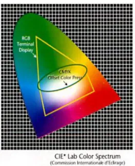
One last thing to remember is that the RGB and CMYK color spaces are device-dependent and, therefore, the colors generated by a device may differ from those played by another. All this does not happen, however, with the colors identified by CIE XYZ and LAB models that, such as visual perception, are not tied to specific devices and are much more numerous than those represented in RGB and CMYK :this is the reason for whicht he programs for the digital color management exploit the CIE as a base to convert the colors in sure way, then considering the limitations of the range of input and final output devices.

The diagram below shows the relationship between the viewed color mode.

(28)

- 23 -

4. State of the art

4.1 JPEG

In the late '80s the engineers of the ISO / ITU decided to form an international research team to create a new standard format of photographs recordings which allowed a strong reduction of the space occupied in memory at the expense of a more or less marked but always acceptable quality degradation. Thus the Joint Picture Expert Group was born and in 1992 released the popular JPEG compression format, which takes its name from this group.

Before the JPEG advent, BMP, TIFF, GIF, TARGA, the IFF and the other format images were typically used. All these formats, however, were marked by the loss-less compression, that is, without any loss of information and therefore were unable to obtain satisfactory compression ratios. For example, the BMP not apply any compression and simply provides an array of 'words', each of which defines the color of the corresponding pixel (eg using 8,16 or 24 bit); the TIFF instead apply entropic techniques such as RLE or Huffman compression (or LZW) to reduce the image size. These techniques have some effectiveness especially in those cases where not all the image surface contains relevant information; this occurs for example in images with large areas of a single color but it is difficult to obtain satisfactory compressions with photographic images. Finally, the GIF format was not suited to handle photographic images because it is limited to the use of a maximum of 256 colors. All of these methods, typically, did not allow to reduce the size more than a 2 factor. The JPEG was a decisive forward step in image compression, and quickly established itself especially with the birth of the WWW that necessarily needed a very simple format for transmission over the Internet. Note that an image of 500 x 500 pixels in full-color occupies something like 750KB in uncompressed format, while JPEG allows to reduce its size by a 20-30 (or even more) factor, depending on the level of chosen detail, that is the number of details discarded during the compression phase. The utility is obvious: the original image is changed from 750KB to only 30KB; it is then easily storable on magnetic supports and transferable over the Internet even using an ordinary modem.

(29)

- 24 -

How JPEG works

JPEG is a flexible standard that defines a set of possible processes to be performed on images, processes that can also be skipped. A guideline for compression and especially a rigid specifications for decompression is given. In practice, it is not specify how to do compression, but only the rules that must be observed by the compressed data, in order to obtain a correct decompression.

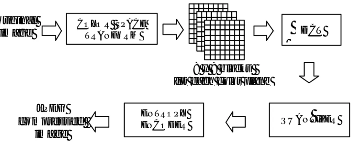
In any case there is a more or less standard process, which is illustrated in this image:

Figure 4.1JPEG encoder architecture.

a) Conversion of color space (optional)

The original image is converted from RGB to YIQ (or YUV) color space. The YUV format consists of 3 color planes: the luminance (Y) and two chrominance components (U and V). This separation, though not strictly necessary, allows for better compression. In fact, exploiting a phenomenon known in the video, you can reduce the size of the YUV image with a slight reduction in quality by applying a downsampling (decimation) of the chromatic components and keeping intact the luminance information.

The reduction is typically done by making the average, two by two, between adjacent pixels of the U and V planes; in practice the horizontal resolution of these plans is halved. In theory it is possible also to halve the vertical resolution (eg in MPEG1) but it is not a practice typically used in JPEG. In the first case we speak of 4:2:2 encoding and of 4:1:1 in the second case (at each block of 2x2 pixels in tY correspond 2x1 blocks in the first case and of a single pixel in the second case). Already this lossy arrangement (ie, with loss of information) allows a reduction of 30% and 50% respectively.

original

image COLOR SPACE _TRANFORM

JPEG compressed image ENTROPY ENCODER 8 x 8 blocks for each color plane

QUANTIZER D CT

(30)

- 25 -

If this step is skipped, the next phase will process the image in RGB instead of YUV.

b) Frequency Analysis (DCT)

The key development of JPEG is certainly the DCT (Discrete Cosine Transform) in its two-dimensional (2D) version. The DCT is a transform which in general converts the signal from the time to the frequency domain. This is a version in the real range of the FFT which is instead in the complex domain. The resulting coefficients represent the amplitudes of those harmonic signals (cosine) that added together reconstruct the signal.

JPEG uses the two-dimensional version of the DCT and in this case there is no mention of time and frequency but only of space and spatial frequencies. In order to be processed, the image is divided into color planes (three color planes RGB or YUV depending on the stage before) and within each plane it is again divided into blocks of 8x8 pixels.

The block of 8x8 pixels in the domain of the 'space' is transformed into a block of 8x8 coefficients in the spatial frequency domain. In this block, the coefficients in the upper left represent the low spatial frequencies while those gradually in the lower right, represent the high spatial frequencies, that are the image details. In particular, the first coefficient of the transformed block represents the average of the values of the original 8x8 block (also called DC component).

The mathematical formula of 2D DCT is shown below:

                         

_

    ) 1 2 ( 2 ) 1 2 ( 2 cos ) , ( 4 ) , ( 2 2 1 0 1 1 1 0 2 1 2 1 j N k i N k j i A k k B N j N i  

The original image is large N1 x N2 pixels; A (i, j) is the intensity of the pixel at i,j position; B (k1, k2) is the resulting coefficient. Typically, A is a number of 8 bits, and in output will have variable values between -1024 and 1023.

c) Quantization

The deletion of less important visual information occurs in this phase. This is accomplished by multiplying an 8x8 coefficients matrix in the frequency domain for a 'quantization table'. The table

(31)

- 26 -

contains values between 0 and 1, the lowest are located in correspondence of the high frequencies while the higher ones in correspondence of the low frequencies.

The values thus obtained are rounded to the nearest integer; in this way the least significant coefficients tend to zero while the coefficients related to the information contributions most important remain. High-frequency values are often rounded to 0, since they are already small. The result is the concentration of a few coefficients different from 0 at the top left and 0 all the others. When in a JPEG file you choose the compression factor, indeed you choose a scale factor on the values of 'quantization table'. The number of coefficients that are set to zero grows in proportion to the decrease of their values, with a consequent reduction in the number of significant coefficients. This process, of course, erases information more and more important and leads to a progressive deterioration of the compressed image quality.

d) Entropy coding

Once removed the less important details thanks to the DCT and quantization, it is necessary to adopt a series of entropic techniques to reduce the amount of memory required to transmit the remaining significant information.

It is important to separate the continuous component (indicated as DC in the figure) from the variable component (indicated with AC), among the remaining coefficients. The two types of values will be treated separately.

Figure 4.2 Zig-Zag sequence.

d1) Zig-Zag reading

The AC component is scanned by a Zig-Zag reading. Looking at the figure above it is clear what it means. The Zig Zag reading makes as much as possible adjacent the coefficients equal to 0 and allows an optimal data representation using Run Length Encoding.

(32)

- 27 -

d2) RLE on the variable component (AC)

Run Length Encode (RLE) is a simple compression technique applied to the AC components: the 1x64 vector resulting from Zig-Zag reading contains a lot of zero in sequence. For this reason the vector is represented by pairs (skip, value), where skip is the number of values equal to zero and

value is the subsequent value different to zero. The pair (0.0) is considered as a signal of end

sequence.

d3) DPCM on DC component

A technique called DPCM is instead applied on the DC value of each block. In practice it is possible to encode the DC component of a block as the difference compared to the value of the previous block because, generally, a statistical relationship in images among the DC components of adjacent blocks exists. This trick allows a further reduction of the space occupied by the data.

d4) Huffman compression

The classic variable code length coding is the last entropy coding applied to the data. The data is divided into 'words' (strings of bits); the statistical frequency of each word is analyzed and each word is recoded with a variable length code according to frequency of appearance. A short code for the words that appear frequently and progressively longer codes to less frequent ones. Altogether the number of bits needed to represent the data is reduced consistently.

Decompression

JPEG is a symmetrical code for its own nature and then the processing required for decompression is the exact inverse of that required for the compression.

The Huffman decompression is applied on compressed data; the resulting data are used for the reconstruction, block after block, of DC and AC components, then the coefficients are multiplied by an inverse quantization table. The resulting 8x8 block is subjected to an inverse DCT and at this point, depending on the settings of the file, the RGB image has already obtained, or you must do the YUV -> RGB conversion.

(33)

- 28 -

Conclusion

JPEG is a standard quite simple in its essence and yet the importance it has assumed in computing has been and is still really huge. Think of how many JPEG images are downloaded via the Internet every day, think of how many images are stored in digital cameras or digital video codec to be processed (many codec use the basics of JPEG compression to compress images sequences that form the video). All that would not have been possible without the commitment of the Joint Picture Expert Group. But as with many other technologies the JPEG is approaching to retirement age. Indeed, the new JPEG2000 standard promises better performance in compression, higher quality and more features in the security.

(34)

- 29 -

4.2 JPEG 2000

In the previous section we discussed one of the most popular and disseminated to the world compression formats, the JPEG. The mathematical principles which are the basis of the famous image compression format have been described.

JPEG is universally accepted as the standard 'de facto' in the field of lossy compression of images. Recall also that the basic mathematical tool in the JPEG (DCT) is used both in video compression of movies (MPEG, DiVX) and in audio compression (MP3).

However, in December 2000, the ISO / ITU has completed the standardization process and adoption of the new compression image algorithm, JPEG2000, which probably will become the successor to JPEG.

But how JPEG 2000 exactly works? What are the main differences from the older brother JPEG? Will JPEG 2000 definitively replace JPEG or will the glorious predecessor still have space?

How JPEG 2000 works

The differences compared to JPEG are numerous, indeed we can say that the two formats differ in almost all areas. The main evolution is certainly represented by the change of the basic mathematical tool at the base of the compression algorithm. While, as we explained previously, JPEG uses DCT (Discrete Cosine Transform) and operates on 8x8 blocks of pixels, JPEG 2000 uses the DWT (Discrete Wavelet Transform) and essentially operates on the entire image.

The word wavelet refers to the particular decomposition that is made of the image information. If the DCT decomposes the image into harmonic components (in practice is a frequency analysis) and block by block, the DWT breaks down the entire image into subbands a cascade. By adopting this approach and extending the analysis to the entire image, it eliminates the main drawback of JPEG: the excessive “tiling” that occurs with increasing the compression factor. This type of filtering (that will analyze in detail later) is obtained by the convolution of the image with the particular FIR filters, that remember 'small waves' for their structures.

(35)

- 30 -

- Support for different color spaces and modes (two-tone images, in grayscale, at 256 color, at millions of colors, in RGB standard, PhotoYCC, CIELAB, CMYK).

- Support for different compression schemes, adapted as needed.

- Open standard for subsequent implementations related to the emergence of new needs.

- Support for the inclusion of an unlimited amount of metadata in the space of the file header, used to provide private information or to interact with software applications (drive, for example, the browser to download appropriate plug-in from Internet).

- State of the art for the destructive and non-destructive images compression, with a saving of space at the same quality, compared to the JPEG standard, which starts from a +20-30%.

- Support for files larger than 64k x 64k pixels, or greater than 4 GB.

- Support for the data transmission in disturbed environments, for example through the mobile radio.

- Quality scalability (signal / noise ratio or SNR) and multi-resolution.

- Support for ROI (Region Of Interest) encoding, ie of areas considered most important and therefore saved with a greater resolution than that used for the rest of the image.

- Native support to the Watermarking or branding for the recovery of royalties.

Introduction to the Discrete Wavelet Transform

JPEG2000 uses the DWT (wavelet) transform in the main compression stage. The Wavelet transform decomposes gradually the original image in sub-band representations at multi-resolution. To understand how it works first consider the one-dimensional case.

A certain X signal is first split into two parts by passing it through a high pass filter (AH) and a low pass filter (AL). The two signals thus obtained are decimated by 2 (ie a sample is taken every 2) giving rise to two subbands XH and XL. If initially we had an X signal of N samples, now we have two signals XH and XL each consisting of N/2 samples. Generally they are the first order coefficients of the wavelet transform; XH is also called detail..

If the filters used respect certain characteristics, the process is reversible and it is possible to extract the original signal from the two components interpolating the coefficients and by passing them through appropriate filters. The low-frequency sub-band that typically contains the most important part of the signal, can be further decomposed a cascade as shown in the figure:

(36)

- 31 -

Figure 4.3 Decomposition of low-frequency sub-band.

In the two-dimensional case of an image, the signal (the image) is decomposed into sub-bands through three filters: a horizontal pass filter, a vertical pass filter and a diagonal high-pass. The resulting images are decimated both horizontally and vertically to form three groups of

detail coefficients (HL, HH, LH). The original image is also scaled of a 2 factor on X and Y and forms the LL sub-band in low frequency. This particular sub-band is then and repeatedly broken down at successive levels of decomposition (see image).

Figure 4.4 JPEG 2000 decomposition levels.

This type of representation with the use of DWT has many advantages that will see later.

JPEG 2000 in detail

Figure 4.5 JPEG 2000 encoder architecture.

original

image COLOR SPACE TRANFORM

JPEG2000 compressed image QUANTIZER ENTROPY CODER (EBCOT) () TILING DWT LEVEL OFFSET RATE CONTROL BIT STREAM ORGANIZATION

(37)

- 32 -

The JPEG2000 format expects several image processing steps; below we will explain the fundamental algorithms without going too deeply into mathematical issues and the numerous exceptions provided by the algorithm.

a) Pre-processing

The original image is first divided into non-overlapping tiles of equal size. Each tile is separately compressed and the compression parameters can be different from tile to tile.

The unsigned values that describe the pixels are properly shifted by a constant factor in order to be centred in 0. In addition, each tile is separated into color channels. Two basic color coding were defined in JPEG 2000, one reversible for lossless compression and the other one irreversible for lossy type and perfectly analogous to the conversion from RGB to YCbCr used in JPEG.

It is also possible to compress images in GrayScale and at levels.

b) DWT

The DWT operates over the whole image and causes a subsequent breakdown in sub-bands, each which treatable by importance taking in human vision. In the following images we can see the various levels of decomposition.

Figure 4.6 First DWT decomposition level.

At the first level, the original image was split into 4 sub-images (each with a quarter resolution of the original) that represent the details in high frequency and the content in low frequency.

(38)

- 33 -

Figure 4.7 Second DWT decomposition level.

The second level of decomposition operates on low frequency content generated by the first level. Other detail subbands and a new low-frequency subband are generated.

Figure 4.8 Third DWT decomposition level.

The process proceeds to successive levels by generating more and more detail subbands. The details generated at successive levels of decomposition are more important for the perceptual purposes of those generated in the early stages.

(39)

- 34 -

Figure 4.9 Resolution levels.

The filters used for the decomposition into sub-bands are called bi-orthogonal filters for their mathematical characteristics. Here are some examples of finite impulse response (FIR) filters used for the extraction of sub-bands; their characteristic gives the name to the wavelet encoding.

Figure 4.10 FIR filters.

c) Quantization

The behaviour of the human eye compared to the spatial frequency of the images may be determined by the response to harmonic images. It is possible to draw a function of the sensitivity of the human eye to the contrast changes. This sensitivity is maximal for images that are 5 harmonious cycles for viewing corner, while vanishes almost completely for images with 50 cycles for corner.

(40)

- 35 -

This feature allows us to define the appropriate quantization values for the relevant sub-bands. It is clear that the first sub-bands of detail can be quantized with accuracy much smaller than in later ones since the human eye can not perceive low entity changes at high spatial frequencies. The exponential decreasing shape of the curve also explains the reason of the decimation which is performed at each iteration.

Figure 4.11 Contrast sensitivity curve.

d) Entropy coding

The bits uniformly quantized in the quantization stage are handled in bit-plane. This aggregation of data results in a substantial inefficiency of the Huffman entropy coding ( referred to JPEG case). To ensure efficient entropy coding is necessary to merge pattern of bits in configurations at high probability.

The "arithmetic coding" provide excellent performance in these cases and allow to deviate from the theoretical peak performance of just 5-10%. The arithmetic codes used in the JPEG2000 are also adaptive and estimate the symbols probability based on adjacent pixels values adapting to the image content.

The entropy coding takes place for the code-block (eg 8x8 pixels). The bit planes of each block are examined in succession from MSB (Most Significant Bit) to LSB (Least Significant Bit).

(41)

- 36 -

This approach allows to decode the image, bit plane by bit plane, in order to give the decoding scalable in terms of signal to noise ratio (SNR).

e) Generation of the final bit-stream

In the previous step a bit-stream for each code-block was generated; in this phase the bit-stream is organized to be able to easily handle the scalability in quality (SNR) and resolution. This aim is achieved by packing the data for bitplane and then for decomposition levels. In the decompression phase, it is possible to use only a certain number of bitplanes (from the MSB onward) depending of the desired quality. If a certain resolution is required, it is only necessary the treatment of subbands of higher order.

The two approaches can be combined. This feature of scalability and flexibility of the JPEG 2000 algorithm is one of the most interesting. The application servers will be able to provide services based on JPEG2000 managing the resolution and quality according to the application characteristics and the available bandwidth. JPEG 2000 will be the first step toward new video compression techniques in which we will have a single file to satisfy the most stringent requirements in terms of resolution, quality and, ultimately, the request band.

The final structure is not simple at all and then you just know that it is designed not only for scalability but also to satisfy two other interesting requirements: the management of ROI (Region Of Interest) and error robustness.

The ROI coding is the ability to encode different parts of the image with different parameters and different qualities. The choices can be made both in the compression and in content delivery phase and in this case managed from a server according to the user needs.

JPEG 2000 also provides strategies for using the format in disturbed channels with minimal loss of functionality. Unlike JPEG in which the loss of data determines the irremediable corruption of video blocks, the robust JPEG2000 encoding allows to ensure high standards of quality even on noisy channels. It will be particularly appreciated on cellular systems as well as for streaming systems in broadcast where the loss of packets is, in this way, tolerable.

JPEG XR scalable coding for remote image browsing applications

Università degli Studi di Cagliari

DOTTORATO DI RICERCA

IN INGEGNERIA ELETTRONICA ED INFORMATICA

Ciclo XXIII

JPEG XR SCALABLE CODING FOR REMOTE IMAGE BROWSING

APPLICATIONS

ING-INF/03 (Telecomunicazioni)

Presentata da:

Bernardetta Saba

Coordinatore Dottorato

Prof. Alessandro Giua

Tutor/Relatore

Prof. Daniele Giusto

To Roberto

and my family

Contents

1. Introduction

2. Image compression

2.1 The need to compress images

2.2 Compression techniques

2.3 Lossless compression

The Huffman algorithm

The RLE (Run Level Encode) algorithm

The LZW (Lempel-Ziv-Welch) algorithm

2.4 Lossy compression

2.5 Relative redundancy and compression ratio

2.6 Reversibility

2.7 Fidelity

2.8 The efficiency of the coefficient

3. Color management

3.1.

The color

3.2.

The CIE colorimetric model

3.3.

Chromatic Adaptation

3.4.

The LAB color space

3.5.

RGB and CMYK color models

4. State of the art

4.1 JPEG

How JPEG works

a) Conversion of color space (optional)

b) Frequency Analysis (DCT)





c) Quantization

d) Entropy coding

d1) Zig-Zag reading

d2) RLE on the variable component (AC)

d3) DPCM on DC component

d4) Huffman compression

Decompression

Conclusion

4.2 JPEG 2000

How JPEG 2000 works

Introduction to the Discrete Wavelet Transform

JPEG 2000 in detail

a) Pre-processing

b) DWT

c) Quantization

d) Entropy coding

e) Generation of the final bit-stream

_

_