On the monotonicity of scalar curvature in classical and quantum information geometry

(1)

On the monotonicity of scalar curvature in classical

and quantum information geometry

Paolo Gibiliscoa兲

Dipartimento di Studi Economico-Finanziari e Metodi Quantitativi, Facoltà di Economia, Università di Roma “Tor Vergata,” Via Columbia 2, Rome 00133, Italy and Centro “Vito Volterra,” Università di Roma “Tor Vergata,” Via Columbia 2, Rome 00133, Italy Tommaso Isolab兲

Dipartimento di Matematica, Università di Roma “Tor Vergata,” Via della Ricerca Scientifica, 00133 Rome, Italy

共Received 30 June 2004; accepted 5 October 2004; published online 18 January 2005兲 We study the monotonicity under mixing of the scalar curvature for the ␣-geometries on the simplex of probability vectors. From the results obtained and from numerical data, we are led to some conjectures about quantum␣-geometries and Wigner–Yanase–Dyson information. Finally, we show that this last conjecture implies the truth of the Petz conjecture about the monotonicity of the scalar curva-ture of the Bogoliubov–Kubo–Mori monotone metric. © 2005 American Institute of Physics. 关DOI: 10.1063/1.1834693兴

I. INTRODUCTION

The Bogoliubov–Kubo–Mori共BKM兲 metric is a distinguished element among the monotone metrics which are the quantum analog of Fisher information on the quantum state space.35,36In a definite sense BKM metric is the geometry on the state space that is related to von Neumann entropy共say, Umegaki relative entropy兲. Other well-known elements of this family are the right logarithmic derivative共RLD兲 metric, the symmetric logarithmic derivative 共SLD or Bures兲 metric, and the Wigner–Yanase–Dyson共WYD兲 metrics. In Ref. 34 Petz made a conjecture on the scalar curvature of the BKM metric. Many arguments and numerical calculations suggest that the con-jecture is true; nevertheless, a complete proof is still missing共see Refs. 3, 4, 12, 24, and 32兲.

One can state this conjecture in the following way: the BKM scalar curvature is a quantitative measure of symmetry共like entropy兲, namely it is increasing under mixing. Let us emphasize that it is also possible to relate the conjecture to quantities with direct physical meaning. An equivalent formulation, still due to Petz,34 is that “…the scalar curvature is an increasing function of the temperature….” Moreover, the asymptotic relation between volume and curvature in Riemannian geometry and Jeffrey’s approach to priors in statistics induced Petz to interpret the scalar curvature as the average statistical uncertainty共that should increase under coarse graining; see Ref. 36兲.

The original motivations given by Petz for the conjecture rely on the truth of the 2⫻2 case and on some numerical results for the general case. Petz and Sudar observed in Ref. 38 that “…monotonicity of Kubo metric is not surprising because this result is a kind of reformulation of Lieb convexity theorem.30 However the monotonicity of the scalar curvature seems to be an inequality of new type 共provided the conjecture is really true兲….” A recent clear reference for Lieb’s result and related inequalities can be found in the paper by Ruskai.40

The goals of the present paper are the following.

共1兲 We want to look at “higher mathematics from an elementary point of view.” This means that we want to furnish an elementary motivation for the Petz conjecture. We do this by studying

a兲

Electronic-mail: gibilisco@voterra.mat.uniroma2.it b兲_{Electronic-mail: isola@mat.uniroma2.it}

46, 023501-1

(2)

the monotonicity of the curvature for␣-geometries in the plane. The results obtained in this case are very intuitive if one looks at the unit sphere of the Lp_{spaces. We conjecture that a} similar behavior occurs for␣-geometries in higher dimensions and in the noncommutative case, too.

共2兲 On the basis of the results of point 共1兲 we make a conjecture about the monotonicity of scalar curvature for the WYD metrics. Further, we show that, using a continuity argument, this WYD conjecture would imply the Petz conjecture as a limit case共Theorem 8.1兲.

共3兲 We review what is known about monotonicity of scalar curvature for quantum Fisher infor-mation. In particular, we emphasize a result on the Bures metric, attributed to Dittmann, according to which the scalar curvature, in this case, is neither increasing nor Schur-decreasing共see Sec. II for precise definitions兲. This implies that an example of a monotone metric for which the scalar curvature共or its opposite兲 is strictly increasing under mixing does not exist yet. Note that Andai共using an integral decomposition of Ref. 15兲 proved that also in the 2⫻2 case there exist monotone metrics whose scalar curvature is not monotone.3 Finally, let us note that, related to this area, there exist other interesting papers. Some authors have suggested that, when statistical mechanics is geometrized, then the scalar curvature should have important physical meaning共for example, it should be proportional to the inverse of the free energy; see Refs. 8, 9, 25–27, and 39兲.

II. MAJORIZATION AND SCHUR-INCREASING FUNCTIONS

For the content of this section we refer to Refs. 1, 5–7, and 31.

A. Commutative case

We shall denote byPnthe manifold of positive vectors ofRn_{, and by}_Pn1_傺Pn_{the submanifold}

of density vectors, namely Definition 2.1:

Pn1_{: =}

再

_␳_{苸 R}n_兩

兺

i

␳i= 1, ␳i⬎ 0

冎

.

We set e : =共1, ... ,1兲. The trace of a vector is Tr共v兲=兺i=1n vi. For an n⫻n real matrix, consider the following properties:

共I兲 tij艌0 i, j=1, ... ,n, 共II兲兺i=1n tij= 1 j = 1 , . . . , n, 共III兲兺j=1n _t ij= 1 i = 1 , . . . , n. Definition 2.2:

共a兲 T is said to be stochastic if (I),(II) hold;

共b兲 T is said to be doubly stochastic if (I),(II),(III) hold.

When T is seen as an operator T :Rn→Rn共by 共Tv兲j=兺i=1n tjivi兲, then the properties 共I兲,共II兲,共III兲 can be written as

共I兲⬘ 共positivity preserving兲 Tv艌0 if v艌0; 共II兲⬘ 共trace-preserving兲 Tr共Tv兲=Tr共v兲 ∀v苸Rn_; 共III兲⬘ 共unital兲 Te=e.

Let x苸Rnbe a vector. We define x↓ as a vector with the same components in a decreasing order so that

x₁↓艌 x₂↓艌 ¯ 艌 xn↓.

(3)

x₁↓艋 y₁↓,

x1↓+ x2↓艋 y1↓+ y2↓,

¯ ,

x₁↓+ ¯ + xn−1↓ 艋 y₁↓+ ¯ + yn−1↓ ,

x₁↓+ ¯ + xn↓= y₁↓+ ¯ + yn↓. For example, if 共␳1, . . . ,␳n兲 is a density vector then

冉

1 n, 1 n, . . . , 1 n

冊

Ɑ 共␳1, . . . ,␳n兲 Ɑ 共1,0, ... ,0,0兲.

The relation Ɑ is a preordering but not a partial ordering. If xⱭy and yⱭx then x=Ty for some permutation matrix T.

Theorem 2.1:

xⱭ y⇔x = Ty where T is doubly stochastic.

Definition 2.4 (see Ref. 31 pp. 14 and 54): A real-valued function f defined on a setA傺Rn_is said to be Schur-increasing onA if

xⱭ y on A⇒ f共x兲艌 f共y兲.

If, in addition, f共x兲⬎ f共y兲 whenever xⱭy but x is not a permutation of y, then f is said to be strictly Schur-increasing. Similarly f is said to be Schur-decreasing onA if

xⱭ y on A⇒f共x兲艋 f共y兲,

and f is strictly Schur-decreasing if strict inequality f共x兲⬍ f共y兲 holds when x is not a permutation of y.

Of course, f is Schur-increasing if and only if −f is Schur-decreasing.

Remark 2.1 (see Ref. 31, p. 54):A傺Rnis symmetric if x苸A⇒⌸x苸A for all permutations ⌸. A function f is symmetric on A if f共x兲= f共⌸x兲 for all permutations ⌸. Let D: =兵x兩x1艌¯

艌xn其. If f is symmetric on a symmetric set A and increasing on D艚A, then f is Schur-increasing onA.

Remark 2.2: Let us consider the following identification I :共0,␲/ 2兲→P₂1 defined by I共␪兲 : =共cos2␪, sin2␪兲. Evidently, if␪1,␪2艋␲/ 4, then

␪1艋␪2⇔I共␪1兲 Ɱ I共␪2兲.

Any function onP₂1can be seen as a function on共0,␲/ 2兲. By abuse of language we shall use the same symbols to denote the two functions. SinceP₂1is symmetric we have, because of Remark 2.1 Proposition 2.2: A symmetric function f onP₂1is Schur-increasing if and only if f is increas-ing as a function on共0,␲/ 4兲.

B. Noncommutative case

Let Mnbe the space of complex n⫻n matrices. We shall denote by Hn the real subspace of Hermitian matrices, byDnthe manifold of strictly positive elements of M_n, and byD_n1傺Dnthe submanifold of density matrices, namely

Definition 2.5:

Dn1

(4)

If A苸Mn, let␭共A兲 be the n-vector of its eigenvalues, arranged in any order with multiplicities counted. If A is Hermitian then␭共A兲 is a real n-vector. Let A,B be Hermitian.

Definition 2.6:

AⱭ B⇔␭共A兲 Ɑ ␭共B兲.

Definition 2.7: A linear map ⌽ on Mn is doubly stochastic if it is positive-preserving, trace-preserving, and unital.

Theorem 2.3:

AⱭ B⇔A =⌽共B兲,where ⌽ is doubly stochastic.

Definition 2.8: A real-valued function f defined on a setA傺Hnis said to be Schur-increasing onA if

AⱭ B⇒f共A兲艌 f共B兲. Similarly, f is said to be Schur-decreasing onA if

AⱭ B⇒f共A兲艋 f共B兲.

Of course, f is Schur-increasing if and only if −f is Schur-decreasing.

III. PULL-BACK OF DUALITY PAIRINGS

To make the paper self-contained, we recall some constructions from Ref. 18.

Let V , W be vector spaces overR 共or C兲. One can say that there is a duality pairing if there exists a separating bilinear form

具·, ·典:V ⫻ W → R. LetM,N,N˜ be differentiable manifolds.

Definition 3.1: Suppose we have a pair of immersions 共␸,␹兲, where ␸:M→N and ␹:M →N˜ , such that a duality pairing exists between T_␸共␳兲N and T_␹共␳兲N˜ for any␳苸M. Then, we may pull-back this pairing onM by defining

具u,v典_␳␸,␹_{: =}_具D

␳␸共u兲,D␳␹共u兲典, u,v 苸 T␳M.

The most elementary example is given by the case where N=N˜ is a Riemannian manifold, ␸=␹, and the duality pairing is just given by the Riemannian scalar product on T_␸共␳兲N 共this is the pull-back metric induced by the map␸兲.

A nontrivial example is the following. Let X be a uniformly convex Banach space such that the dual X˜ is uniformly convex. We denote by 具·,·典 the standard duality pairing between X and X˜. Let J : X→X˜ be the duality mapping, that is J is the differential of the map v→1₂储v储2_{. J}_{共v兲 is the}

unique element of the dual such that具v,J共v兲典=储v储2₌_{储J共v兲储}2_.

Definition 3.2: LetM be a manifold. If we have a map␸:M→X we can consider a dualized pull-back that is a bilinear form defined on the tangent space ofM by

具A,B典_␳␸: =具A,B典_␳␸,Jⴰ␸=具D_␳␸共A兲,D_␳共J ⴰ␸兲共B兲典.

Example 3.1: For X a Hilbert space, J is the identity, and this is again the definition of pull-back metric induced by the map␸.

In what follows, if p苸R\兵0其 then p˜ is defined by 共1/p兲+共1/p˜兲=1. If p=1 then p˜= +⬁. Example 3.2: Let 共X,F,␮兲 be a measure space. If f is a measurable function and p苸共1, +⬁兲 then 储f储p: =共兰兩f兩pd␮兲1/p. Set

(5)

Lp= Lp共X,F,␮兲 = 兵f is measurable and 储f储p⬍ ⬁其. Define Np _{as L}p_{with the norm}

储f储Np: =储f储p

p . Obviously N˜ 共the dual of Np p兲 can be identified with N˜p.

Now, suppose that␳⬎0 is measurable and 兰␳= 1, namely␳is a strictly positive density. Then, v = p␳1/p_{is an element of the unit sphere of N}p_{and it is easy to see that J}_{共v兲=p˜␳}1/p_{. The family of}

maps␳→p␳1/pis known as Amari embeddings.

Let X =兵1, ... ,n其 and let␮be the counting measure. In this case Npis justRnwith the norm 储·储p/ p.

Proposition 3.1: Consider the Amari embedding ␸:␳苸Pn1→p␳1/p苸Np for an arbitrary p 苸共1, +⬁兲. Then, the bilinear form

具A,B典␳␸: =具A,B典␳␸,Jⴰ␸=具D␳␸共A兲,D␳共J ⴰ␸兲共B兲典, A,B 苸 T␳Pn1, is just the Fisher information.

Proof:

具D_␳␸共A兲,D␳共J ⴰ␸兲共B兲典 =

冕

共␳共1/p兲−1A兲共␳共1/p兲−1B兲 =

冕

AB

␳ .

䊐 The above result can be stated in much greater generality using the machinery of Refs. 19 and 14.

IV. SCALAR CURVATURE OF␣-GEOMETRIES

The ␣-geometries are one of the fundamental objects of information geometry 共see Refs. 2 and 20兲. The study of the monotonicity of their curvatures does not appear in the literature as far as we know. In this section we start such an investigation.

A. The plane case

Definition 4.1: The ␣-geometry on P₂1 is the pull-back geometry induced by the map Ap共␳兲:P₂1→R2_{defined by}

Ap共␳兲: =

再

p␳

1/p_, _p_{苸 R \}

兵

₀

其

_,

log共␳兲, p =⬁, where p = 2 /共1−␣兲.

Definition 4.2: We denote by cp共␳兲 the curvature of the␣-geometry关with p=2/共1−␣兲兴 at the point␳苸P₂1.

Remark 4.1: For the curvature cp共·兲 there are two easy cases: —if p = 1 then cp共·兲=const=0;

—if p = 2 then cp共·兲=const=₂1.

Taking a look at the unit sphere ofR2_{with respect to the L}p_{-norm, one can easily understand} the following general result.

Theorem 4.1: For the function cp共·兲:P₂1→R one has the following properties:

—if p苸共1,2兲 then cp共·兲 is a strictly Schur-decreasing function; —if p苸共2, +⬁兴 then cp共·兲 is a strictly Schur-increasing function.

Proof: Let us first consider p苸共1,⬁兲. Then, the ␣-geometry, ␣=共p−2兲/p, on P₂1 is the geometry of the set

(6)

2

pcos

2_␽_{− 1}

冊

_.

Let us parametrize density vectors as共cos2␪, sin2␽兲. In this way the curvature of␣-geometry at the point␳, namely cp共␳兲, is

cp共␽兲: = 兩x

⬘

y

⬙

− x

⬙

y

⬘

兩 关共x

⬘

兲2₊_共y

_⬘

_兲2_兴3/2=

p − 1 p

共sin␽cos␽兲共2/p兲+2

关共sin␽共cos␽兲1/p_兲4₊_共共sin_␽兲1/p_cos_␽兲4_兴3/2

= p − 1 p

冉

1 2

冊

2关1−共2/p兲兴 · 共sin 2␽兲 2关1−共2/p兲兴关共cos␽兲4/p˜₊_共sin_␽兲4/p˜_兴3/2= Ap· gp共␽兲 fp共␽兲32 , where we set Ap: = p − 1 p

冉

1 2

冊

2关1−共2/p兲兴 , gp共␽兲: = 共sin 2␽兲2−共4/p兲, fp共␽兲: = 共cos␽兲4/p˜₊_共sin_␽兲4/p˜_.

We want to compute the monotonicity properties of cpwith respect to the preorderingⱭ. We have

g_p

⬘

共␽兲: = 4共sin 2␽兲1−共4/p兲_·_共cos_␽_{+ sin}_␽兲

冉

_{1 −}2

p

冊

共cos␽− sin␽兲; since 0⬍␽⬍␲/ 2, then

4共sin 2␽兲1−共4/p兲·共cos␽+ sin␽兲 ⬎ 0, and therefore g_p

⬘

共␽兲 ⬎ 0⇔

冉

⬘

共␽兲 ⬎ 0⇔共sin␽兲共2/p˜兲−1⬎ 共cos␽兲共2/p˜兲−1⇔sin␽⬍ cos␽⇔0⬍␽⬍␲ 4.

Therefore, for 0⬍␽⬍␲/ 4, g is decreasing, f is increasing, and 1 / f3/2_{is decreasing. This implies}

that

cp= Ap gp f_p3/2 is strictly decreasing for 0⬍␽⬍␲/ 4.

Case: 2⬍p⬍⬁.

This implies 1 −共2/p兲⬎0,共2/p˜兲−1⬎0, and therefore

g_p

⬘

共␽兲 ⬎ 0⇔cos␽⬎ sin␽⇔0⬍␽⬍␲ 4,

f_p

⬘

共␽兲 ⬎ 0⇔共sin␽兲共2/p˜兲−1⬎ 共cos␽兲共2/p˜兲−1⇔sin␽⬎ cos␽⇔␲ 4 ⬍␽⬍

␲ 2.

Therefore, for 0⬍␽⬍␲/ 4, g is increasing, f is decreasing, and 1 / f3/2_{is increasing. This implies}

that

cp= Ap gp f_p3/2 is strictly increasing for 0⬍␽⬍␲/ 4.

Case: p =⬁.

Use now the following parametrization:

x = 2 log共cos␪兲, y = 2 log共sin␪兲, for the curve ex_{+ e}y_{= 1.Then}

共␽兲 = 2 sin␽cos␽共cos␽+ sin␽兲共cos␽− sin␽兲, f_⬁

⬘

共␽兲 = 4 sin␽cos␽共cos␽+ sin␽兲共sin␽− cos␽兲. This implies

g_⬁

⬘

共␽兲 ⬎ 0⇔cos␽⬎ sin␽, f_⬁

⬘

共␽兲 ⬎ 0⇔sin␽⬎ cos␽.

We have the same situation of the case 2⬍p⬍⬁ and therefore the same conclusion.

This ends the proof. 䊐

Note that we have also

Proposition 4.2: For the function cp共·兲:P₂1→R one has the following properties: if p 苸共−⬁,0兲 then cp共·兲 is strictly Schur-increasing.

Proof: Since 1 −2 p⬎ 0, 2 p ˜ − 1⬎ 1 ⬎ 0, 0 ⬍ p˜ ⬍ 1,

we have the same situation of the case 2⬍p⬍⬁ in the preceding Theorem 4.1 and therefore the

same conclusion. 䊐

If p苸共0,1兲 then cp共·兲 can have an arbitrary behavior 共Schur-increasing, Schur-decreasing, neither of the two兲.

B. The general case

Definition 4.3: The ␣-geometry on Pn1 is the pull-back geometry induced by the map Ap共␳兲:Pn1→Rndefined by

Ap共␳兲: =

再

p␳

1/p_, _p_{苸 R \ 兵0其,}

log共␳兲, p =⬁, where p = 2 /共1−␣兲.

Definition 4.4: We denote by Scalp共␳兲 the scalar curvature of the ␣-geometry 关with p =共2/共1−␣兲兲兴 at the point␳苸Pn1.

Of course the cases p = 1共flat geometry兲 and p=2 共geometry of a 共n−1兲-dimensional sphere with radius 2兲 are easy to study. One has

—if p = 1 then Scalp共·兲=const=0;

(9)

Again taking a look at the unit sphere ofRn_{equipped with L}p_{-norm, one can easily understand} the following conjecture.

Conjecture 4.1: Suppose n⬎2. For the function Scalp共·兲:Pn1→R one has the following prop-erties:

—if p苸共1,2兲 then Scalp共·兲 is a strictly Schur-decreasing function; —if p苸共2, +⬁兴 then Scalp共·兲 is a strictly Schur-increasing function.

C. Non-commutative case

Definition 4.5: The ␣-geometry on Dn1 is the geometry induced by the pull-back of the map Ap共␳兲:Dn1→Mn defined by

Ap共␳兲: =

再

p␳

1/p_, _p_{苸 R \ 兵0其,}

log共␳兲, p =⬁, where p = 2 /共1−␣兲.

Since the commutativity or noncommutativity of the context will always be clear, we perform a little abuse of language in the following definition.

Definition 4.6: We denote by Scalp共␳兲 the scalar curvature of the ␣-geometry 关with p =共2/共1−␣兲兲兴 at the point␳苸Dn1.

Again, the case p = 1共flat geometry兲 is obvious. The case p=2 is known 共see Refs. 16 and 17 or Theorem 7.2 below兲, and we have

—if p = 1 then Scalp共·兲=const=0;

—if p = 2 then Scalp共·兲=const=1₄共n2− 1兲共n2− 2兲.

Motivated by the commutative plane case we formulate the following conjecture.

Conjecture 4.2: Suppose n艌2. For the function Scalp共·兲:Dn1→R one has the following prop-erties:

—if p苸共1,2兲 then Scalp共·兲 is a strictly Schur-decreasing function; —if p苸共2, +⬁兴 then Scalp共·兲 is a strictly Schur-increasing function.

V. MONOTONE METRICS AND THEIR SCALAR CURVATURES

A commutative Markov morphism T :Rn_→Rm_{is a stochastic map. A noncommutative} Mar-kov morphism is a linear map T : Mn→Mmthat is completely positive and trace-preserving共note that in the commutative case complete positivity is equivalent to positivity; see, for example, Ref. 41兲.

In the commutative case a monotone metric is a family of Riemannian metrics g =兵gn其 on 兵Pn1 其, n苸N such that gT共␳兲 m _{共TX,TX兲艋 g} ␳ n_共X,X兲

holds for every Markov morphism T :Rn→Rmand all␳苸Pn1 and X苸T_␳Pn.

In perfect analogy, a monotone metric in the noncommutative case is a family of Riemannian metrics g =兵gn其 on 兵Dn1其, n苸N such that

g_Tm_共␳兲共TX,TX兲艋 g_␳n共X,X兲

holds for every Markov morphism T : M_n→Mmand all␳苸D_n1and X苸T_␳D_n1.

Let us recall that a function f :共0,⬁兲→R is called an operator monotone if for any n苸N, any A, B苸Mnsuch that 0艋A艋B, the inequalities 0艋 f共A兲艋 f共B兲 hold. An operator monotone func-tion is said to be symmetric if f共x兲=xf共x−1兲 and normalized if f共1兲=1. In what follows, by operator monotone we mean normalized symmetric operator monotone. With each operator mono-tone function f one associates also the so-called Chentsov–Morotzova function

(10)

cf共x,y兲: = 1 y f

冉

x

y

冊

for x,y⬎ 0.

Define L_␳共A兲: =␳A, and R_␳共A兲: =A␳. Since L_␳, R_␳commute we may define c共L_␳, R_␳兲. Now, we can state the fundamental theorems about monotone metrics共uniqueness and classification are up to scalars兲.

Theorem 5.1 (Ref. 10): There exists a unique monotone metric on P_n1 given by the Fisher

information.

Theorem 5.2 (Ref. 35): There exists a bijective correspondence between monotone metrics on

Dn1_{and operator monotone functions given by the formula}

具A,B典_␳,f: = Tr共A · cf共L_␳,R_␳兲共B兲兲.

共z,y兲, h: = h1− 1 2h2+ 2h3− h4. 共5.1兲

The functions hihave no essential singularities if arguments coincide.

Note that 具A,B典_␳f: = Tr共A·cf共L_␳, R_␳兲共B兲兲 defines a Riemannian metric also over Dn 共Dn1 is a submanifold of codimension 1兲. Let Scalf共␳兲 be the scalar curvature of 共Dn,具·,·典_␳f兲 at ␳ and Scal_f1共␳兲 be the scalar curvature of 共Dn1,具·,·典_␳f兲.

Theorem 5.3 (Ref. 12): Let␴共␳兲 be the spectrum of␳. Then

Scalf共␳兲 =

兺

x,y,z苸␴共␳兲 h共x,y,z兲 −

兺

x苸␴共␳兲 h共x,x,x兲, Scal_f1共␳兲 = Scalf共␳兲 +1₄共n2− 1兲共n2− 2兲.

These results have the following form in the simplest case共2⫻2 matrices兲. From Theorem 5.3 it follows that共see Ref. 3兲

Corollary 5.4: If ␳苸D2has eigenvalues ␭1,␭2, one has

Scal共␳兲 = h共␭₁,␭₁,␭₂兲 + h共␭₁,␭₂,␭₁兲 + h共␭₂,␭₁,␭₁兲 + h共␭₂,␭₂,␭₁兲 + h共␭2,␭1,␭2兲 + h共␭1,␭2,␭2兲 +

3 2.

(11)

rf共a兲: = Scalf共␳兲 = 14共a − 1兲

冋

f

⬘

冉

1 − a 1 + a

冊

册

2 共1 + a兲3

冋

_f

冉

1 − a 1 + a

冊

册

2 + 2共a2+ 7a − 6兲f

⬘

冉

1 − a 1 + a

冊

共1 + a兲2_af

冉

1 − a 1 + a

冊

+ 8共1 − a兲f

⬙

VI. THE WYD METRICS

We are going to study a particular class of monotone metrics. Definition 6.1: fp共x兲: = 1 pp˜ · 共x − 1兲2 共x1/p_{− 1}_兲共x1/p˜ − 1兲, p苸 R \ 兵0,1其, f₁共x兲 = f_⬁共x兲: = x − 1 log共x兲, p = 1,⬁. Obviously fp= fp˜ and f1= lim p→1 fp= lim p→⬁ fp= f⬁.

Theorem 6.1 (Refs. 22 and 23): The function fp is operator monotone if and only if p苸A

: =共−⬁,−1兴艛

关

1₂, +⬁

兴

.

Note that p苸A if and only if␣苸关−3,3兴.

Definition 6.2: The WYD共p兲 metric of parameter p is the monotone metric associated with fp (where p苸A).

We have that f₋₁is the function of the RLD-metric, f₁= f_⬁is the function of the BKM-metric, and f₂is the function of the Wigner–Yanase metric.

In what follows p苸共1, +⬁兲 and we use again the symbol Np to denote M_nwith the norm 储A储Np= p−1共Tr共兩A兩p兲兲1/p.

All the commutative construction of Example 3.2 goes through. The following Proposition is the noncommutative analogous of Proposition 3.1共see also Refs. 16, 21, 23, 28, and 37兲.

Proposition 6.2 (Ref. 18): Let ␸:␳苸Dn1→p␳1/p_苸Np _{be the Amari embedding. The dualized}

pull-back

具A,B典_␳␸: =具A,B典_␳␸,Jⴰ␸=具D␳␸共A兲,D_␳共J ⴰ␸兲共B兲典 coincides with the Wigner–Yanase–Dyson information.

VII. KNOWN RESULTS ON MONOTONICITY

In this short section we review what is known about monotonicity of scalar curvature for monotone metrics. This is useful to emphasize that, up to now, no examples exist of a monotone metrics with Schur-increasing共or Schur-decreasing兲 scalar curvature.

The Bures or SLD metric is the monotone metric associated with the function f =共1+x兲/2.

Theorem 7.1 (Refs. 11 and 13): The scalar curvature of SLD metric is neither

Schur-increasing nor Schur-decreasing.

(12)

the other hand共this is due to Ref. 13兲, if ␴= diag

共

2₉,1₉,2₃

兲

and␳= diag

共

1₆,1₆,2₃

兲

then␳Ɑ␴. Using Theorem 5.3 one can calculate Scal共␴兲=3078/25⬎3447/28=Scal共␳兲 and so the conclusion

fol-lows. 䊐

Theorem 7.2 (Ref. 17): The scalar curvature of WY metric is a constant equal to 1₄共n2_{− 1}_兲

⫻共n2_{− 2}_兲.

VIII. A CONJECTURE ON THE WYD SCALAR CURVATURE AND ITS RELATION TO PETZ CONJECTURE

In this section we want to suggest that a whole family of monotone metrics with Schur-increasing scalar curvature may exist.

Conjecture 8.1: There exist ␧⬎0 such that for p in the interval I: =共1,1+␧兲 the scalar curvature of the WYD共p兲 metrics is a Schur-increasing function.

Conjecture 8.2 (Petz conjecture): The scalar curvature of BKM metric is a Schur-increasing function. This can be rephrased as

␳Ɑ␴⇒Scalf₁共␳兲艌 Scalf₁共␴兲.

The motivations for Conjecture 8.1 are the following. The WYD共p兲 metrics come from the dualized pull-back of Proposition 6.2. This means that the WYD共p兲 metrics depend, indeed, on the pair 共p,p˜兲. Note that when p is in the Schur-decreasing region 共1,2兲 we have that p˜ is in the Schur-increasing region共2, +⬁兲共Theorem 4.1, Conjectures 4.1, 4.2兲. When p approaches 1 then p

˜ goes to infinity. Near the boundary values兵1, +⬁其 the increasing–decreasing “symmetry” should be broken: in this case WYD共p兲 geometry comes from a geometry converging to a flat limit 共p →1兲 and a geometry converging to a 共conjectured兲 Schur-increasing scalar curvature 共p˜→⬁兲.

Theorem 8.1: If Conjecture 8.1 is true then Conjecture 8.2 (Petz conjecture) is true.

Proof: For an arbitrary manifold M let us denote by M共M兲 the manifold of Riemannian metrics of M. If ␳苸M is fixed and g苸M共M兲 then the function F␳共·兲:M共M兲→R defined by F_␳共g兲: =Scalg共␳兲 is a smooth function 共see Refs. 29 and 33兲. Identifying fp with the metric

具A,B典␳,fp: = Tr共Acfp共L␳,R␳兲共B兲兲,

we may consider the function p→ fp as a continuous curve in M共Dn1兲. This implies that, by composition, the function p→Scalf

p共␳兲 is a real, continuous function for each ␳苸Dn

1

. Suppose now that Conjecture 8.1 is true.

We have for arbitrary␳,␴苸Dn1, such that␳Ɑ␴ Scal_f

1共␳兲 = lim_p_→1Scalfp共␳兲艌 lim_p_→1Scalfp共␴兲 = Scalf1共␴兲.

But, this is precisely the Petz conjecture. 䊐

(13)

A. Numerical results

Conjecture 8.1 would have many consequences. An example is the following theorem.

Theorem 8.2: Conjecture 8.1 implies that there exists ␧⬎0 such that for p苸共1,1+␧兲 the

functions r_p: = r_f

pof Theorem 5.5 are concave and have their maximum at zero.

Proof: It follows immediately by Theorem 5.5. 䊐

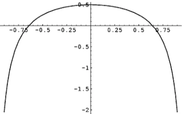
UsingMATHEMATICA, one has the following graphs for the function rp: Case p = 1 + 10−1_{; see Fig. 1;}

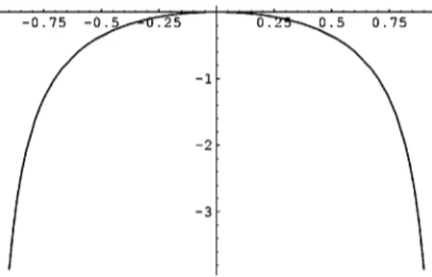
Case p = 1 + 10−6_{; see Fig. 2.}

Let us emphasize what we said in the Introduction: a recent result of Andai3 shows the nontriviality of the above behavior. Indeed, also in the 2⫻2 case there exist many monotone metrics with nonincreasing scalar curvature.

ACKNOWLEDGMENTS

It is a pleasure to thank J. Dittmann for discussions on the subject and especially for the proof of Theorem 7.1. We are indebted to P. Michor for some references and comments on scalar curvature.

1

Albert, P. M. and Uhlmann, A., “Stochasticity and partial order. Doubly stochastic maps and unitary mixing,” in Mathematics and its Applications共Reidel, Dordrecht, 1982兲, Vol. 9.

2

Amari, S. and Nagaoka, H., Methods of Information Geometry共American Mathematical Society, Providence, RI, 2000兲. 3

Andai, A., “Monotone Riemannian metrics on density matrices with nonmonotone scalar curvature,” J. Math. Phys. 44, 3675–3688共2003兲.

4

Andai, A., “On the monotonicity conjecture for the curvature of the Kubo–Mori metric,” math-ph/0310064v1. 5

Ando, T., “Majorization, doubly stochastic matrices, and comparison of eigenvalues,” Linear Algebr. Appl. 118, 163– 248共1989兲.

6

Ando, T., “Majorization and inequalities in matrix theory,” Linear Algebr. Appl. 199, 17–67共1994兲. 7

Bhatia, R., Matrix Analysis, Graduate Texts in Mathematics, 169共Springer, New York, 1997兲. 8

Brody, D. and Hughston, L., “Geometrization of statistical mechanics,” Proc. R. Soc. London, Ser. A 455, 1683–1715

共1999兲.

9

Brody, D. and Rivier, N., “Geometrical aspects of statistical mechanics,” Phys. Rev. E 51, 1006–1011共1995兲. 10_{Čencov, N. N., Statistical Decision Rules and Optimal Inference}

共American Mathematical Society, Providence, RI, 1982兲关translation from the Russian edited by Lev J. Leifman兴.

11

Dittmann, J., “The scalar curvature of the Bures metric on the space of density matrices,” J. Geom. Phys. 31, 16–24

共1999兲.

12

Dittmann, J., “On the curvature of monotone metrics and a conjecture concerning the Kubo–Mori metric,” Linear Algebr. Appl. 315, 83–112共2000兲.

13

Dittmann, J., personal communication, 2002. 14

Gibilisco, P. and Isola, T., “Connections on statistical manifolds of density operators by geometry of noncommutative Lp_{-spaces,” Infinite Dimen. Anal., Quantum Probab., Relat. Top. 2, 169–178}_共1999兲.

15

Gibilisco, P. and Isola, T., “Monotone metrics on statistical manifolds of density matrices by geometry of noncommu-tative L2_{-spaces,” in Disordered and Complex Systems, AIP Conference Proceedings 553, edited by P. Sollich et al.}_共AIP, Melville, NY, 2001兲, pp. 129–139.

16

Gibilisco, P. and Isola, T., “A characterisation of Wigner-Yanase skew information among statistically monotone met-rics,” Infinite Dimen. Anal., Quantum Probab., Relat. Top. 4, 553–557共2001兲.

(14)

17

Gibilisco, P. and Isola, T., “Wigner–Yanase information on quantum state space: The geometric approach,” J. Math. Phys.

44, 3752–3762共2003兲. 18

Gibilisco, P. and Isola, T., “On the characterization of paired monotone metrics,” Ann. Inst. Stat. Math. 56, 369–381

共2004兲.

19

Gibilisco, P. and Pistone, G., “Connections on nonparametric statistical manifolds by Orlicz space geometry,” Infinite Dimen. Anal., Quantum Probab., Relat. Top. 1, 325–347共1998兲.

20

Gibilisco, P. and Pistone, G., “Analytical and geometrical properties of statistical connections in information geometry,” in Mathematical Theory of Networks and Systems, edited by A. Beghi et al.共Il Poligrafo Padova, Italy, 1999兲, pp. 881–914

21

Grasselli, M. R., “Dual connections in nonparametric classical information geometry,” math-ph/0104031. 22

Hasegawa, H., “Dual geometry of the Wigner–Yanase–Dyson information content,” Infinite Dimen. Anal., Quantum Probab., Relat. Top. 6, 413–430共2003兲.

23

Hasegawa, H. and Petz, D., “Noncommutative extension of the information geometry II,” in Quantum Communications and Measurement共Plenum, New York, 1997兲, pp. 109–118.

24

Hiai, F., Petz, D., and Toth, G., “Curvature in the geometry of canonical correlation,” Stud. Sci. Math. Hung. 32, 235–249共1996兲.

25

Janke, W., Johnston, D. A., and Kenna, R., “Information geometry of the spherical model,” Phys. Rev. E 67, 046106

共2003兲.

26

Janyszek, H., “On the geometrical structure of the generalized quantum Gibbs states,” Rep. Math. Phys. 24, 11–19

共1986兲.

27

Janyszek, H. and Mrugala, R., “Riemannian geometry and the thermodyamics of model magnetic systems,” Phys. Rev. A 39, 6515–6523共1989兲.

28

Jenčová, A., “Geometry of quantum states: Dual connections and divergence functions,” Rep. Math. Phys. 47, 121–138 共2001兲.

29

Kriegl, A. and Michor, P. W., The Convenient Setting of Global Analysis, Mathematical Surveys and Monographs, Vol. 53共American Mathematical Society, Providence, RI, 1997兲.

30

Lieb, E. H., “Some convexity and subadditivity properties of entropy,” Bull. Am. Math. Soc. 81, 1–14共1975兲. 31

Marshall, A. W. and Olkin, I., Inequalities: Theory of Majorization and its Applications, Mathematics in Science and Engineering, 143共Academic, New York, 1979兲.

32

Michor, P., Petz, D., and Andai, A., “On the curvature of a certain Riemannian space of matrices,” Infinite Dimen. Anal., Quantum Probab., Relat. Top. 3, 199–212共2000兲.

33

Neuwirther, M., “Submanifold geometry and hessians on the pseudo-Riemannian manifold of metrics,” Acta Math. Univ. Comen. 52, 51–85共1993兲.

34

Petz, D., “Geometry of canonical correlation on the state space of a quantum system,” J. Math. Phys. 35, 780–795

共1994兲.

35

Petz, D., “Monotone metrics on matrix spaces,” Linear Algebr. Appl. 244, 81–96共1996兲. 36

Petz, D., “Covariance and Fisher information in quantum mechanics,“ J. Phys. A 35, 929–939共2002兲. 37

Petz, D. and Hasegawa, H., “On the Riemannian metric of␣-entropies of density matrices,” Lett. Math. Phys. 38, 221–225共1996兲.

38

Petz, D. and Sudár, C., “Geometry of quantum states,” J. Math. Phys. 37, 2662–2673共1996兲. 39

Ruppeiner, G., “Riemannian geometry approach to critical points: General theory,” Phys. Rev. E 57, 5135–5145共1998兲. 40

Ruskai, M. B., “Lieb’s simple proof of concavity of 共A,B兲哫Tr Ap_K†_B1−p_{K and remarks on related inequalities,”} quant-ph/0404126v1.

41