ALMA MATER STUDIORUM
UNIVERSITÀ DEGLI STUDI DI BOLOGNA
_____________________________________________________
Dipartimento di Fisica e Astronomia
DOTTORATO DI RICERCA IN
ASTROFISICA
Ciclo XXX
Tesi di Dottorato
STAR FORMATION HISTORIES IN THE NEARBY UNIVERSE:
THE HST LEGACY
Presentata da: Elena Sacchi
Coordinatore Dottorato:
Francesco Rosario Ferraro
Supervisore:
Monica Tosi
Co-supervisore:
Michele Cignoni
Esame finale anno 2018
_____________________________________________________
Settore Concorsuale: 02/C1 – Astronomia, Astrofisica, Fisica della Terra e dei Pianeti
iii
“Stars are beautiful, but they may not take an active part in anything, they must just look on for ever. It is a punishment put on them for something they did so long ago that no star now knows what it was. So the older ones have become glassy-eyed and seldom speak (winking is the star language), but the little ones still wonder.”
A
BSTRACT
This thesis has been devoted to a research project selected and funded by INAF (the Italian National Institute for Astrophysics) within the framework of the formal agreement between INAF and the Bologna University for the PhD program in As-trophysics.
The aim of the project is to study star-forming galaxies in the local Universe, and in particular the distribution of their stellar populations and their star formation histories, to understand how the clustering of star formation evolves both in space and time.
The data I analyzed have been acquired with the Hubble Space Telescope (HST), whose spatial resolution and sensitivity allow to measure individual stars with the highest possible accuracy even in crowded and relatively distant galaxies. Thanks to its exquisite performances, HST is still the most powerful facility for this kind of studies.
The method I used to derive the star formation histories of the examined galaxies is based on the color-magnitude diagram (CMD), one of the best information desks on the evolution of a galaxy or stellar system. More specifically, I applied to the ob-servational color-magnitude diagrams the synthetic CMD technique, a reliable tool to explore the detailed star formation history of nearby galaxies and refine stellar evolution models by comparing them with the data. This method was implemented in the code SFERA, which I have contributed to improve and that will be extensively described in this thesis.
Within this framework, I discuss the results obtained for three galaxies of different morphological type which have been targeted by the HST Treasury program LEGUS (Legacy ExtraGalactic Ultraviolet Survey), a large international collaboration whose aim is to investigate and connect the different scales of star formation, from young stellar clusters to local Universe galaxies. The galaxies I analyze are DDO 68, a dwarf irregular, NGC 4449, a Magellanic irregular, and NGC 7793, a flocculent spi-ral, which were studied both in the UV and optical bands, in order to recover their star formation histories from very recent to older epochs and to understand whether and how the star formation process may depend on the morphological, dynamical and environmental properties of the galaxies.
vii
C
ONTENTS
Abstract v
List of Abbreviations ix
1 Introduction 1
1.1 The context: galaxies in the local Universe . . . 1
1.2 Star Formation Histories of nearby galaxies . . . 4
1.3 A new survey: LEGUS . . . 11
2 From theory to practice 13 2.1 The Color-Magnitude Diagram and its power . . . 13
2.1.1 Age indicators on a CMD . . . 16
2.1.2 Optical versus UV . . . 18
2.2 The synthetic CMD method: strengths and uncertainties . . . 21
2.2.1 How to build a synthetic CMD: the SFERA approach . . . 21
2.2.2 Comparing models and data . . . 22
2.2.3 All kinds of uncertainties . . . 23
2.3 Matching the two worlds: SFERA . . . 30
2.3.1 Time resolution tests . . . 31
3 The dwarf: DDO 68 35 3.1 Observations and Data Reduction . . . 38
3.2 Incompleteness and Errors . . . 40
3.3 The Color-Magnitude Diagram . . . 42
3.4 Distance Determination . . . 45
3.5 Stellar populations in DDO 68 . . . 47
3.5.1 Spatial distribution . . . 47
3.5.2 HIIregions . . . 49
3.6 Star Formation History . . . 51
3.6.1 Basis Functions . . . 51 3.6.2 REGION1 . . . 53 3.6.3 REGION2 . . . 54 3.6.4 REGION3 . . . 57 3.6.5 REGION4 . . . 57 3.6.6 DDO 68 B . . . 59
3.7 A Flea with Smaller Fleas that on Him Prey . . . 61
3.7.1 Physical properties of the substructures . . . 63
3.7.2 Dynamics of DDO 68 . . . 64
4 The starburst: NGC 4449 69
4.1 Observations and Data . . . 70
4.2 Artificial Star Tests . . . 72
4.3 Distribution of the stellar populations . . . 74
4.4 The UV perspective . . . 77
4.5 Star Formation History . . . 80
4.5.1 Whole galaxy . . . 80 4.5.2 Central fields . . . 86 4.5.3 External fields . . . 91 4.6 Results . . . 98 4.7 Discussion . . . 100 5 The spiral: NGC 7793 103 5.1 Observations and Data . . . 104
5.2 Distribution of the stellar populations . . . 107
5.3 Distribution of dust . . . 110
5.4 Star Formation History . . . 112
5.4.1 Inner region . . . 112
5.4.2 Middle region . . . 113
5.4.3 Outer region . . . 113
5.5 Discussion . . . 117
6 A picture of Star Formation in nearby Galaxies 121 6.1 Three different galaxies: a comparative study . . . 123
6.2 The Schmidt-Kennicutt law . . . 127
6.3 The Role of Interaction . . . 132
7 Concluding remarks 135
Acknowledgements 137
L
IST OF
A
BBREVIATIONS
ACS Advanced Camera for Surveys AGB Asymptotic Giant Branch
ALMA Atacama Large Millimeter Array ANGST ACS Nearby Galaxy Survey Treasury
AST Artificial Star Test BCD Blue Compact Dwarf
BF Basis Function BL Blue Loop BSG Blue SuperGiant
CMD Color-Magnitude Diagram CMF Cumulative Mass Fraction
CTE Charge Transfer Efficiency dE dwarf Elliptical
dIrr dwarf Irregular DM Distance Modulus dSph dwarf Spheroidal dTrans dwarf Transition type
FoV Field of View
GMC Giant Molecular Cloud H-R Hertzsprung-Russell
HB Horizontal Branch HST Hubble Space Telescope
IMF Initial Mass Function ISM InterStellar Medium LBC Large Binocular Camera LBT Large Binocular Telescope
LCID Local Cosmology from Isolated Dwarfs LEGUS Legacy ExtraGalactic UV Survey
LF Luminosity Function LG Local Group
LMC Large Magellanic Cloud MS Main Sequence
MSTO Main Sequence Turn Off MW Milky Way
NNLS Non-Negative Least-Square PSF Point Spread Function
RC Red Clump RGB Red Giant Branch
x
SC Stellar Cluster
SED Spectral Energy Distribution SF Star Formation
SFE Star Formation Efficiency
SFERA Star Formation Evolution Recovery Algorithm SFH Star Formation History
SFR Star Formation Rate SGB SubGiant Branch
SK Schmidt-Kennicutt SMC Small Magellanic Cloud
TP-AGB Thermally Pulsing Asymptotic Giant Branch TRGB Tip of the Red Giant Branch
uFd ultraFaint dwarf UVIS UV/VISible channel
VLA Very Large Array WFC Wide-Field Channel WFC3 Wide-Field Camera 3
WFPC2 Wide-Field Planetary Camera 2 WR Wolf-Rayet
xi
Dedicated to my parents and my sister, there for me, always and ever. Ai miei genitori e mia sorella, che ci sono e ci saranno per me, sempre.
1. I
NTRODUCTION
1.1 The context: galaxies in the local Universe
The local Universe is characterized by a great variety of galaxies and galactic en-vironments. Within the Local Group (LG), we find spirals, Andromeda and the Milky Way (MW) being the biggest ones, their numerous satellites, mainly dwarf spheroidal (dSph), dwarf irregular (dIrr) and ultrafaint dwarf (uFd) galaxies, and several other dwarfs, apparently not connected to larger systems. Going beyond, within a few tens of Mpc from the Milky Way, we find entirely new classes of very interesting galaxies, such as radio galaxies and Seyferts, those with the lowest star formation activity (early-type ellipticals), and those with the highest one (starburst late-type galaxies), including dwarfs as the blue compact dwarfs (BCDs), very active star-forming galaxies characterized by high gas contents and very low metallicities. Among all these morphological types, dwarf galaxies are the most common but probably least understood objects when we consider their formation and evolution. As for elliptical and spiral galaxies, we can divide dwarfs on the basis of their activity and gas content in early-type, i.e. dSphs and dwarf ellipticals (dEs), and late-type, including dIrrs and BCDs; the uFd class is still poorly defined, because of the low number of these galaxies found so far and of their properties, compatible with those of both low luminosity dwarf galaxies and faint diffuse globular clusters. Even in the comparison among dwarfs of the same class, we find a wide range of chemi-cal, dynamical and star formation (SF) properties, and the evolutionary processes taking place in these systems are still highly debated, as much as the definition of dwarf galaxy itself. Tolstoy, Hill, and Tosi (2009) review the main characteris-tics of dwarf galaxies in the Local Group, investigating possible connections and correlations among their different properties. In particular, despite the differences, they suggest an evolutionary sequence connecting early-type and late-type dwarfs, though strongly affected by environmental effects. Indeed, if we look at how some structural parameters are related in different kinds of galaxies, such as half-light ra-dius (re), surface brightness (µe) and absolute magnitude (MV), we find a rather con-tinuous distribution from early- to late-type galaxies (Kormendy and Bender,2012). Figure 1.1 shows this parameter correlations for spheroidal and late-type galaxies, confirming their close connection. However, a deep understanding of this relation is still lacking, as well as a clear evolutionary process linking the different types of galaxies.
A crucial information to understand galaxy formation and evolution is the star for-mation history (SFH), which is the result of gas consumption, chemical enrichment and interaction processes experienced by a galaxy. For nearby galaxies, we have the great advantage of resolving their stellar populations, so that we are able to
2 Chapter 1. Introduction
FIGURE1.1: Relations among structural properties of different kinds of galaxies Top panel. Surface brightness µe at the effective radius versus absolute magni-tude MV. Bottom panel. Effective radius reversus absolute magnitude. Different galaxy types are marked with different colors: ellipticals (pink), classical bulges (light brown), pseudo-bulges (light blue), spiral disks and irregulars (blue), and spheroidals (green). See Figure 20 of Kormendy and Bender (2012) for more
1.1. The context: galaxies in the local Universe 3 perform spatially resolved studies revealing the variations of their SFH as a func-tion of posifunc-tion, populafunc-tion and metallicity gradients, formafunc-tion and merger history. Most galaxies show these variations, with old populations being found everywhere whereas the young ones are usually more centrally concentrated or confined to disks and spiral arms.
From a cosmological point of view, the hierarchical formation scenario suggests that big galaxies form through continuous merging and accretion of smaller building blocks. As a consequence, present-day dwarfs may have been sites of the earli-est star formation activity in the Universe. On the other hand, given their high gas content and very blue integrated colors, indicative of the prevalence of young stellar populations, the most metal-poor (12 + log(O/H) . 7.6, corresponding to Z . 1/15 Z 1) dwarf irregular and blue compact dwarf galaxies have been often suggested to be “primeval” galaxies, experiencing their first burst of star forma-tion, with ages. 100 500 Myr (Izotov and Thuan, 1999; Pustilnik, Kniazev, and Pramskij,2005; Pustilnik, Tepliakova, and Kniazev,2008). However, all dIrr/BCD galaxies resolved and studied so far with the Hubble Space Telescope (HST) have been found to harbor stars as old as the look-back time sampled by the depth of the photometry, i.e. ⇠ 1 Gyr and older (Tolstoy et al.,1998; Schulte-Ladbeck et al.,
2002; Izotov and Thuan,2002; Tosi,2009; Tolstoy, Hill, and Tosi,2009). The signifi-cance of such studies is clearly illustrated in the long-standing controversial case of I Zw 18, one of the most metal-poor star forming dwarfs and the prototype of the BCD class with 12 + log(O/H) = 7.2 (Skillman and Kennicutt,1993). Imaging with the Advanced Camera for Surveys (ACS) on board of HST performed by Aloisi et al. (2007) provided a deep and uncontaminated color-magnitude diagram (CMD) that indisputably demonstrated the presence of a previously uncertain red giant branch (RGB), thus ruling out its former classification as a truly primordial galaxy (Izotov and Thuan,2004).
Over the past years, several new dIrr/BCDs with extremely low metallicities and physical properties similar to those of I Zw 18 have been discovered and controver-sially regarded as “genuine” young galaxies in the nearby Universe, due to a lack of detailed information on their resolved stellar population ages. One of the most recent cases is Leo P, discovered by Giovanelli et al. (2013) within the ALFALFA survey, with a metallicity from HII region spectra of 12 + log(O/H) = 7.17 ± 0.04
(Skillman et al.,2013). McQuinn et al. (2015) observed it with HST and indisputably found RR Lyrae stars, i.e. stars at least 10 Gyr old, from which they also inferred a robust distance estimate of 1.62 ± 0.15 Mpc.
One effective way to check whether or not big galaxies are made only by succes-sive accretions of smaller satellites is to compare the property of massucces-sive and dwarf systems. If chemical abundances, kinematics, and star formation histories of the re-solved stars of massive galaxies are all consistent with those of dwarf galaxies, then the former can be the result of successive merging of the latter; otherwise, either satellite accretion is not the only channel to build up spiral and elliptical galaxies or the actual building blocks are not alike today’s dwarfs.
4 Chapter 1. Introduction
1.2 Star Formation Histories of nearby galaxies
The study of nearby galaxies has been revolutionized by the Hubble Space Tele-scope. Its high spatial resolution allowed for the first time to resolve and measure individual stars even in the crowded fields of external galaxies and to draw their CMDs, permitting studies of stellar populations, star formation histories, and stellar clusters for galaxies out to several Mpc. The CMD of a stellar system is in fact one of the best information desks on the system evolution, because it preserves the im-printing of all the relevant evolution parameters, such as age, mass, chemical com-position, initial mass function (IMF).
Deep CMDs display all the stars still alive born over the whole lifetime of a galaxy, and are indeed fossil records of the SFH. A first qualitative idea of the stellar pop-ulations in a galaxy can be obtained simply by looking at a good CMD. Different evolutionary phases trace different epochs: RR Lyrae stars are indicative of a very old population; red giant branch stars are associated with intermediate-age to old star formation activity; asymptotic giant branch (AGB) stars can span from old to intermediate and young ages; the blue, brightest stars, as well as HIIregions, are
evidence of very recent star formation activity.
Up to the early ’90s, stellar ages were derived through isochrone fitting, a simple and effective method to determine the age and metallicity of single stellar populations such as the ones in star clusters, but inadequate to interpret the multiple popula-tions of galaxies, where many different generapopula-tions of stars can contribute to the morphology of the observed CMD.
A more sophisticated and quantitative technique was then developed by Tosi et al. (1991), the synthetic CMD method, that consists in the extrapolation of the standard isochrone fitting method by creating theoretical CMDs via Monte Carlo extractions from an isochrone set, and comparing them to the observed CMD. It includes the estimate of photometric errors, completeness and crowding, and it is still the most powerful technique available for this kind of analysis and, in general, for SFH stud-ies of resolved stellar populations. A detailed description of this method will be presented in the next Chapter.
One of the first surveys creating a uniform archive of resolved galaxies is the ACS
Nearby Galaxy Survey Treasury (ANGST) program (Dalcanton et al.,2009). They
built a sample of 69 galaxies within a radius of 3.5 Mpc and included the M81 group (at 3.6 Mpc) and the BGC 253 clump in the Sculptor group (at 3.9 Mpc) to cover a wider morphology and environment range. 60 of these are dwarf galaxies, including 12 dwarf spheroidal/dwarf elliptical galaxies, 5 dwarf spirals, 28 dwarf irregulars, 12 dwarf transition type (dTrans) galaxies and 3 tidal dwarfs. Weisz et al. (2011) an-alyzed this dwarf sub-sample and uniformly derived the SFHs using the synthetic CMD method. The ANGST dwarf galaxies exhibit a wide variety of complex SFHs, but the mean SFHs of the different morphological types are generally indistinguish-able earlier than the most recent ⇠ 1 Gyr. On average, they find that the typical dwarf galaxy formed the bulk of its stars prior to z ⇠ 1, although the uncertainties are relatively large, particularly for dIrrs, which have very different SFHs. Figure 1.2 shows their resulting cumulative SFHs. Despite the variety of the individual curves,
1.2. Star Formation Histories of nearby galaxies 5 the mean trends are remarkably similar, and the clearest differences between the morphological types arise in the most recent 1 Gyr, where the typical dSph, dTrans, dwarf spiral and dIrr galaxies formed an increasing amount of their total stellar mass (⇠ 2%, 4%, 5% and 8% respectively).
FIGURE1.2: Cumulative SFHs of the ANGST sample of dwarf galaxies, divided
per morphological type. The horizontal dot-dashed line represents 50% of the total stellar mass. Excluding the tidal dwarfs, most dwarf galaxies appear to have formed the bulk of their stellar mass prior to z ⇠ 1. See Figure 5 of Weisz et al.
(2011) for more details.
A smaller but more precise program was presented by Gallart (2008) and Hidalgo et al. (2013), the Local Cosmology from Isolated Dwarfs (LCID) project, also based on HST/ACS observations. They wanted to study the detailed SFHs of six isolated dwarf galaxies of the Local Group, two dIrrs, IC1613 and Leo A, two dTrans, LGS3 and Phoenix, and two dSphs, Cetus and Tucana, in order to investigate the effects of phenomena that may affect the early evolution of dwarf galaxies in the absence of
6 Chapter 1. Introduction strong environmental effects; subsequently, another dIrr galaxy, DDO210, has been studied (Cole et al.,2014). As shown in Figure 1.3, they find that Tucana and Cetus share the common characteristic of having formed over 90% of their stars before
10Gyr ago, and they host no stars younger than 8 9 Gyr. The SFHs of the two
dTrans galaxies are remarkably similar to those of the dSphs: they formed over 80% of their stars before 9 Gyr ago in spite of having maintained residual star formation during the rest of their evolution. The lower panel of the figure displays the SFHs of the two dIrrs in their sample, Leo A and IC1613. In contrast to the former SFHs, those of the dIrrs do not show a dominant early burst of star formation; instead, over 60%of their stars formed at intermediate and young ages.
FIGURE1.3: SFHs of the six LCID galaxies. Top panel. SFHs of the dSphs (red) and dTrans (magenta). Bottom panel. SFHs of the dIrrs. See Figure 1 of Gallart et al.
(2015) for more details.
Gallart et al. (2015) make a very interesting analysis comparing these six isolated dwarfs with dwarfs that are, at present, found close to the large spirals, with SFHs from the literature. Most MW satellites (UMi, Draco, Sextans, Scl, CnVI, plus the very faint dwarfs, Brown et al., 2014) formed most of their stars before ⇠ 10 Gyr ago. The more distant dSph satellites, Fornax, Leo I, and Carina, show substantial intermediate-age populations: their SFHs peaked at ages younger than 10 Gyr, and
1.2. Star Formation Histories of nearby galaxies 7 most of their star formation occurred at intermediate ages. In fact, the SFHs of these dSphs are similar to those of dIrr galaxies for most of their lifetimes: they have low initial star formation rates (SFRs) and high SFRs at intermediate ages. The main difference occurs in the last ⇠ 2 Gyr or less, when their star formation stopped. They are classified as dSphs for their current properties, but their history is similar to that of dIrr galaxies. Based on their full evolutionary histories, they propose a new classification for dwarf galaxies, that can be grouped in two classes (see Figure 1.4):
• fast dwarfs that started their evolution with a dominant star formation event, but their period of star formation activity was short (few Gyr);
• slow dwarfs that formed a small fraction of their stellar mass at an early epoch, and continued forming stars until the present (or almost).
FIGURE1.4: SFHs of Local Group fast (top panel) and slow (bottom panel) dwarfs. Note that in the bottom panel both slow dwarfs currently classified as dSphs (in green shades) and dIrrs (in blue shades) are represented. See Figure 2 of Gallart
8 Chapter 1. Introduction These two evolutionary paths do not correspond directly to the current, commonly adopted dwarf galaxy classification (in dIrrs, dTrans and dSphs). Most notably, some dSphs have important intermediate-age and young populations, and thus SFHs that resemble those of dIrrs: in this sample, all dIrrs are slow dwarfs, while some dSphs are fast and others are slow. In addition to SFHs, slow and fast dwarfs also differ in their inferred early location relative to the local large galaxies: as opposed to fast dwarfs, slow dwarfs’ positions and radial velocities are compatible with a late first infall into the Local Group, which would imply that they were assembled in lower-density environments than fast dwarfs. They thus suggest that the nature of fast or slow dwarfs is determined by the formation conditions of the galaxy, when the environment influenced the mass-assembly process of the dwarf (which is expected to depend on the formation location) rather than removing the gas later. In this scenario, the progenitor halos of fast dwarfs assembled early and quickly in high-density environments, where interactions triggering star formation were common, likely leading to high SFRs even before reionization. Strong gas loss would follow as a consequence of the effects of reionization and feedback acting together. Slow dwarfs resulted from delayed, slower mass assembly occurring in lower-density en-vironments, which in turn led to a delayed onset of star formation, occurring when the halo had grown massive enough to allow the gas to cool and form stars. This implies milder feedback and gas loss, and the possibility of keeping forming stars on a long timescale. A strong interaction with a large host could play a role in the fi-nal removal of gas from the dwarf galaxies that infall late. The morphology-density relation observed (with exceptions) in LG dwarf galaxies today would thus be a con-sequence of their formation in more or less dense environments around the LG. A more extended study of LG dwarf galaxies was made by Weisz et al. (2014), who analyzed a sample of 40 galaxies located within ⇠ 1 Mpc and observed with the HST/Wide-Field Planetary Camera 2 (WFPC2). This sample consists of 23 dwarf spheroidals, 4 dwarf ellipticals, 8 dwarf irregulars, and 5 transition dwarfs. Figure 1.5 shows their results. They find several interesting trends for each morphological type, here summarized.
• dSphs are predominantly old systems and have formed the vast majority of their stars prior to z ⇠ 2 (10 Gyr ago). However, while this behavior holds on average, the individual galaxies show a significant scatter, ranging from purely old to those with nearly constant lifetime SFHs.
• There are few predominantly old dIrrs. On average, dIrrs formed ⇠ 30% of their stellar mass prior to z ⇠ 2, and show an increasing SFR toward the present, beginning around z ⇠ 1 (7.6 Gyr ago). This behavior is generally reflected in the SFHs of individual dIrrs, which show only modest scatter rela-tive to the average.
• On average, dTrans appear to have formed 45% of their total stellar mass prior to z ⇠ 2, and have experienced nearly constant SFRs since that time. The SFHs of the individual galaxies show modest scatter over most of their lifetimes. • dTrans with predominantly old SFHs tend to have lower present day gas
frac-tions, while those with higher gas fraction have had more constant SFHs over most of their lifetimes.
1.2. Star Formation Histories of nearby galaxies 9 • dEs typically have an initial burst of star formation prior to ⇠ 12 Gyr ago, fol-lowed by a nearly constant SFR. They show little scatter relative to the average value, and all exhibit declining SFHs starting at z ⇠ 0.1 (2 Gyr ago).
FIGURE 1.5: Unweighted average cumulative SFHs of 40 Local Group dwarf
galaxies, grouped by morphological type (dSph red, dIrr blue, dTrans orange, dE green). Top panels. The solid line represents the median value of the SFH with the statistical uncertainties, while the gray lines are the individual SFHs. Middle panels. Average SFHs with uncertainties given by the root square sum of the differ-ential ensemble systematics and the standard error in the median. Bottom panels. Average SFHs with 3 simple SFH models over plotted. See Figure 9 of Weisz et al.
(2014) for more details.
As shown in the middle panels of the figure, on average, all morphological types formed ⇠ 30% of their stars prior to 12 Gyr, and are only statistically different after this epoch. In the bottom panels, the average SFHs is compared with simple SFH models (single old population, exponentially declining “⌧-models”, and constant). The best matches are with the dSphs, whose average SFH is well-approximated by a ⌧-model with ⌧ = 5 Gyr. Instead, dIrrs, dTrans, and dEs all show a modest initial burst in their SFHs (> 10 12 Gyr ago) followed by nearly constant or slightly rising
SFHs. The combination of an exponential SFH (⌧ = 3 5Gyr) prior to 10 12Gyr
ago, followed by a constant SFH thereafter provides a reasonable approximation for the average SFHs of these three groups.
10 Chapter 1. Introduction Given their very privileged position very close to the MW, the Magellanic Clouds are another fundamental target for stellar population studies outside our galaxy. They are two interacting satellites of the Milky Way, the Large Magellanic Cloud (LMC) and the Small Magellanic Cloud (SMC), an irregular galaxy at the boundary of the dwarf class. In particular, the SMC can be considered the closest late-type dwarf, given its high gas content, low metallicity (Z ⇠ 0.004), and low mass (1 5 ⇥ 109 M ) near the upper limit of the range of masses typical of late-type dwarfs (Tol-stoy, Hill, and Tosi, 2009). The first determination of the full, global SFH of the SMC (through the synthetic CMD method), was made by Harris and Zaritsky (2004), thanks to the Magellanic Clouds Photometric Survey (Zaritsky, Harris, and Thomp-son,1997), a spatially comprehensive catalog of their stellar populations. However, their ground-based photometry did not reach the oldest main sequence turn off, and this hampered the derivation of the SFH at relatively early epochs. Subsequent deeper studies, as Noël et al. (2009), Cignoni et al. (2013), and Weisz et al. (2013), found that for ages > 12 Gyr, the SFH of the SMC is consistent with a constant life-time SFH, suggesting either suppressed or under-fueled star formation, relative to other Milky Way satellites at comparable distances; two distinct SF peaks are present at ⇠ 4.5 and 9 Gyr, which may be due to periodic encounters with the LMC, while the LMC had roughly constant star formation at the same epochs; at ⇠ 3.5 Gyr ago both galaxies show a sharp increase in SFR, and their SFHs track each other sub-sequently, consistent with suggestions of a close encounter with the Milky Way at recent times; starting around ⇠ 3.5 Gyr ago, the SF in the outer regions of the SMC abruptly ceases, while the SFR in the galaxy’s center sharply increases, suggesting gas from the outer regions has been centrally funneled.
Another study of nearby dwarf galaxies is the one performed by McQuinn et al. (2010), not based on a specifically designed survey but on archival HST observations. They select 18 starburst dwarfs covering a range of brightness, morphologies, and spatial extent, in order to explore the starburst phenomenon in relation to different dwarf galaxy properties. Their SFH derivation shows large variations from galaxy to galaxy, and, while their sample includes a class of objects undergoing significant recent SF, they do not find a common SFR profile that characterizes the starburst phe-nomenon. In most of their galaxies, elevated levels of SF are sustained over a large interval of time ( t > few 100 Myr), and there are variations and inhomogeneities in the SFR profiles on small temporal scales ( t ⇠ 10 20 Myr).
The great variety of dwarf galaxies within and outside the Local Group, once again underlines the complexity of this class of objects, and the strong need for detailed studies of their kinematics, metallicities, stellar contents and evolution.
1.3. A new survey: LEGUS 11
1.3 A new survey: LEGUS
The Legacy ExtraGalactic UV Survey (LEGUS) is a Hubble Space Telescope Cycle 21 Treasury program (GO 13364, PI D. Calzetti), whose aim is to provide a homoge-neous imaging data set in five bands (from the near ultraviolet to the near infrared) of a sample of 50 local (closer than 12 Mpc) star-forming galaxies. These targets have been selected to sample a full range of global galactic properties such as morphology, star formation rate, mass, metallicity, internal structure, and interaction state, repre-sentative of the variety observed within the Local Volume (Calzetti et al.,2015). The main scientific goal of the survey is to link the different scales of star formation, from stellar associations to galaxies, and in particular to investigate how the clustering of star formation evolves both in space and in time, discriminate among different mod-els of star cluster evolution, explore the effects of SFH on the UV star formation rate calibrations, quantify the impact of the environment on star formation and cluster evolution across the full range of galactic and interstellar medium properties. The LEGUS images were obtained with the Wide-Field Camera 3 (WFC3), in the filters F275W ( 2704 Å), F336W ( 3355 Å), F438W ( 4325 Å), F555W ( 5308 Å), and F814W ( 8024 Å), plus parallel optical imaging with the ACS, in the filters F435W ( 4328 Å), F606W ( 5921 Å), and F814W ( 8057 Å). Figure 1.6 shows the full LEGUS sample.
Thanks to the multi-band imaging, the LEGUS photometry covers both blue and red, young and old stellar populations, in the field as well as in clusters. Hence, compar-isons between recent (. 50 Myr) and ancient star formation histories from resolved stellar populations are possible, as well as the investigation of the spatial and tempo-ral evolution of star formation within the galaxies. This can eventually improve the theoretical scenarios on galaxy evolution and help to really understand the physical processes connecting gas and star formation, and possibly their evolution in dif-ferent environments and at high redshift. One of the goals of LEGUS is to enable accurate ( (age)/age ⇡ 10% 20%) determinations of SFHs in its sample galaxies. The LEGUS UV observations resolve the majority of stars above ⇡ 7 10 M at all the considered distances, in the disks and in sparse groups and OB associations; the outer regions of star clusters can be partially resolved in the closest (< 5 6Mpc) galaxies. Using the UV and U bands, we can build color-magnitude diagrams where the main sequence (MS) stars and the blue loop (BL) core helium-burning stars are separated in two cleaner sequences with respect to the optical CMDs, where these stars partially overlap (Tolstoy et al.,1998). With this separation, the correspondence between luminosity and age that is found for BL stars can be a strong constraint to directly convert the luminosity function into the SFH (see Section 2.1). Comparison among different bands can also help to model the extinction and differential redden-ing that can heavily affect gas- and dust-rich galaxies, and even put constraints on the shape of the stellar IMF.
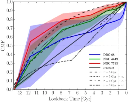
As a member of the LEGUS collaboration, I am in charge of deriving accurate and reliable SFHs of a subsample of the 50 LEGUS galaxies. The idea was to analyze dif-ferent galaxy types with a smooth transition from the smallest dwarfs to the biggest spirals. In this thesis, we use LEGUS’ data to derive the SFH of three galaxies of different type: a dwarf irregular, DDO 68, a Magellanic irregular, NGC 4449, and
12 Chapter 1. Introduction
FIGURE 1.6: The full 50 galaxies LEGUS sample shown with GALEX two-color
(far-UV and near-UV) images. The two bars under the galaxy name indicate the angular (1’, red bar) and physical (1 kpc, white bar) scale. See Calzetti et al. (2015)
for more details.
a flocculent spiral, NGC 7793. Given the longer timescale covered and the need to build a homogeneous archive to refer to in all future applications, the analyses of the optical stellar populations and SFHs of these galaxies are the first we approached. The corresponding study in the UV and U bands has been carried out in parallel by other members of the team, and will be briefly presented in what follows, as prelim-inary results.
2. F
ROM THEORY TO PRACTICE
2.1 The Color-Magnitude Diagram and its power
One of the most useful and fundamental plots in stellar astronomy is the Hertzsprung-Russell (H-R) diagram, which illustrates the relation existing between effective temperature and luminosity of a star. Thanks to the Stefan-Boltzmann
equation L = 4⇡R2 T4
e (where L, R and Te are the star luminosity, radius and effective temperature, respectively, and = 5.67 ⇥ 10 5 erg cm 2K 4s 1 is the Stefan-Boltzmann constant), the location of any star of given radius and temperature in the H-R diagram is uniquely defined. This makes the H-R diagram the plot of reference to study stellar evolution.
In practice, the luminosity of a star is commonly measured on a logarithmic scale, going back to the first classification by Hipparchus that divided the observable stars in different classes according to their apparent magnitude m. Luminosity and ap-parent magnitude of a star are related by:
m = 2.5 log10 L
4⇡d2 + c (2.1)
where d is the star distance and c is a constant. Since the absolute magnitude is de-fined as the apparent magnitude of that star if located at 10 pc from us, the difference between the apparent and absolute magnitude M (the distance modulus, DM) is:
m M = 5 log10(d) 5 . (2.2)
Different stellar temperatures generate different sets of absorption lines, that trans-late into different spectral types such as O, B, A, F, G, K, M; another estimate of the temperature of a star comes from the so-called color index, which is the difference of the magnitude of the star in two different photometric filters (see Figure 2.1). The theoretical H-R diagram (log L/L vs log Te, where L = 3.83 ⇥ 1033 erg s 1 is the solar luminosity) and its observational counterpart, the color-magnitude di-agram (magnitude vs color index), display how luminosity and temperature (or magnitude and color) of a star of a given mass change as a function of time and therefore evolutionary phase (stellar evolution track) or alternatively how luminos-ity and temperature (or magnitude and color) of a star of a given age change as a function of its mass and therefore evolutionary phase (isochrone).
This tool gave a huge boost to understand how stars and groups of stars evolve, first of all showing that regardless of their mass, stars spend the majority of their lives in the main sequence phase, burning hydrogen in their core. At fixed age, MS
14 Chapter 2. From theory to practice
FIGURE2.1: Luminosity L (absolute magnitude MV) against effective temperature Te(color B V) of stars ranging from the high-temperature blue-white stars on the left side of the diagram to the low-temperature red stars on the right side. The x-axis is also labeled with the main spectral types. The plot includes the 22 000 stars from the Hipparcos Catalogue together with 1000 low-luminosity stars (red and white dwarfs) from the Gliese Catalogue of Nearby Stars. The core hydrogen burning stars are found in a band running from top-left to bottom-right (the main sequence). Giant stars form a clump on the upper-right side of the diagram. Above them lie the bright giants and supergiants. At the lower-left is the band of white
2.1. The Color-Magnitude Diagram and its power 15 stars follow a well-defined mass-luminosity relation, with L / M3 4. Moreover, the evolutionary timescale on the MS also depends on the mass, so that more massive stars live for shorter times while low-mass stars can sample the whole lifetime of a galaxy, with a relation that is roughly tM S / M 2.5. Thus, combining this two relations gives us a very important time-luminosity relation, i.e. the luminosity of a MS star on the CMD can be directly translated into an age. The intrinsic spread of the MS is given by both binaries and different metallicities in the stellar populations, so the blue edge of the zero age MS (ZAMS) corresponds to the minimum metallicity present in the galaxy, while the red edge is defined by the combination of higher metallicity MS stars with binary MS stars and stars evolving off the MS.
When all the hydrogen in the core has been converted into helium, the off-MS evolu-tion begins. Depending on the mass of the star, this phase can be quite different. In low-mass (M . 2 M ) stars the temperature in the core is not high enough to start the fusion of helium, so the core collapses reaching the status of electron degen-eracy, while the hydrogen fusion starts in a shell, making the star more luminous and accumulating more helium onto the degenerate core. This phase is called red giant branch and its shape and age are very sensitive to metallicity differences (age-metallicity degeneracy). When the helium core reaches M ⇠ 0.5 M the helium ignition starts violently, removing the degeneracy and producing the so-called he-lium flash, that suddenly ends the RGB phase and starts the horizontal branch (HB) phase (metal-poor stars) or red clump (RC) phase (metal-rich stars), where helium burning proceeds in the core. This process happens at fixed core mass, indepen-dently of the initial mass of the star, so the maximum luminosity reached during the RGB is almost constant, and it is called RGB tip (TRGB). This can be a very reliable distance estimator even in distant galaxies.
In intermediate-mass (2 M . M . 6 8 M 1) stars, the helium ignition in the
core happens in a non-violent way, and the stars describe large loops in color, the so-called blue loops. The BL luminosity is directly correlated to the total mass, since the mass of the core depends on the extension of the convective core in the previous MS phase, which in turn is a function of the total mass. This makes the blue loops very good age indicators. After the core helium burning phase, low and intermediate mass stars experience the asymptotic giant branch phase. The core is made of carbon and oxygen, as results of the helium burning, while two different shells burn helium (a more internal one) and hydrogen (a more external one). The star expands and develops an extended convective envelope, running almost parallel to the RGB. The shells alternatively stop and re-ignite the nuclear reactions, as the star expands and contracts, producing the so-called thermal pulses during thermally pulsing AGB (TP-AGB) phase. Both during the RGB and TP-AGB phases the stars experience a huge mass loss, that is still very hard to model and quantify.
High-mass stars (M& 8 15 M ) form in a small fraction in a galaxy because of the negative slope of the initial mass function (i.e. the distribution of initial masses for
1The boundary between intermediate- and high-mass stars depends on the evolutionary models.
Many groups define high-mass stars all those with a mass above 8 M , while the Padova group uses
6M as the highest mass intermediate-mass star, due to how they model the effect of overshooting,
16 Chapter 2. From theory to practice a population of stars), and their lifetimes are very short (< 20 Myr). Thus, they are indicative of recent or ongoing SF.
2.1.1 Age indicators on a CMD
To recover the SFH from the observational CMDs of the considered region through the comparison with synthetic models, the following ingredients are required:
• a set of stellar evolutionary tracks, providing the temperature and luminosity of stars in a (as fine as possible) grid of masses and metallicities according to their evolutionary time scales;
• stellar atmosphere models, to transform the bolometric magnitudes and tem-peratures into the observational plane;
• an initial mass function, regulating the number of stars born as a function of their mass;
• a star formation rate as a function of time, providing the number of stars born in different time intervals;
• a function regulating the chemical enrichment due to the galaxy chemical evo-lution, i.e. an age-metallicity relation Z(t);
• a binary fraction and secondary mass distribution.
Eventually, we need to account for the characteristics of any data, as distance, pho-tometric errors and blends, completeness, foreground and internal extinction, differ-ential reddening.
Due to the different assumptions (about not fully constrained quantities) needed for the theoretical calculation and the observational uncertainties, multiple solutions could be possible. As an example, we can consider a test made by Tolstoy, Hill, and Tosi (2009) that shows how CMDs reflect different SFHs in a hypothetical galaxy (see Figure 2.2). They built 6 CMDs with the same distance modulus, DM = 19, reddening, E(B V ) = 0.08, and photometric errors and incompleteness typical of HST/WFPC2 photometry. In all panels, the number of stars and the IMF are the same, while the metallicity and the SFH change. In the top panels, built with a constant SFR from 13 Gyr ago to the present, all stellar evolution phases are visible: the blue plume typical of late-type galaxies, populated by massive and intermediate-mass stars on the main sequence, and in the most metal-poor case also by brighter blue-loop stars; the red clumps and blue loops of stars in the core helium-burning phase; the AGB and RGB; the subgiant branch (SGB); the oldest MS turn off (MSTO) and the main sequence of the lower mass stars. In the lower panels, the SFH is much simpler, with an old population resembling that of globular clusters. It is clear that interpreting this kind of CMDs (usually even more complex for the presence of different metallicities or reddenings) can be quite challenging, with populations that pile up on each other and mix.
2.1. The Color-Magnitude Diagram and its power 17
FIGURE2.2: The effect of different SFHs on the CMD of a hypothetical galaxy. All CMDs contain 50 000 stars, assume a Salpeter IMF (Salpeter,1955), and are based on the Padova stellar evolution models (Fagotto et al.,1994). A constant metallicity is assumed, indicated in the top-right corner of each panel. In all panels, the colors correspond to different stellar ages (top panels: blue for ages < 0.1 Gyr, green for ages between 0.1 and 1 Gyr, black for ages between 1 and 3 Gyr, red for ages > 3Gyr; bottom panels: black for ages between 8 and 9 Gyr, red for ages > 10 Gyr). (Panels b and c) The SFR is constant from 13 Gyr ago to the present. (Panel a) A burst of recent (< 20 Myr) SF is added to the constant SFH. (Panels e and f) An old burst of star formation with a constant SFR from 13 to 10 Gyr ago. (Panel d) Two old bursts, one with a constant SFR from 13 to 10 Gyr ago and the other from 9 to 8Gyr ago (only 10% of the stars were born in the younger burst). See Figure 2 of
18 Chapter 2. From theory to practice
2.1.2 Optical versus UV
While all studies of SFH performed so far (e.g. Tosi,2009; Cignoni et al.,2010; Mc-Quinn et al.,2010; Weisz et al.,2011; Hidalgo et al.,2013) cover the longest possible look-back time to infer the SF over the whole lifetime of galaxies, LEGUS allows us to perform a parallel analysis and resolve the details of the SF at very recent epochs (. 50 Myr) with very high temporal and spatial resolution. Thanks to the UV and U photometry, we can identify the youngest and most massive stars both inside clusters and associations and in the field, and infer the SFH. This can be directly compared to other SFR indicators, such as the H↵ emission.
From the CMD point of view, the shorter wavelength bands cover a look-back time of few hundreds of Myr at most, so the main features recognizable are the upper main sequence and the helium burning phases (see Figures 2.3 and 2.4). These syn-thetic CMDs are computed using a constant SFR (from 13.7 Gyr ago to the present in Figure 2.3, from 300 Myr ago to the present in Figure 2.4), and two different metallic-ities (Z = 0.00152 and Z = 0.00015). The used isochrone set is the PARSEC-COLIBRI stellar evolution library (Marigo et al.,2017) with a Kroupa (2001) IMF and 30% of binaries. The main features discussed in this Section are visible in the CMDs, as well as their dependency on the metallicity. As discussed before, the blue loops luminos-ity mainly depends on the stellar mass, providing a useful mass-luminosluminos-ity (thus, luminosity-age) relation, and the great advantage of the BL over the MS is that sub-sequent generations of BL stars do not overlap as they do on the MS. This is even more evident in Figure 2.4, where this phase dominates the CMDs. From the two shown metallicities we can also note that the more metal-rich simulation exhibits a bigger separation between MS and BL, in both figures.
The UV observations are mainly sampling upper MS and intermediate-to-massive He-burning stars, since stars as those in the RC, RGB, and AGB phases are extremely faint in the UV and U bands. This way, the large majority of stars present in an opti-cal CMD (Figure 2.3) is not observable, and this limits the look-back time reachable with this kind of observations.
2.1. The Color-Magnitude Diagram and its power 19
FIGURE2.3: Synthetic Color-Magnitude Diagrams built with a constant SFR from 13.7 Gyr ago to the present, with two different metallicities (Z = 0.00152 and Z = 0.00015), a Kroupa (2001) IMF and a binary fraction of 0.3. The isochrone set used is from Marigo et al. (2017). Stars are color coded according to different age intervals as shown in the color bar. Labels indicate the different evolution-ary phases described in the text: main sequence (MS), blue loop (BL), horizontal branch (HB), red clump (RC), red giant branch (RGB) and asymptotic giant branch
20 Chapter 2. From theory to practice
FIGURE2.4: Synthetic Color-Magnitude Diagrams built with a constant SFR from 300 Myr ago to the present, with two different metallicities (Z = 0.00152 and Z = 0.00015), a Kroupa (2001) IMF and a binary fraction of 0.3. The isochrone set used is from Marigo et al. (2017). Stars are color coded according to different age
2.2. The synthetic CMD method: strengths and uncertainties 21
2.2 The synthetic CMD method: strengths and uncertainties
As already discussed, the CMD of a stellar system holds a great amount of informa-tion on its evoluinforma-tion, since it contains the imprinting of all the relevant parameters of the stellar populations composing the system (age, mass, chemical composition, initial mass function). The best tool to analyze it is the synthetic CMD method, that we are going to describe in detail in the following.
The synthetic CMDs are constructed starting from theoretical evolutionary tracks or isochrones by deriving from them the luminosity and temperature corresponding to the mass and age of the synthetic stars, normally extracted with a Monte Carlo ap-proach from a random, IMF weighted, sample. Most of them are built as linear com-binations of “basis functions” (BFs), i.e contiguous star formation episodes whose combination spans the whole Hubble time. Theoretical (luminosity vs temperature) synthetic CMDs need to be converted into the observational (magnitude vs color) plane adopting the proper photometric conversions, the distance and reddening of the examined galaxy, the photometric errors and incompleteness factors of the data. Observed and synthetic CMDs need then to be compared through a statistical anal-ysis; there are several codes performing such a comparison, as the ones described by Harris and Zaritsky (2001), Dolphin (2002), Aparicio and Gallart (2004), or Grochol-ski et al. (2012). We used a new one, SFERA, developed by Michele Cignoni at the INAF - Bologna Observatory (see e.g. Cignoni et al.,2015), that will be described in Section 2.3.
It is also useful to compare the SFHs derived with different approaches to estimate which results are robust and which are more uncertain or even artifacts of the chosen minimization algorithms.
2.2.1 How to build a synthetic CMD: the SFERA approach
The construction of the BFs is based on the combination between stellar evolution models and observational uncertainties (e.g. photometric errors and incomplete-ness) of the examined galaxy.
The most common approach uses a Monte Carlo procedure to populate each BF, after choosing the following input parameters:
• initial mass function, typically a Salpeter (Salpeter,1955) or Kroupa (Kroupa,
2001) one, in a given mass range;
• binary fraction and primary-to-secondary mass ratio;
• metallicity range, possibly from spectroscopic studies of the stellar system un-der analysis.
Synthetic stars (mass-age pairs) are extracted from the assumed IMF in order to cover a uniform distribution of star formation and metallicity steps; they are then as-sociated with absolute synthetic magnitudes and colors by using a grid of isochrones from the chosen set of stellar models. A given fraction of synthetic stars is randomly
22 Chapter 2. From theory to practice chosen to have a companion, whose mass is extracted from the secondary IMF and whose flux is added to the flux of the primary star. The “theoretical” BFs are then convolved with the characteristics of the data, i.e. distance, foreground and internal extinction, as well as completeness and photometric errors as derived from the artifi-cial star tests (ASTs). To incorporate observational effects and systematic errors (due to e.g. photometric blends) the photometric errors are assigned to the synthetic stars using the difference between output and input magnitudes of the artificial stars. To guarantee that all the stellar evolutionary phases are well populated in spite of the photometric incompleteness and of the short duration of some phases, the synthetic CMDs are generated with a very large number of stars. The comparison between observed and synthetic CMDs is done on the so-called Hess diagrams, i.e. the den-sity of points in the CMD. To this purpose, the BFs, as well as the observed CMD, are pixelated into a grid of n color-bins and m magnitude-bins.
The result is a library of j ⇥ k 2D histograms, BFm,n(j, k), that can be linearly com-bined to express any observed CMD, as in Equation (2.3):
Nm,n = X j X k w(j, k)⇥ BFm,n(j, k). (2.3)
The coefficients w(j, k) are the weights of each BFm,n(j, k), and represent the SFR at the time step j and metallicity step k. The sum over j and k of w(j, k)⇥ BFm,n(j, k) gives the total star counts Nm,nin the CMD bin (m, n).
2.2.2 Comparing models and data
The minimization of the residuals between data and models can be implemented in many ways, depending on the statistics one wants to follow. A very common approach is to use a 2, as implemented by, e.g., Harris and Zaritsky (2001) and Grocholski et al. (2012). The latter solve a non-negative least-squares (NNLS) matrix to identify the SFH that best reproduces the Hess diagram of the observational CMD. The minimization problem is addressed as the solution of a matrix equation:
X j
w(j)⇥ BFm,n(j) = ⇢m,n± ⇢m,n (2.4)
where ⇢m,n is the star density in the observed CMD, ⇢m,n is the corresponding Poisson uncertainty, and m and n are the Hess diagram pixels; the density ⇢m,n is given by the integer number of stars Lm,n 0that is detected in Hess diagram pixel (m, n), divided by the area of that pixel. The Poisson error on the detected number of stars is max(1,pLm,n), hence:
⇢m,n ⇢m,n = max(1, p Lm,n) Lm,n . (2.5)
BFm,n(j)is the density of stars in the BF corresponding to the j th time step in the same pixel of the Hess diagram, weighted for the coefficient w(j).
2.2. The synthetic CMD method: strengths and uncertainties 23 However, Mighell (1999) demonstrated that a 2 minimization is generally biased when data are Poisson distributed; in particular, assuming the uncertainty on the data ⇢m,n = max(1,pLm,n) leads to an underestimation of the true mean of the Poisson distribution. They introduce a modified 2 to obviate this problem, as im-plemented by Hidalgo et al. (2013) in their code IAC-pop.
Finally, the code we use in this work is based on a Poissonian statistics, as already implemented by Dolphin (2002) in MATCH. Our new code will be described in the next Section.
2.2.3 All kinds of uncertainties
There are many uncertainty sources in the determination of the SFH of a galaxy, due to assumptions on some adopted parameters (IMF, binary fraction, distance, ex-tinction), errors from the data (Poissonian noise, photometric errors, completeness), systematics from the stellar evolution models and choices made in the minimization process (SF and metallicity steps, CMD binning).
Photometric depth The first aspect we need to consider is the quality of our data,
since both distance and crowding and also the instrumental characteristics deteri-orate the information available in a CMD by reducing the photometric depth and quality. Increasing the photometric depth means increasing both the number of stars on the CMD and the visibility of age-sensitive CMD features (as discussed in Sec-tion 2.1). To have less informaSec-tion implies that the derivaSec-tion of the SFH is more uncertain, simply because we are not able to find strong constraints to some age in-tervals or evolutionary stages. Weisz et al. (2011) explore the impact of this limit on the accuracy of the SFH, by constructing a synthetic CMD and recovering the SFH with different completeness limits. In general, when only this aspect is taken into ac-count, the resulting deviations of the SFH are consistent with the expected Poisson precision, even though the results depend on the metallicity. In general, changing the metallicity changes both the evolutionary lifetimes and the stellar luminosity, which can sensibly modify the relation between CMD and SFH as demonstrated by Cignoni and Tosi (2010).
Photometric error A related aspect is the resolution of the data, resulting in the
photometric error to associate with each star. This is a function of many parameters, such as magnitude, distance, crowding, background noise, whose effect is to scat-ter the data both in color and magnitude preventing to resolve the different stellar phases. The photometric quality must be carefully evaluated, and the most common and powerful method relies on the artificial star tests.
Systematic uncertainties As thoroughly explained by Gallart, Zoccali, and
Apari-cio (2005), a significant source of uncertainty is given by the choice of the stellar evolution models, that introduces systematic effects in the recovered SFH. Many aspects of the stellar evolution are still not fully understood or properly modeled, such as mass loss, core convective overshooting, stellar rotation, atomic diffusion
24 Chapter 2. From theory to practice in low-mass stars, bolometric corrections for cool stars, uncertainties around the enrichment law, or the abundance of ↵-elements. Different sets of isochrones can include these parameters or prescriptions differently, leading to discrepancies in the resulting SFH. While the models by most of the groups reasonably agree on the evo-lution of MS stars, the stages after the MS can considerably vary from one library to another.
Random uncertainties In regions where only few stars are detected, or in poorly
populated CMDs, random uncertainties due to stochastic sampling of the CMD can be equally critical (Dolphin,2013). In particular, they can affect very young time bins, whose SFH is based on few bright supergiants, or phases with a fast evolution resulting in a small number of stars in the observations. The unfortunate circum-stance is that the fastest evolutionary phases (hence, the least populated) are those of the brightest stars, whose photometric accuracy is much better, while the longest and most populated phases are those of lower-mass, faintest stars, whose photomet-ric errors and incompleteness are much worse. This issue must be properly taken into account in the algorithms for best SFH identification.
CMD binning In the comparison of the star counts between synthetic and
ob-served CMDs, the standard approach is to bin different regions trying to sample as much as possible the observed evolutionary features. In this process, there must be a combination of good statistics in each cell, to minimize the Poisson noise, and good sampling of the fine structure of the CMD, to maximize the time resolution of the results. Aparicio and Hidalgo (2009) propose an ad hoc grid whose size varies depending on the density of stars on the CMD and on the reliability of the consid-ered phase. This approach is more “human dependent”, but it can represent a good balance of the different aspects that need to be taken into account. In general, the impact of this choice on the SFH can be relevant, so different combinations should be explored for a safer result.
Time resolution Another choice that can affect the quality of this kind of analysis
is the number and size of the time bins of the SFH. Since the time resolution is not the same at all ages, but it usually decreases from younger to older epochs, a possibility is to choose logarithmic bins to take into account these variations. In general, the choice of each set of age bins will prevent to identify any SF episode shorter than the bin duration.
Differential reddening Another source of uncertainty can come from differential
reddening inside a galaxy. In particular, young star forming regions can be surrounded by residual gas and dust from the SF itself, and suffer a major amount of absorption with respect to regions with older populations only. This can affect the morphology of some evolutionary features (e.g. in some galaxies the red clump appears stretched) or hide some important properties of the CMD (as the separation between MS ad BL in the UV CMDs).
2.2. The synthetic CMD method: strengths and uncertainties 25 Other effects (as small variations in the IMF or the binary fraction) have been shown to be smaller than other kinds of uncertainties (Cignoni and Tosi,2010; Monelli et al.,
2010; Dolphin,2013; Lewis et al.,2015).
As an example, we report the tests made by Cignoni and Tosi (2010), to check the variations in the SFH when the uncertainties related to each parameter are taken into account individually. In particular, to emphasize the effect of each parameter, they show how the recovery of the SFH of a reference fake galaxy is affected by forcing the procedure to adopt a specific (and in most cases wrong) value for the tested parameter. The galaxy was built assuming a constant star formation rate between now and 13 Gyr ago and a metallicity Z = 0.004. It was put at the distance of
the Small Magellanic Cloud, (m M )0 = 18.9, with the same mean foreground
reddening E(B V ) = 0.08. Photometric errors and incompleteness are obtained
from actual HST/ACS observations of the SMC, and applied to the synthetic data, producing a realistic artificial population. The corresponding CMD and recovered SFH are shown in Figure 2.5.
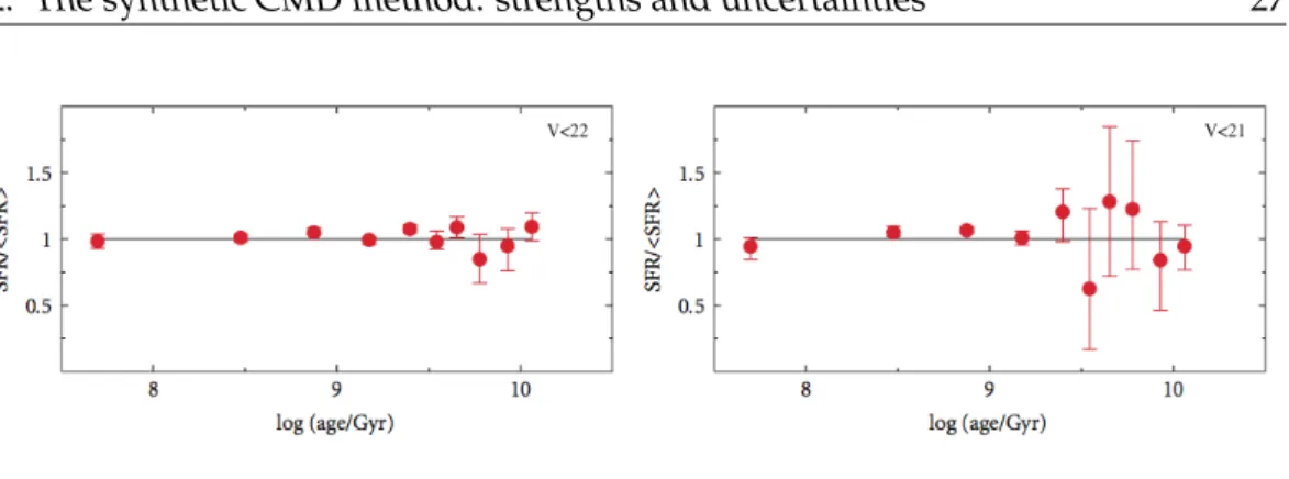
The first test they made is on the completeness limit, thus they performed the star formation recovery using only stars brighter than V = 21 and V = 22. The results are shown in Figure 2.6. As discussed before, deep CMDs allow to accurately derive the old star formation activity, while the quality already drops when the complete-ness limit is at V = 22. The larger error bars at old epochs reflect the fact that the only signature of the oldest activity comes from evolved stars, less frequent, and much more packed in the CMD than the corresponding MS stars. Rising the lim-iting magnitude at V = 21 further worsens the result, and the recovered SFH is a factor of 2 more uncertain for ages older than 1 2 Gyr.
Another tested parameter is the IMF. It is commonly assumed that the stellar IMF has a rather universal slope. Above 1 M the IMF is well approximated by a power law with a Salpeter-like exponent (Salpeter, 1955), while below 0.5 M it flattens. According to Kroupa (2001), the average IMF (as derived from local Milky Way star-counts and OB associations) is a three-part power law in the form ⇠(m) / m ↵, with exponent:
• ↵ = 1.3 ± 0.5 for 0.08 < m < 0.5 M , • ↵ = 2.3 ± 0.3 for 0.5 < m < 1 M , • ↵ = 2.3 ± 0.7 for m > 1 M .
Given the degeneracy condition that different combinations of IMF and SFH can equally match the present day mass function (the current distribution of stellar masses) of MS stars, it is interesting to evaluate how this impacts the possibility to infer the SFH. To quantify it, Cignoni and Tosi (2010) generated two populations with different IMF exponents (↵ = 2, and ↵ = 2.7), but performing the SFH search using always ↵ = 2.35.
As shown in Figure 2.7 the fit tends to over-estimate the SFR of any population whose IMF is actually steeper than the adopted one, and vice versa, for a flatter IMF. This solution is only the best solution in a parameter space where the IMF is fixed, and not necessarily has to be considered a good one: if the CMD of the recovered SFH is compared with the reference CMD, it is clear that the ratio between low- and
26 Chapter 2. From theory to practice high-mass stars is wrong. In other words, to figure out whether the “best” solution is actually acceptable, it is always crucial to compare all its CMD results with the observed one.
Another source of uncertainty is the percentage of stars in unresolved binary sys-tems and the relative mass ratio. The presence of a given percentage of not resolved binary systems affects the CMD morphology. To see if these effects can alter the re-covered information on the SFH, Cignoni and Tosi (2010) built fake populations us-ing different prescriptions for the binary population (10%, 20%, and 30% of binaries
FIGURE 2.5: Top panel. CMD of an artificial population of stars generated with constant SFR, Salpeter IMF, constant metallicity Z = 0.004, (m M )0 = 18.9, E(B V ) = 0.08, and HST/ACS photometric errors and completeness. Bottom panel. Input (solid black line) and recovered (red dots) SFH. See Figure 6 of Cignoni
2.2. The synthetic CMD method: strengths and uncertainties 27
FIGURE2.6: Effect of different completeness limits on the SFH recovery. Left panel. The SFH is recovered using only stars brighter than V = 22. In this case, most of the information is still retrieved. Right panel. The completeness limit is lowered at V = 21and, as expected, most of the old star formation (older than 1 Gyr) is much
more uncertain. See Figure 7 of Cignoni and Tosi (2010) for more details.
FIGURE 2.7: Effect of different IMF slopes. The SFH was recovered assuming
Salpeter’s IMF exponent (↵ = 2.35) for synthetic stellar populations actually gen-erated adopting different IMF (labeled in each panel) and a constant SFR. See
Fig-ure 8 of Cignoni and Tosi (2010) for more details.
with random mass ratio), but the SFH was searched ignoring any binary popula-tion (i.e., assuming only single stars). The adopted stellar models did not include binary evolution with mass exchange, thus each star in a double system is assumed to evolve as a single star.
Figure 2.8 shows the results, and a modest systematic effect is visible. This is because the stars in binary systems are brighter and redder than the average single star pop-ulation (Olsen,1999). For the recent SFH, this corresponds to moving lower MS stars from a star formation step to the contiguous older step: in this way, the most recent star formation step is emptied of stars, mimicking a lower activity. Intermediate SF epochs are progressively less affected, because some stars get in and some stars get out of the step bin. For the oldest epochs, the situation is opposite: the binary effect is to move stars toward younger bins.
The precise position of a star on the CMD depends on its chemical composition. The Zcontent mainly changes the radiative opacity and the CNO burning efficiency: the result of a decreasing Z for main sequence stars is to increase the surface temperature and the luminosity of the stars. This has two consequences of relevance for SFH studies: (a) metal poor stars have a shorter lifetime compared to the metal-rich ones
28 Chapter 2. From theory to practice
FIGURE2.8: Effect of unresolved binaries. Three fake populations are built with different percentage of binary stars (10%, 20%, and 30%). The SFH is recovered using only single stars. See Figure 9 of Cignoni and Tosi (2010) for more details.
2.2. The synthetic CMD method: strengths and uncertainties 29 (because overluminous and hotter), (b) a metal-poorer stellar population is bluer but can be mistaken for a younger but metal-richer population.
To test these effects, the first stars (ages older than 5 Gyr) in the reference fake popu-lation are built with a slightly different metallicity (Z = 0.002) than the younger ob-jects, which have the usual Z = 0.004. Then, the SFH is recovered adopting a model with constant Z = 0.004. The results are shown in Figure 2.9. Neglecting that the oldest population of our galaxy was slightly metal poorer produces systematic, non-negligible discrepancies in the recovered SFH. This is what is called age-metallicity degeneracy: to match the blue-shifted sequences of old metal poorer stars, the mod-els with wrong metallicity must be younger. Note that the overall trend of the young SFR is not significantly biased, while the old SFR is now significantly different.
FIGURE2.9: Sensitivity test to metallicity. The reference fake galaxy has a variable composition: Z = 0.004 for stars younger than 5 Gyr, Z = 0.002 for older stars. The red dots represent the SFR as recovered using a single metallicity, Z = 0.004,
for all epochs. See Figure 10 of Cignoni and Tosi (2010) for more details.
This result is a strong warning against any blind attempt to match the CMD with a single (average) metallicity, especially considering that many galaxies exhibit a pronounced age-metallicity relation.
During and at the end of their life, stars pollute the surrounding medium, so it is natural to expect that more recently formed stars have higher metallicity and helium abundance than those formed at earlier epochs. The progressive chemical evolution with time results from the combined contribution of stellar yields, gas infall and outflows, mixing among different regions of a galaxy. Observational studies have shown that several galaxies reveal a metallicity spread at each given age.
30 Chapter 2. From theory to practice
2.3 Matching the two worlds: SFERA
To explore the wide parameter space involved in the derivation of the SFHs, Michele Cignoni, at the INAF Bologna Observatory, has developed SFERA (Star Formation Evolution Recovery Algorithm) a hybrid-genetic algorithm that combines a classical genetic algorithm (Pikaia2, already implemented in IAC-pop, see Aparicio and Hi-dalgo,2009) with a local search (Simulated Annealing, as in, e.g., Cole et al.,2007). This allows to take advantage of the exploration ability of the former, which scans the parameters space in more points simultaneously and thus is not too sensitive to the initial conditions, and the capability of the latter of local exploration of the space and faster convergence. The proposed algorithm alternates two phases: the search for a quasi-global solution by the genetic algorithm and the local search by the other one, whose goal is to increase the solution accuracy (Cignoni et al.,2015).
For this thesis, we further developed the routines dedicated to the grid selection and reddening treatment, we improved the artificial star test technique and inserted the possibility of using different stellar models.
As shown in the scheme in Figure 2.10, the code requires the following input param-eters: stellar evolution library, IMF, binary fraction with secondary IMF, metallicity range. If information on the current metallicity of the analyzed galaxy (e.g. from spectroscopy of the H II regions) is available, in the youngest temporal bins the
metallicity is allowed to vary in a small range around this value, while the oldest bins have no constraints; this way, we don’t assume a priori an age-metallicity rela-tion nor the same metallicity for all the stars, and we can check whether we recover physically meaningful Z(t) relations.
From these inputs the code populates the isochrones in a chosen set of photometric bands via Monte Carlo extraction of stars (mass-age pairs) from the assumed IMF, with a constant SFR; each star will be alive (thus, visible on the synthetic CMD) or dead (thus, contributing only to the astrated total mass) according to its lifetime from the stellar evolution models. These “clean” models are then convolved with the photometric characteristics of the data, as described is Section 2.2.
The minimization of the residuals between data and models is implemented in SFERA taking into account the low number counts in some CMD cells, so we follow a Poissonian statistics, looking for the combination of BFs that minimizes a likelihood distance between models and data. This corresponds to the most likely SFH for these data, with an uncertainty given by the sum in quadrature of the statistical uncertainty (computed through a data bootstrap) and the systematic uncertainty (obtained by re-deriving the SFH with different age and CMD binnings, and using different sets of isochrones).
2Routine developed at the High Altitude Observatory and available in the public domain:http: