The 3D numerical simulation of near-source ground motion during the Marsica earthquake, central Italy, 100 years later

Submitted for publication to Soil Dynamics and Earthquake Engineering – January 27 2016

1

The 3D Numerical Simulation of Near-Source Ground Motion during

the Marsica Earthquake, Central Italy, 100 years later

R. Paolucci1, L. Evangelista2, I. Mazzieri3, E. Schiappapietra4

ABSTRACT

In this paper we show 3D physics-based numerical simulations of the devastating Marsica earthquake, Central Italy, occurred 100 years ago. The results provide a realistic estimation of the earthquake ground motion and fit reasonably well both the geodetic measurements of permanent ground settlement, and the observed macroseismic distribution of damage. In addition, these results provide a very useful benchmark to improve the current knowledge of near-source earthquake ground motion, including evaluation of the best distance metric to describe the spatial variability of the peak values of ground motion, the relative importance of fault normal vs fault parallel components, the conditions under which vertical ground motion may prevail, as well as the adequacy of 1D vs 3D modelling of site amplification effects.

1. Introduction

100 years ago, on January 13, 1915, at 6:52 local time, a catastrophic earthquake devastated Marsica, Southern Abruzzi, Central Italy, causing around 33,000 fatalities. Among the most important municipalities hit by the earthquake, the ruin of Avezzano was complete, with 10,700 fatalities, 95% of the total population [1]. A single reinforced concrete building in Avezzano, one of the very first ones at those times, withstood the earthquake and was later declared national monument. Unfortunately, since Italy was about to enter World War I, the government minimized the effects of the earthquake and denied the international support which was a key for the recovery after the Reggio-Messina catastrophe of December 28, 1908, only 4 years before. Therefore, the rescue operations were dramatically slow and some further 3,000 fatalities were estimated because of post-earthquake diseases.

The earthquake was felt up to several hundred km distance: for example, in Rome, about 80 km W of the epicentre, the IMCS intensity was estimated from VI to VII. A sketch of the MCS

intensities through the Southern Abruzzi region, together with the surface projection of the fault and the location of the instrumental epicentre is illustrated in Fig. 1.

The earthquake was originated by the Fucino fault system [2] consisting of an array of NW-SE striking normal faults, dipping mainly SW, which is also attributed to have generated the earthquake which severely affected Rome in 508 AD [3]. While clear evidence of the surface fault rupture was pointed out by the post-earthquake survey by Oddone [4], who followed the fault trace from SE to NW for about 33 km, there is no consensus on the epicentre location. As a

1

Professor, Dept. Civil and Environmental Engineering, Politecnico di Milano, Italy, roberto.paolucci@polimi.it

2

Researcher, Institute for Coastal Marine Environment (IAMC), National Research Council (CNR), Naples, Italy, lorenza.evangelista@cnr.it

3

Post-doc researcher, MOX - Laboratory for Modeling and Scientific Computing, Department of Mathematics, Politecnico di Milano, Milan, Italy, ilario.mazzieri@polimi.it

4

2

matter of fact, this is often reported, such as in [1], to be located at the center of the maximum intensity macroseismic area, roughly coinciding with the center of the Fucino basin. In addition, an instrumental determination was proposed by [5], and also reported by [6] in a special volume dedicated to the Marsica earthquake, based on the available seismometer recordings, which lead to the location 41.975 N – 13.605 E, which has been used in this paper and is shown in Fig. 1. Different determinations of the earthquake magnitude are also reported in the literature, and reviewed by [6], leading to Ms evaluations ranging from 6.6 to 7.0.

The presence of a prevailing normal faulting system bordering a tectonic basin is one of the key features of seismogenic activity in the Central-Southern Apennines, and poses the key problem of coupling the presence of the seismic fault with soft sedimentary basins, having relatively young age and large thickness, thus enhancing the hazard typical of near-source conditions. In this research, we have simulated near-source ground motion during the Marsica earthquake, taking advantage of the SPEED code, developed at Politecnico di Milano to perform 3D physics-based numerical simulations of seismic wave propagation. These include a kinematic model of the seismogenic fault rupture and a 3D model of the shallow crustal layers, including the complex geological irregularity of the Fucino basin.

Different objectives were pursued during this work, namely: (1) providing numerical results suitable to constrain the physical parameters of the earthquake, also by verifying the simulated permanent ground displacements against the vertical settlement estimated by post-earthquake geodetic measurements; (2) verifying possible conditions of directivity and interaction with the soft deposits of the Fucino basin, in order to explain the vast devastation in Avezzano, at the Northern edge of the basin, at some 20 km NW of the epicentre; (3) quantifying some relevant parameters of ground motion in near-source conditions, such as the ratio of strike fault normal (FN) vs fault parallel (FP) and the vertical vs horizontal components, as well as their spatial variability; (4) evaluating the best distance metric to model the peak values of ground motion in near-source conditions; (5) evaluating the adequacy of 1D modelling of site amplification effects in near-source.

2. Geological and Geotechnical Characterization

2.1 Geological framework and geotechnical characterization of Fucino basin

The Fucino basin is the most important intra-mountain depression of the Central Apennines, surrounded by high carbonate ridges of Meso-Cenozoic age. It covers an area of 900 km2, of which 200 km2 are an ancient lake, drained in 1875. The latter was the last proof of a long geologic evolution started in the Pliocene, during which the area was always lower than the surrounding Apennines, interested by uplift movements. The current geological setting of the Fucino basin, illustrated by the geological map and cross-section drawn in Fig. 2, results from a complex sequence of depositional events, due to erosion and tectonics.

The bedrock consists of Meso-Cenozoic carbonate, generally covered by terrigenous Neogene flysch deposits but also outcropping along the sides of the basin. The bottom of the basin was filled during the Quaternary with continental deposits of variable genesis and deposition age, resulting from lacustrine to subsequent alluvial sedimentations. In detail, the sedimentary sequences were divided [7] into:

3

- a Lower Unit (Plio-Pleistocene), outcropping on the North-eastern border of the basin, that mainly consists of breccias and alluvia, with subordinate lacustrine deposits;

- an Upper Unit (Upper Pleistocene-Holocene), made up of interdigitated lacustrine and alluvial deposits, that at the border of the depression heteropically evolves into alluvial fan deposits, which may even be coarse-grained.

Finally, the Quaternary sedimentary sequence is closed by thick lacustrine deposits in the center of the basin [8].

Fig. 1. IMCS distribution according to the Italian macroseismic database [9], including the epicenter and the surface projection of the fault adopted in this work.

This geomorphological setting is the result of a post-orogenic relaxing phase of the central part of Apennines, whose normal fault systems, with NW-SE and E-W-trending high-angle and S-SW-dipping, developed extensional basins along the south-western sector of the overthrust belt [10].

The complex geologic structure is characterized by the overlap, through two separate phases, of two semi-graben; the first one fully developed during the Pliocene, while the second one developed in the Plio-Pleistocene. In Fig. 2a, the isochron map in two-way time (TWT) of lacustrine deposits from seismic profiles is reported. The map shows the presence of a first sub-basin felt in the North sector near Avezzano with TWT equal to 250 ms and a second well defined depocentre near San Benedetto, the so-called Bacinetto, characterized by TWT of 900

4

ms. Assuming the P-wave velocity for bedrock VP = 2000 m/s [11], it is possible to derive that

the first sub-basin near Avezzano reaches a depth of 250 m, while the deeper one, corresponding to the Bacinetto, is characterized by a maximum depth of 900m.

Fig. 2. (a) Geological map and isochron contour map (interval 50 ms and 100 ms) of the alluvial and

lacustrine deposits (adapted from [7]); (b) Geological cross-section (from [11]), along the dashed line shown in the top.

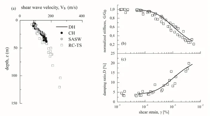
The lacustrine deposits, filling the latter sub-basin, was involved by an extensive geotechnical characterization activity in 1986 [12] to evaluate the dynamic subsoil properties. The specific investigations, planned for the geotechnical characterization, consisted of in situ, including Cross-Hole (CH), Down-Hole (DH), DMT and SASW, and a laboratory program consisting of resonant column (RC) and Torsional Shear (TS) tests. Fig. 3a shows the comparison of the in situ shear wave velocity (VS) profiles. The data from different sources show a good agreement within

the investigation depth and a significant increase of VS with depth. Since the in situ tests

5

thickness of lacustrine deposits was described by scaling the law of variation of the small strain shear stiffness (G0) with the mean effective stress (p') measured in RC-TS tests (Fig. 3a). To this

aim, the variation of G0 with p' observed in the RC-TS tests, was first expressed in terms of shear

wave velocity, VS (white squares in Fig. 3a), as a function of depth. The latter was related to p'

by assuming a coefficient of earth pressure at rest k0 = 0.8, that is the mean along the depth as

evaluated by DMT tests [12].

Fig. 3. (a) Comparison of shear wave velocity profiles obtained by DH, CH, SASW and RC-TS;

Normalised shear modulus (b) and damping ratio (c) versus shear strain from RC-TS tests.

The RC-TS tests confirmed the significant increase of VS along the thickness of lacustrine

deposits and allowed obtaining a shear wave velocity profile down to 100 m.

The non-linear behavior of lacustrine deposits was modeled based on the results of laboratory tests, reported in Fig. 3b-3c, in terms of variation of the normalized shear modulus, G/G0, and the

damping ratio, D, with the shear strain, γ. The variation of G/G0 vs γ is typical of medium-high

plasticity clay. The data is then interpolated with the Ramberg-Osgood law. Instead, the variation of damping ratio D (Fig. 3c) with shear strain γ was obtained by application of the Masing-modified criteria [13] to the modeled decay curve.

2.2 Construction of a numerical model

The numerical model of the Fucino basin extends over an area of 56x46x20 km3 (Fig. 4). It is built by assembling the topographic layer, obtained by a 250 m Digital Elevation Model, with the underlying layers describing the bedrock morphology as provided by seismic profiles [7]. The

6

fault geometry is also included into the model, as it will be discussed in the following section.

Fig. 4. 3D numerical domain, with a representative cross-section, transverse to the Apennine chain.

The bedrock morphology is derived by the interpretation of seismic profiles shown in Fig. 2. According to the geotechnical characterization described in the previous section, the filling deposits are assumed to behave as a non-linear visco-elastic medium, characterized by a unique profile of density (ρ), Poisson ratio (ν) and shear wave velocity (VS), as follows:

0.54 1530 0.1 ρ= ⋅ ⋅z (kg/m3) (1) 0.6 180 10 S V = + ⋅z and V =_P 10⋅V_S (m/s) (2) / 10 s Q = V (3)

The model of VS is in good agreement with those derived by [11] from experimental

measurement of resonance frequency by standard spectral ratio (SSR) and horizontal-vertical spectra ratio (HVSR) methods. The quality factor Q is derived directly by the VS values and is

assumed to be proportional to frequency as Q = Q0f, with Q0 set for the target value Q = VS/10,

specified at f =0.5 Hz.

It is worth highlighting that an outcropping bedrock is assumed outside the boundaries of the Fucino basin. Therefore, numerical results outside the Fucino basin are representative only of outcropping bedrock conditions and cannot be directly used to quantify ground motion in surrounding valleys, such as Valle del Liri, SW of the basin, which was also dramatically affected by the earthquake (see Fig. 1).

A crustal model is adopted based on [14]. It is characterized by five horizontal and parallel layers resting on a half-space at a depth of 20 km. In particular the VS values of the shallow layers have

been reduced with respect to those of [14], in agreement with the site investigations [15], in order to decrease the basin-to-rock impedance ratio. The properties of each layer are shown in Table 1.

7 Table 1

Horizontally stratified crustal model assumed for the 3D numerical simulations.

H (m) VS (m/s) VP (m) ρ (kg/m3) Q 500 1000 1800 2300 100 1000 1700 3160 2500 150 2000 2600 4830 2840 250 5000 3100 5760 2940 300 20000 3500 6510 3180 350

3. Kinematic modeling of the seismic source

There is a general consensus that the Marsica earthquake was generated along the Fucino system of normal faults [3], which borders on the Eastern side the Fucino basin, the strike of which is aligned along the Apennines chain. This indication is well constrained by different sources, such as by the post-earthquake survey of Oddone [4], who clearly witnessed the evidence of the line formed by the surface fault rupture, extending about 30 km from SE to NW, by the downward settlements of the 18 geodetic benchmarks (monumental statues) placed around the Fucino lake before drainage in 1875, on the hanging wall side of the rupture [16-18], and by the numerous paleoseismological studies in that area ([19], [2-3]).

The set of fault parameters considered in our numerical simulations is summarized in Table 2, while the slip distribution is illustrated in Fig. 5. We mainly based the geometric parameters (dimensions, position, strike, dip, rake) on Galadini (personal communication, 2015), the slip distribution on [16], and the epicentre on the instrumental location by [5]. By modulating the amplitude of slip distribution, we considered a range of MW from 6.7 to 7. The value MW 6.7

reported in Table 2 is the one for which the best agreement was obtained with the benchmark settlements, as discussed later.

4. Numerical modeling of seismic wave propagation by Spectral Elements

4.1 SPEED: Spectral Elements in Elastodynamics with Discontinuous Galerkin

SPEED is a certified numerical software (http://speed.mox.polimi.it) for 3D elastodynamics problems, that is specifically suited to study seismic wave propagation and dynamic soil-structure interaction problems in complex geological configurations. The code is jointly developed at MOX - Laboratory for Modeling and Scientific Computing of the Department of Mathematics and at the Department of Civil and Environmental Engineering of Politecnico di Milano. The SPEED kernel is based on a discontinuous version of the classical Spectral Element (SE) method, a non-conforming domain decomposition technique combining the flexibility of discontinuous Galerkin finite elements with the accuracy of spectral techniques. Based on the work of [20], the SE approximation described in [21] and [22] has been extended to address discontinuous discretizations.

8

Indeed, Discontinuous Galerkin Spectral Element (DGSE) approaches are shown to be able to capture local variations of the physical solutions while locally preserving the same accuracy of SE methods in term of dissipation and dispersion errors (see [20]). Moreover, DGSE methods can handle non-matching grids and different local approximation degrees making such schemes much more flexible than classical SE approaches from the mesh generation point of view (at price of an increased computational complexity). Finally, DGSE methods enjoy a high level of intrinsic parallelism, making such a discretization technique well suited for massively parallel computations [23].

Table 2.

Fault parameters adopted in this work.

Fault Parameters Present study Fault Geometry

Fault Origin FO (Lat, Lon) (42.15, 13.37)

Top Depth of Fault Hmin (km) 0.337

Length along Strike L (km) 41.6 Width along Dip W (km) 20

Epicenter (Lat, Lon) (41.97, 13.60) Focal Depth (km) 6.4 Strike (°) 127.8 Dip (°) 53.3 Seismic moment M0 (Nm) 1.25 10 19 Mw 6.7 Rise time τ (s) 0.70 Rupture Velocity VR (m/s) 0.85 VS Rake (°) 260

The present version of SPEED includes the possibility to treat seismic wave propagation in linear and non-linear visco-elastic heterogeneous soils, characterized either with frequency proportional quality factor [24], or frequency constant quality factor [25]. Paraxial boundary conditions [26] are introduced to reduce spurious reflections from outgoing waves inside the computational domain, while time integration can be performed either by the second order accurate explicit leap-frog scheme or the fourth order accurate explicit Runge-Kutta scheme (see [27]).

Recently, SPEED was successfully applied for the numerical simulation of near-source ground motion during the 2012 Po plain seismic sequence in Italy [28], for hazard assessment analysis in large urban areas for reinsurance evaluations as described in [23], as well as for city-site interaction problems and for the dynamic response of extended infrastructures [29].

9

4.2 Spectral Element model and numerical performance

The 3D computational domain used for the SPEED simulations was built based on data described in Sections 2 and 3, being a compromise between, on one side, the need to fit as closely as possible the available geological and geophysical information throughout a large spatial region, and, on the other side, to cast such information within a reasonably simple form apt to construct the computational model.

Considering a rule of thumb of 5 grid points per minimum wavelength for non-dispersive wave propagation in strongly heterogeneous media by the SE approach (cfr. [20]), and considering a maximum frequency fmax = 2 Hz, the model consists of 156.562 hexahedral elements, resulting

in 10.185.545 degrees of freedom, using a fourth order polynomial approximation degree. A conforming mesh was set up, having size ranging from a minimum of 200 m, within the quaternary basin, up to 440 m in the outcropping bedrock, and reaching 1250 m in the underlying layers, see Fig. 5a.

Fig. 5. (a) 3D computational mesh adopted for the numerical model along with the projection of the

seismic fault responsible of the January 13 1915 earthquake and buried topography, corresponding to Quaternary sediments in Fig. 2. (b) Assumed slip distribution to model the earthquake fault rupture, as described in Section 3.

A fault plane was introduced in the numerical model (Fig. 5b), complying with the geometric and kinematic features reported in Table 2. At each cell of the fault plane, a slip time history s(t) is prescribed in terms of an approximate step function:

( )

where erf (·) is the error function, τ = 0.7 s is rise time, t0 is the rupture time from the hypocentre to the cell, and the final slip s0 is mapped in Fig. 5. To enhance the high-frequency radiation, a

random variability of rise time and rake angle around their average value is considered, with

10

similar spatial correlation [30]. Moreover, to avoid the onset of very high velocity pulses due to super-shear effects, the rupture velocity has been bounded to VR = 0.85VS , being VS the shear

wave velocity at the corresponding source depth.

For the numerical simulations the time integration has been carried out with the explicit second order accurate leap-frog scheme, choosing a time step ∆t = 0.001 s for a total observation time T = 50 s. The simulations have been carried at the Idra cluster located at MOX-Laboratory for Modeling and Scientific Computing, Department of Mathematics, Politecnico di Milano (http://hpc.mox.polimi.it/hardware/) using 32 parallel CPUs, resulting in a total computation time of about 24 hours for a single simulation.

5. Discussion of results

5.1 Permanent vertical settlements

We have first verified the adequacy of the fault geometry and of the slip distribution model by comparing the simulated vertical displacements with the post-earthquake geodetic measurements performed by Loperfido [31] (values taken from [17]). In Fig. 6a, the map of permanent vertical ground displacements is reported, together with the location of geodetic benchmarks. The comparison is shown in Fig. 6b for two values of MW, obtained by changing the amplitude of slip

distribution. The best agreement was found for MW 6.7, compatible with the best solution of [18]

who found the minimum misfit with MW 6.6±0.1.

Fig. 6. (a) Map of permanent vertical displacements computed by SPEED for a simulated earthquake

magnitude Mw 6.7, with the slip distribution in Fig. 5. (b) Comparison of the historical values from geodetic measurements [31] (blue line), with the simulated permanent displacements obtained with Mw 6.7 (green line) and Mw 6.9 (red line).

As reported by [18], Loperfido himself underlined that some measurements might have been inaccurate, as benchmark 6, which was pulled off by the earthquake, and benchmark 11, lying on marshland and possibly subjected to additional ground settlements. It should be pointed out that

11

the numerical code is based on the assumption of elastic material behavior, so that it cannot model the sharp offset due to the fault rupture. Rather, a regular transition from negative to positive values of displacement is obtained, with very large, albeit elastic, ground strains.

5.2 Fault Normal and Fault Parallel components

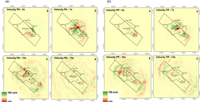
In Fig. 7, snapshots of horizontal ground velocity, rotated in the strike fault normal (FN) and fault parallel (FP) components, are shown. The amplification of motion due to basin effects is very clear. Also, it is worth to remark that, while in the initial phase of motion the FN component is prevailing, as it should be due to the normal faulting assumption (although a very small strike slip component is present, as shown by rake angle = 260°, see Table 2), the FP component becomes very clear inside the basin at about 7 s. This is mainly associated to Rayleigh waves, generated inside the basin, propagating in the NW direction towards Avezzano.

Fig. 7. Snapshots of the computed velocity field at different time instants T = 5, 7, 10, 15 s. (a) Fault

Normal (FN) component. (b) Fault Parallel (FP) component.

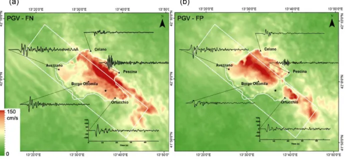
The peak ground velocity (PGV) maps of the FN and FP components, together with the corresponding velocity records, are illustrated in Fig. 8. Here, the observed variability of ground motion is striking, with different features observed on the footwall (Pescina and Celano) and on the hanging wall of the fault (Ortucchio, Borgo8000, Avezzano), probably related to the coupling of different soil conditions and different location with respect to the fault plane. Duration of the strongest portion of ground motion is about 5 s, in very good agreement with the reports of the survivors [4].

It is also worth to remark that the largest PGV values occur close to the edge of the surface projection of the fault plane. However, these values are likely overestimated by our numerical

12

simulations, because the energy dissipation due to the surface fault rupture is not accounted for, although a moderate nonlinear response is considered through a nonlinear elastic model following the curves in Fig. 3b. To underline the difficulty in predicting peak ground motion values in the proximity of the fault, it is worth to remark that the available records during the MW

6.7 Fukushima Hamadoori, Japan, normal faulting earthquake on April 12, 2011 [32], therefore in similar conditions as in our study, have shown PGV values larger by a factor ranging from 1.4 to 1.8 than the predicted ones by ground motion prediction equations (GMPE).

Fig. 8. PGV map for the FN (a) and FP (b) components, together with the corresponding velocity time

histories at selected sites (Avezzano, Ortucchio, Pescina, Celano, Borgo Ottomila).

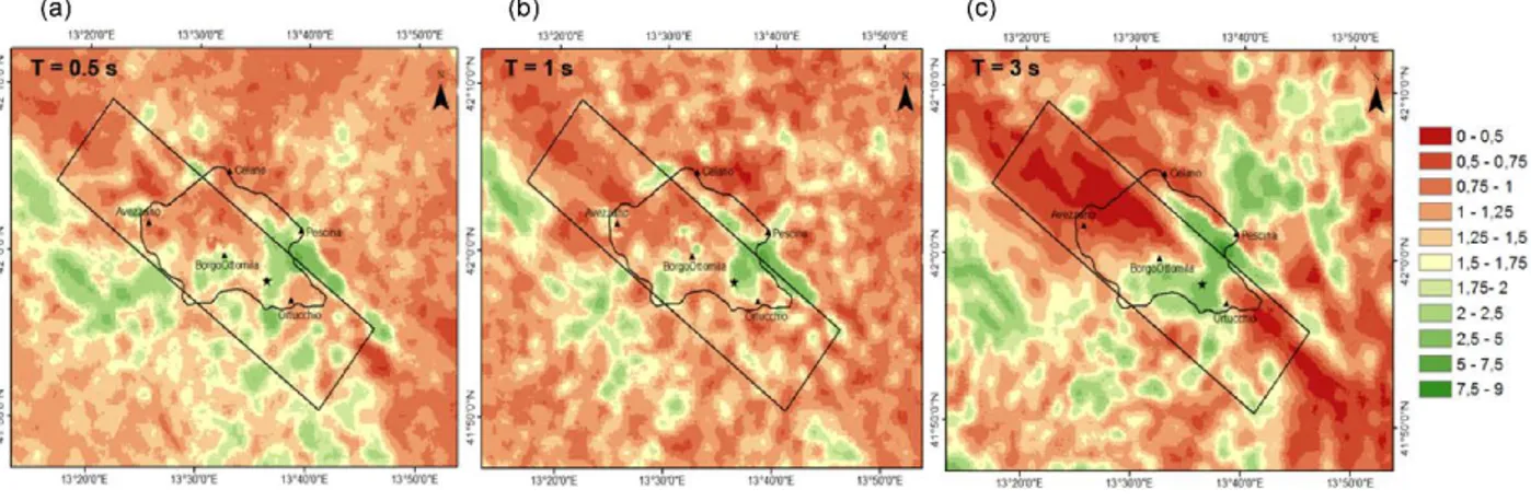
Next, we show in Fig. 9 the spatial distribution of response spectral ratios (5% damped) of the FN vs FP components of motion, for vibration periods T = 0.5 s, 1 s, 3 s. It can be seen that this ratio is by far larger than 1 in the proximity of the surface fault rupture, as expected for a normal fault. Moving away from the largest asperities of the fault rupture, this ratio decreases to values typically ranging between 1 and 1.5. It is worth noting that, as seen from the right hand side plot on Fig. 9, the FP component tend to dominate at long periods (T = 3 s) close to the NW side of the basin, probably due to the dominance of Rayleigh waves propagating in that direction, as noted previously.

It is also interesting to make a further check with the observation, made by Oddone [4], of the prevailing “azimuth of shaking”, i.e., the direction of the strongest shaking based on the observed damage on buildings. One century ago, this was one of the most common ways to estimate the prevailing direction of strong ground motion. Such directions were depicted by Oddone as arrows in the isoseismal plot, based on the original Mercalli scale, that he constructed after the earthquake (Fig. 10). We have highlighted in the same figure the arrows at the localities of Ortucchio, Avezzano and Celano, and superimposed the orbits of ground motion in the horizontal plane. It can be seen that, while in Ortucchio this was recognized to be roughly in the

13

FN direction, as also predicted by our simulations, both in Avezzano and Celano the evidence of a roughly FP prevailing direction was found by [4], again in reasonably good agreement with the numerical simulations.

Fig. 9. Spatial distribution of the ratio between FN and FP component of 5% damped response

acceleration spectrum for T = 0.5 s (a), 1 s (b), 3 s (c).

Fig. 10. In the background (Fig. center), the isoseismal map compiled by [4] after the earthquake,

together with the arrows denoting the prevailing “azimuth of shaking”. Superimposed are the plots of the orbits of ground motion in the horizontal plane, computed by the numerical simulations, at the sites of Avezzano, Ortucchio and Celano.

14

Different studies based on near fault records (see e.g., [33-34]) highlighted that the ratio of vertical to horizontal response spectra (V/H) is strongly dependent on period, with V/H values that may be substantially larger than 1 at short periods (T < 0.2 s) but that typically fall to about 0.5-0.6 at longer periods. We have explored the vertical components of ground motion from our simulations, to check whether a similar trend is found, although it should be remarked that the computational frequency limit of our simulations is about 2 Hz.

First, we have plotted in Fig. 11 the vertical PGV map, with a sample of vertical velocity time histories, similarly to Fig. 8, showing consistently large values throughout the basin, especially close to the fault rupture, where the values experienced are similar to the horizontal ones, shown in Fig. 8. Such large impact of the vertical components may be explained in terms of the normal tectonic movement with a major vertical component involving practically the whole Fucino basin, as shown in Fig. 6.

Fig. 11. PGV map for the Z component, in the same format as Fig. 8.

We have further explored in Fig. 12 the spatial variability of the ratio of vertical component with respect to the geometric mean of the horizontal ones (FN, FP) as a function of period, with reference to T = 0.5s, 1s, and 3s. Probably, the most striking feature of such spatial distribution is the opposite trend at short and long periods. As a matter of fact, in the first case, the vertical component tends to dominate, while the opposite is for the second case. A hint to understand such feature may be found in the horizontal-to-vertical spectral ratios obtained by [11] (a sample of them is shown in Fig. 12b), where, within the basin, peaks are typically found in the frequency range from 0.2 to 0.4 Hz, but, correspondingly, troughs are present in the range from 2 to 3 Hz. Therefore, it may be argued that, in the 2-3 Hz frequency range, the Fucino basin experiences site amplification effects on the vertical component, i.e., associated to possible 3D resonance of the longitudinal waves. This would be one of the few cases where the vertical component of ground motion dominates in a period range beyond 0.2 s, involving a major impact on engineering structures.

15

Fig. 12. Spatial distribution of the ratio between Z and the geometric mean of FN and FP components of

5% damped response acceleration spectrum for T = 0.5 s (a), 1 s (b), 3 s (c). In the (b) panel, the horizontal-to-vertical spectral ratios at two locations of the array investigated by [11] are shown.

5.4 Comparison with GMPEs and considerations on the optimum distance metric in near-source

Comparison of our results with GMPEs is very instructive, not only in terms of peak values of motion, but also in terms of the corresponding spatial distribution. In Fig. 13, such a comparison is shown with the GMPE proposed by [35] based on Italian records (mostly from normal fault earthquakes). The geometric mean of the horizontal components is considered. The GMPE is found to underpredict the simulated values by a factor ranging from 2 to 4 in the vicinity of the source and especially for rock conditions.

Also, it is very clear that the adopted distance metric by [35], i.e., the Joyner-Boore distance (RJB) from the surface projection of the fault, is not fit to properly describe the spatial

distribution of ground motion in near-source conditions. As a matter of fact, by using the RJB

metric, all points on the surface fault projection are assigned the same peak value, irrespective of their actual position with respect to the fault rupture. This turns out to play a major role for those faults, either normal or reverse, with medium-to-low dip angles, for which a large surface projection of the fault is expected with a corresponding large variability of ground motion throughout that surface.

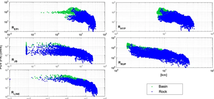
To explore this subject, we have studied the spatial variability of simulated ground motion considering different distance metrics, namely: RJB (Joyner and Boore), REPI (epicentral), RHYP

(hypocentral), RRUP (distance from the fault rupture). In addition to these classical distance

metrics, we have also proposed the metric RLINE, that is the distance from the surface fault

projection of the segment at the top edge of the fault. The actual position and length of the segment is set by projecting the hypocenter along the edge, and by considering it as the center of a segment of length given by the Wells and Coppersmith scaling relationships [36]. The resulting segment is shown by a red line on the right hand side map of Fig. 13.

16

Fig. 13. Map of the computed Peak Ground Velocity (PGV). Geometric mean of the horizontal

components obtained by SPEED (la) and by GMPE proposed by [35], (b).

Considering results in Fig. 14, for receivers up to about 40 km distance, the following comments can be made on the application of the different distance metrics:

- REPI: the scatter of results is very high and, more important, there is no tendency of decreasing

amplitude with distance, since the epicenter lies away from the area of largest amplitude;

- RHYP: the limitation is similar as with REPI, with a scatter at short distances exceeding one order

of magnitude;

- RJB: a large number of points in this case lies at RJB=0, that was set to a default value of 50 m

for representation in a log scale. A similar large scatter as for RHYP is found;

- RRUP: a correct decrease of amplitude with distance can be found, with a lower scatter of

results with respect to the previous cases. This may be considered as the best among the “classical” distance metrics typically used in the GMPEs to predict near-source ground motion; - RLINE: at short distance, the scatter is significantly reduced, while, at large distance, the scatter

is similar to the other cases.

We can conclude that, to improve the accuracy of prediction of ground motion in near-source conditions, especially for large earthquakes, the distance from the fault rupture plane (RRUP) is by

far the best metric among the classical ones used for GMPEs. However, the maps of PGV from numerical simulations, as well as the analysis of spatial variability from physics-based simulated ground motions, including also the recent experience with the May 29 2012 Po plain earthquake [28, 37], suggest that the best performance is obtained through the RLINE distance, that has also

17

Fig. 14. Variability of PGV (FN component) with respect to different distance metrics. Values are expressed in cm/s.

5.5 Evidence of 3D site effects in the basin amplification of seismic waves

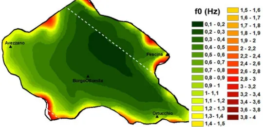
We have explored the characteristics of the spatial variability of site amplification within the Fucino basin by first computing the 1D natural frequency f0=Vs/4H, where H is the local

thickness and Vs the average shear wave velocity to the bedrock. The resulting map of f0 is

shown in Fig. 15, and clearly portrays the low values of f0 , typically ranging from 0.2 to 0.8 Hz

in the inner part of the basin, related to coupling low values of Vs to large sediment thickness.

If the response of the Fucino basin were dominated by 1D amplification effects, we should expect that the response spectral ordinates at given locations be larger at periods close to T=1/f0.

To verify this argument, we have plotted in Fig. 16 the map of residuals ε=log10(Sasim(R,T)/Saavg(R,T)), where Saavg(R,T) is the average simulated spectral ordinate at

period T and at distance R=RLINE, either within the basin or on rock, and Sasim(R,T) is the

corresponding value simulated at the specific location (geometric average of the horizontal components). Therefore, a positive value of ε means that the local site amplification at period T and distance R is larger than the average at the corresponding period and distance.

According to expectations from 1D modelling, these maps should roughly follow the spatial pattern of f0 in Fig. 15. However, the pictures in Fig. 16 portray a much more complex feature of

site amplification, with a broadband amplification in most sites within the inner portion of the basin (see e.g. Borgo Ottomila) and an irregular pattern at the edges. Consider for example the site of Avezzano, the main locality of Marsica, which was literarily devastated by the earthquake. In this case the residuals are positive both at short and long periods, probably related to the unlucky combination of 1D response at T = 1s with the propagation of long period surface waves towards the NW edge of the basin (see the plot for T=3s, Fig. 16c), which caused a dramatic broadband amplification of ground motion.

18

We can conclude that, in a near-source environment such as studied in this work, the features of site amplification may be much more complex than predicted by classical 1D approaches, as also shown in [38] in a similar geological framework in Central Italy, and that they should be more properly evaluated with additional consideration of the basin and fault geometry and of the kinematic of slip along the fault.

Fig. 15. Map of 1D natural frequency of vibration f0 of the Fucino basin.

Fig. 16. Map of residuals ε=log10(Sasim(R,T)/Saavg(R,T)), where Saavg(R,T) is the average simulated

spectral ordinate at period T and at distance R=RLINE, either within the basin or on rock, and Sasim(R,T) is the corresponding value simulated at the specific location. Three values of period are considered: T= 0.5 s (a), 1 s (b), 3 s (c).

6. Conclusions

This paper presented an overview of results of the 3D physics-based numerical simulations of the 1915 Marsica earthquake, which devastated Avezzano and surrounding villages, causing more than 33,000 fatalities. Results matched reasonably well some post-earthquake observations, such as the geodetic measurements of co-seismic vertical ground displacements, found to be consistent with a MW 6.7 earthquake magnitude, and the estimated prevailing directions of

19

shaking. Furthermore, they provided a realistic picture of earthquake ground motion in a condition, quite common in Central Apennines, where there may be a strong interaction of near-source conditions with the complex geology associated to the presence, within an extensional environment, of shallow tectonic basins with relatively soft-soil sediments.

A huge variability of earthquake ground motion within such a complex geological and tectonic configuration, both in terms of amplitude and prevailing features, was highlighted by this study, in line with the report of Oddone [4], who, in his strikingly in-depth survey of the consequences of the earthquake based on the failures of structures and interviews to survivors, found clear evidence and witnesses of “all imaginable types of motion”, from vertical, to horizontal, to rocking. A complexity hard to be predicted by standard engineering tools based on 1D shear wave propagation, such as demonstrated by the features of ground motion amplification and of the spatial distribution of the fault normal, fault parallel and vertical components.

In such complex near-source conditions, recent GMPEs may lead to underestimations of the earthquake ground motion amplitude, since they are rather poorly constrained because of scarcity of records. Furthermore, a careful choice should be made in terms of distance metric: among the classical metrics, RRUP turns out to be the best one, but the metric RLINE, introduced in this work,

provides better performance than RRUP for the normal fault condition examined in this study.

We can finally conclude that the numerical approaches and computational tools for 3D physics-based simulations are becoming more and more suitable to provide realistic ground shaking scenarios of past and future earthquakes, and are expected to provide in the next future an effective support to real records, to improve reliability of predicting tools of earthquake ground motions and seismic hazard evaluations.

Acknowledgments

This work was stimulated by the invitation received by the first author from Fabrizio Galadini, INGV, to present a lecture at the conference in Avezzano to commemorate the centennial from the earthquake. Fabrizio Galadini and Gianluca Valensise, INGV, provided useful comments and research material that was used to better constrain the numerical model. Funding from the DPC-RELUIS Project RS2, on Numerical simulations and near-source effects, is also gratefully acknowledged. Ilario Mazzieri was partially supported by the research grant no. 2015-0182 “PolyNum: Polyhedral numerical methods for partial differential equations” funded by Fondazione Cariplo and Regione Lombardia.

References

[1] Guidoboni E, Ferrari G, Mariotti D, Comastri A, Tarabusi G, Valensise G. CFTI4Med, Catalogue of Strong Earthquakes in Italy (461 B.C.-1997) and Mediterranean Area (760 B.C.-1500). INGV-SGA 2007. Available at http://storing.ingv.it/cfti4med/ (Last access: May 2015).

[2] Galadini F, Galli P. The Holocene paleoearthquakes on the 1915 Avezzano earthquake faults (central Italy): Implications for active tectonics in Central Apennines. Tectonophysics 1999; 308: 143-170. [3] Galli P, Messina P, Giaccio B, Peronace E, Quadrio B. Early Pleistocene to late Holocene activity of the

20

[4] Oddone E. Gli elementi fisici del grande terremoto marsicano fucense del 13 Gennaio 1915. Bollettino della Società Sismologica Italiana 1915; 29: 71-215 [in italian].

[5] Basili A, Valensise G. Contributo alla caratterizzazione della sismicità dell'area marsicano-fucense. in Proc. II Workshop on “Aree Sismogenetiche e Rischio Sismico in Italia”, E. Boschi and M. Dragoni (eds) Erice 1986; 197-214 [in italian].

[6] Favali P and Frugoni F. Revisione critica dei parametri fisici del terremoto. In: "13 gennaio 1915. Il terremoto nella Marsica” a cura di S. Castenetto e F. Galadini 1999; 273-282 [in italian].

[7] Cavinato GP, Carusi C, Dall’Asta M, Miccadei E, Piacentini T. Sedimentary and tectonic evolution of Plio-Pleistocene alluvial and lacustrine deposits of Fucino basin (Central Italy). Sedimentary Geology 2002; 148: 29-59.

[8] Giraudi C. Evoluzione geologica tardo pleistocenica ed olocenica della Piana del Fucino e dei versanti adiacenti: analisi di nuovi dati stratigrafi ci e radiometrici e ricostruzione delle variazioni ambientali. In 13 Gennaio 1915. Il terremoto della Marsica (a cura di Castenetto S. e Galadini F.). C.N.R., Serv. Sis. Naz., Ist. Poligr. Stat. Roma 1999; 183-197 [in italian].

[9] Locati M, Camassi R, Stucchi M. DBMI11, la versione 2011 del Database Macrosismico Italiano 2011. Milano, Bologna. Available at http://emidius.mi.ingv.it/DBMI11. DOI: 10.6092/INGV.IT-DBMI11. [10] Cavinato GP, De Celles PG. Extensional basins in the tectonically bimodal central Apennines

fold-thrust belt, Italy: response to corner flow above a subducting slab in retrograde motion. Geology 1999; 27 (10): 955-958.

[11] Cara F, Di Giulio G, Cavinato GP, Famiani, Milana G. Seismic characterization and monitoring of Fucino Basin (Central Italy). Bull. Earthquake Eng 2011; 9:1961-1985.

[12] Pane V, Burghignoli A. Determinazione in laboratorio delle caratteristiche dinamiche dell’argilla del Fucino. CNR Atti del Convegno del Gruppo Nazionale di Coordinamento per gli Studi di Ingegneria Geotecnica, Monselice 1988; 1:115-139 [in italian].

[13] Hardin BO, Drnevich VP. Shear modulus and damping in soils: Design equations and curves. Journal of Soil Mechanics and Foundation Division 1972; 98:667-692

[14] Ameri G, Gallovic F, Pacor F. Complexity of the Mw 6.3 2009 L'Aquila (central Italy) earthquake: 2. Broadband strong motion modeling. Journal of Geophysical Research 2012; 117, B04308.

[15] Working Group MS–AQ. Microzonazione sismica per la ricostruzione dell’area aquilana vol. 3 and Cd-rom. L’Aquila: Regione Abruzzo – Dipartimento della Protezione Civile 2010.

[16] Ward SN, Valensise G. Fault parameters and slip distribution of the 1915 Avezzano, Italy, earthquake derived from geodetic observations. Bulletin of the Seismological Society of America 1989; 79: 690– 710.

[17] Berardi R, Mendez A, Mucciarelli M, Pacor F, Longhi G, Petrungaro C. On the modelling of strong motion parameters an correlation with historical macroseismic data: an application to the 1915 Avezzano earthquake. Annali di Geofisica 1995; 38: 851-866.

[18] Amoruso A, Crescentini L, Scarpa R. Inversion of source parameters from near and far-field observations: an application to the 1915 Fucino earthquake, Central Apennines, Italy. Journal of Geophysical Research 1998; 103(B12): 29,989-29,999.

[19] Galadini F, Galli P, Giraudi C. Geological investigations of Italian earthquakes: new paleoseismological data from the Fucino plain (Central Italy). Journal of Geodynamics 1997; 24:87-103.

[20] Antonietti PF, Mazzieri I, Quarteroni A, Rapetti F. Non-conforming high order approximations of the elastodynamics equation. Computer Methods in Applied Mechanics and Engineering 2012; 209-212: 212 – 238.

[21] Faccioli E, Maggio F, Paolucci R, Quarteroni A. 2D and 3D elastic wave propagation by a pseudo-spectral domain decomposition method. Journal of Seismology 1997; 1(3): 237–251.

21

[22] Komatitsch D and Tromp J. Introduction to the spectral-element method for 3-D seismic wave propagation. Geophysical Journal International 1999; 139(3): 806–822.

[23] Paolucci R, Mazzieri I, Smerzini C, Stupazzini M. Physics-based earthquake ground shaking scenarios in large urban areas. in Perspectives on European Earthquake Engineering and Seismology, Geotechnical, Geological and Earthquake Engineering ed. Ansal, A., Springer 2014; 34: 10.

[24] Stupazzini M, Paolucci R, Igel H. Near-fault earthquake ground-motion simulation in the Grenoble valley by a high-performance spectral element code. Bulletin of the Seismological Society of America 2009; 99(1): 286–301.

[25] Moczo P, Kristek J, Galis M. The Finite-Difference Modelling of Earthquake Motions: Waves and Ruptures. Cambridge University Press 2014.

[26] Stacey R. Improved transparent boundary formulations for the elastic-wave equation. Bulletin of the Seismological Society of America, 1988; 78(6): 2089–2097.

[27] Butcher JC. Numerical Methods for Ordinary Differential Equations, 2nd Edition,Wiley, 2008. [28] Paolucci R, Mazzieri I, Smerzini C. Anatomy of strong ground motion: near-source records and 3D

physics-based numerical simulations of the Mw 6.0 May 29 2012 Po Plain earthquake, Italy. Geophysical Journal International, 2015; 203: 2001–2020.

[29] Mazzieri I, Stupazzini M, Guidotti R, Smerzini C. SPEED: SPectral Elements in Elastodynamics with Discontinuous Galerkin: a non-conforming approach for 3D multi-scale problems. International Journal for Numerical Methods in Engineering 2013; 95(12): 991–1010.

[30] Smerzini C, Villani M. Broadband Numerical Simulations in Complex Near-Field Geological Configurations: The Case of the 2009 Mw 6.3 L’Aquila Earthquake. Bulletin of the Seismological Society of America 2012; 102: 2436–2451.

[31] Loperfido A. Indagini astronomico-geodetiche relative al fenomeno sismico della Marsica. Atti Minist. Lavori Pubblici, Florence, Italy 1919; 95 pp. [in italian].

[32] Anderson JG, Kawase H, Biasi GP, Brune JN, Aoi S. Ground Motions in the Fukushima Hamadoori, Japan, Normal-Faulting Earthquake. Bulletin of the Seismological Society of America 2013; 103: 1935–1951.

[33] Gülerce Z. and N.A. Abrahamson. Site-Specific Design Spectra for Vertical Ground Motion. Earthquake Spectra 2011; 27: 1023–1047.

[34] Ambraseys, N. N., and Douglas, J. Near field horizontal and vertical earthquake ground motions. Soil Dynamics and Earthquake Engineering 2003; 23: 1–18.

[35] Bindi D, Pacor F, Luzi L, Puglia R, Massa M, Ameri G, Paolucci R. Ground motion prediction equations derived from the Italian strong motion database. Bull Earthquake Eng. 2011; 9:1899–1920. [36] Wells DL, Coppersmith KJ. New Empirical Relationships among Magnitude, Rupture Length,

Rupture Width, Rupture Area, and Surface Displacement. Bulletin of the Seismological Society of America 1994; 84: 974–1002.

[37] Hashemi K., Mazzieri I, Paolucci R, Smerzini C. Spatial Variability of Near-Source Seismic Ground Motion with respect to different Distance Metrics. 7th Int. Conf. on Seismology and Earthquake Engineering, Tehran, 2015, Paper n. 770-SM.

[38] Smerzini C, Paolucci R, Stupazzini M. Comparison of 3D, 2D and 1D numerical approaches to predict long period earthquake ground motion in the Gubbio plain, Central Italy. Bulletin of Earthquake Engineering, 2011, 9:2007–2029.