Cost efficiency of Italian Commercial Banks:
a Stochastic Frontier analysis.
Alessio Fontani
1, Luca Vitali
2,1CR Firenze and Luiss – Guido Carli Via Bufalini, 6 - 50122 Firenze e-mail: [email protected] 2University of Rome Tor Vergata Via Bernardino Alimena, 5 - 00173 Roma e-mail: [email protected]
Copyright © 2013 Horizon Research Publishing All rights reserved.
Abstract
During 90’s, the Italian banking system faced anew competitive environment both widening the dimensional scale and pursuing a rationalization process. Some insights could be drawn through efficiency analysis by estimation of a stochastic cost frontier for the period 1993-2004. Benchmark analysis not only highlights the contribution of the main factors that affect efficiency, but also allows evaluation of efficiency dynamics through time, determining the existence of technical progress and scale economies. However, such measure is significant if the sample of firms is homogeneous hence, accounting for heterogeneity of the units involved is then a goal of our analysis.
Keywords
Italian banks, Stochastic Frontier, CostFunction, Technical Progress, Heterogeneity
1. Introduction
At the beginning of 90’s, Italy adopted the Second EEC Banking Directive (89/646/EEC) on the coordination of laws, regulations and administrative provisions relating to the taking up and pursuit of the business of credit institutions. It represented the main step towards deregulation and harmonization of operational standards and practices, aimed at the creation of the European Common Banking Market. Until 80’s, Italian credit market was highly regulated, with portfolio constraints, credit constraints, limits to foreign currencies position-keeping and trading, high reserve requirements, restrictions to new branches in the national territory. Deregulation allowed the banking system to meet the requirements connected to the innovation process of financial institution, the development of IT-based production processes, the market globalization and the competition of specialized intermediaries. Further,
the prevailing public property of the control rights was an issue. The Government’s choice to privatize during 90’s was simply down to the need to raise capital, due to Maastricht Treaty criteria on public deficit to GDP and debt level to GDP. Subsequently, once the major banks were privatized, it became obvious that greater efficiency and profitability were necessary conditions to become more competitive in a larger European Union. So, the subsequent banking system reform process aimed at several goals: higher competition in the markets and consolidation of the whole sector while fostering the privatization process. These targets turns out only partially achieved: at first, one of the main shareholders of commercial banks are the “Fondazioni Bancarie” (Banking Foundations), a public (local or central state) agent which increased the degree of ownership concentration; secondly the large diffusion of hybrid subjects, like the Cooperative Banks and Mutual Banks (Banche Popolari and Banche di Credito
Cooperativo) where voting stocks are limited, thus creating
some distortion in a competitive environment. However, after 1990, the banking system privileged the rationalization of productive processes and ownership structure, usually increasing the dimensions, through merger and acquisition (M&A) operations, thanks also to low interest rates (leverage), that substantially affected the ownership structure, the degree of sector concentration, the geographical coverage and the (increased) number of branches. The final outcome will be a progressive change of the banking model. The process of concentration of the Italian banking system during 90’s affected nearly half of the whole sector, in terms of asset values1, and involved a significant reduction of the number of banks, operating in Italy. Italian banking groups showed similar dynamics, with a reduction (around 10%) of the number of subjects operating in Italy.
After 2000, only a small number of M&A operations were conducted on the domestic market: 37% of total asset was acquired by Italian banks between 1996 and 2000, 9% from 2001 to 2004. Therefore the weight of foreign acquisitions has progressively grown. Despite the M&A process, Italy still has a comparatively higher number of banks than France, Germany and Spain. However, such reduction in the number of banks does not imply necessarily benefits in terms of efficiency of operating units, neither less degree of competition, which stems from the distribution of branches, the development of alternative channels of distribution, especially in innovative sectors (such as asset management and structured finance). The considerable increase of the number of branches and the huge decline in the number of employees led to a sizable reduction of the labour cost (in real terms) in connection with the number of workers and of the cost-income ratio (total costs/overall business margin). Beside the cuts in total expenditures and the labour input rationalization, credit quality showed major improvements, with a considerable reduction, from 1997 onwards, of the non-performing loans (NPL) to total loans ratio. However, it should be stressed that, in 2001-2003, contraction of NPL has to be ascribed to an increase of securitization, particularly for large banks. Securitization allows only a partial risk reduction (in fact, the junior class - the speculative grade component of the ABS - was taken up by originator, while the Investment Grade ones took place at institutional investors), although the meaningful retrenchment of doubtful loans substantially contributed to reduce credit risk exposure. Thanks to securitization banks have met three results: a sharp reduction of NPL; a lower degree of exposure to credit risk of banking book; the release of free capital, which naturally increases the operating ability of credit institutions. Moreover, we have to remark the continuous improvement of capital adequacy, the strict control of the solvency ratio and the most efficient use of capital. After 2000’s IT bubble, more efficient and liquid financial markets, together with more effective risk attitude of the investors enabled credit institutions to improve their capital conditions, both with equities and subordinated debt; at present, supervisory capital closely meets Basel requirements, while there’s further room for systemic consolidation. Our data turns out rather homogenous. The size of production processes shows a stable and positive relation with costs and outputs: the correlation coefficients between the size variable (number of branches) and variables representing costs and outputs are next to 0,8.
So far, the empirical literature related to the Italian experience provided not always unambiguous results on the extent of product mix efficiency of the Italian banking system. Resti (2000), Focarelli et al. (1999) Girardone, Molyneux and Gardener (2004) point out that the mean level of cost inefficiency of Italian banks places between 13% and 15%, with a slight trend towards reduction over time. Evidence from Casu and Girardone (2007) confirms
that average overall efficiency score, in 2005 vary between 62.04% in DEA estimations and 80.47% (down from 84.13% in 2000) in SFA estimations.
Drummond, Maechler and Marcelino (2007) assess the degree of banking competition and efficiency in Italy. They find competition in the Italian banking sector has intensified in loan and deposit markets in recent years, but banks still operate in a high-cost, high-income system, and efficiency gains have yet to fully materialize. Persistently high operating profits, coupled with high revenues and/or high costs, are frequently associated with non competitive behavior. The pricing data suggest relatively high costs of banking.
In addition, many of these authors find important economies of scale; the more efficient credit institutions are placed in the northern part of the country, while dimensional scale is less significant.
This paper aims at investigating the performance of the Italian banking system from 1993 to 2004, determining the contribution of the main factors that characterize banks efficiency. Our analytical instrument is a stochastic cost frontier, which allows us to determine both a measure of technical efficiency and a ranking of productive units (based on the distance from the production contour), by comparing each unit with the case of full efficiency. The dynamic evolution of efficiency through time is also tested as well as the presence of technical progress and economies of scale. The specification of a cost function shared by the whole banking sector requires input and output indicators common to all firms (since multifunctional groups accede to the same technology, sharing the same factors), in order to obtain a meaningful benchmark; further, we include credit quality and riskiness indicators to account for the pronounced variations in credit assessment and performance and the development of new business models, which could affect the efficiency levels.
Deviations from the optimal path can be ascribed to inefficient input mix chosen by the management or to exogenous factors (random disturbances). But when panel data are non-homogeneous, firms can turn out to be simply different because of their size, their geographical position, their branch dispersion and their main business activity. Moreover, we provide further contribution to efficiency assessment, allowing for the influence of environmental heterogeneity on performances of Italian banking institutions. The paper is organized as follows. In chapter 2 we illustrate the methodology, data and estimation results. Chapter 3 shows panel estimates and heterogeneity effects on efficiency. Chapter 4 describes the hypothesis of time variability of the efficiency measure. Conclusions follow.
2. Methodology, data and estimation
results
The development of an efficiency measure, based on a production or cost frontier, obtained by DEA non
parametric technique, has been developed starting from the initial contribution of Charnes, Cooper and Rhodes (1978). The DEA approach, although more flexible, with no a priori constraints on data, does not discriminate among inefficiency and random disturbances, as any deviation from the deterministic frontier is interpreted as inefficiency, with no regard for other elements (as data measurement errors for instance). Alternatively, the parametric methodology of Stochastic Frontier Analysis (SFA), introduced by Aigner, Lovell and Schmidt (1977) and Meeusen and Van den Broeck (1977) and extended by Kumbhakar and Knox Lovell (2000) leads to a (stochastic) best-practice frontier, by comparison of performances of all units of the economic system; such methodology allows discrimination between the effect caused by stochastic disturbances or by technical inefficiency, which can simultaneously characterize the deviations from the best-practice frontier. Nonetheless, such parametric approach implies some restrictions as well, by imposing a specific functional form to the error distribution and requiring ad hoc hypothesis on the efficiency component distribution. Compared to DEA, SFA studies lead, on average, to higher efficiency values and smaller dispersion. In Berger and Humphrey (1997), 24 SFA applications, as referred to the efficiency of the United States banking system, showed an 84% average level of efficiency, although variation is rather high (from 61% to 95%). Non-parametric techniques reduce the mean value of efficiency back to 72%, (with an average level of inefficiency equal to 39%), while dispersion turns out excessively large (from 31% to 97%). In summary, our study adopts the Stochastic Frontier approach with respect to Data Envelopment Analysis (DEA), mainly because DEA tends to over-estimate inefficiencies.
However, benchmark analysis should compare firms that are similar enough to make comparisons meaningful and take scores reflecting effectiveness of firms as significant. Firms may deviate from benchmark and show poor performances not only because they are typically inefficient units (in case of some ineffectiveness of management) but also for some inaccuracy due to random noise or just because intrinsically “different” from the common reference. In other terms, the analysis should discriminate between these sources of deviation and account for the impact of heterogeneity on efficiency scores; the volatility of estimates and efficiency rankings is thus probably due to missed heterogeneity elements.
In the light of the integrated nature of production in the banking industry, we adopt a mixed methodology, which includes both intermediation and also distinctive features of the production and services supply approach . Neither approach individually accounts for the whole complexity of the functions performed by banks, whose activity ranges from the usual credit and monetary functions, to the contribution to the monetary policy transmission mechanism, to the production and distribution of national
income, to the service function. Banks offer to customers a much wider complementary and collateral supply service range, both of banking type (asset management, treasury management, collateral management, lead managing and underwriting in primary markets for bonds and equity IPO markets, advisory bent) and non-banking ones (leasing, factoring). Our choice is oriented to mitigate these various features of bank activity, and aims at evaluating the total efficiency of multipurpose banks, rather than single aspects of activity.
The analytical structure of our study is based on a second order approximation of the “true” cost function by means of a flexible translog cost function, which simultaneously measures the degree of inefficiency both from the input and output standpoint, handling multiple outputs while preserving the typical properties of symmetry and curvature of the frontier. Thus we obtain both a numerical value of efficiency (the X-efficiency) and a ranking of production units, which is more robust if production units gather themselves around the average values. Unlike Cobb-Douglas, a translog function allows adequate handling of multiple outputs, while preserving the typical properties of symmetry and curvature of the frontier. Furthermore, increasing distortions of efficiency levels could originate from excessive simplification of the production processes, if significant factors are excluded from analysis.
We use accounting data to analyse the production process of Italian commercial banks. The dataset for the period between 1993 and 2004 includes 30 commercial banks and is based upon ABI (Italian Banking Association) “Bilbank analysis” database, which supplies data for BankScope (a widely used database published by Bureau Van Dijk) and contains information on the balance sheet, the income statement (profit/loss and cash flow) and the supplementary note to yearly and half-yearly accounts of Italian banks. Variables included in our analysis regard costs, the amounts of output and input prices. Total costs are the sum of interests paid and assimilated burden plus the administration fees in the profit and loss account.
Output items are:
i) Two variables from the income statement: interest income plus dividends; non interest income (trading, services and others);
ii) Two variables from the balance sheet: loans (credits to customers) and asset securities (bonds and other debt securities, stocks, shares and other capital instruments).
Inputs include:
i) The labour cost (the ratio between staff expenses and the average number of employees);
ii) The average price of funding (the ratio between interests paid and total liabilities);
iii) Other administration expenses;
iv) The cost of capital, calculated as the ratio between the supervisory capital and the gross bank product (rather than current assets) .
The empiric literature has generally neglected the effect on the efficiency measure stemming from the exclusion of non-traditional activities, which have instead characterized the evolution of banks’ productive processes during the last few years. Their absence could cause an incorrect specification of the cost function and twist the economies of scale estimate. Clark and Siems (2002) include an asset equivalent off-balance-sheet activity measure , as proposed by Boyd and Gertler (1994), to quantify non-interest income, assessing that the impact of such activities on bank efficiency could be important. Also, following the intuitions of Clark (1996) and Berger and Mester (1997), we believe that the inclusion of capital stock among output, and a measure of credit quality (to check for riskiness as well) can improve the efficiency estimate. The lack of a capital stock measure, for instance, would involve a significant scale distortion, since the largest firms would show higher efficiency levels simply as a consequence of the process of capital accumulation through time.
Our maintained hypothesis is that Italian banks i (i=1,…,30) aim at minimizing a cost function in order to produce 4 outputs Q, using 4 inputs X for given prices wk under a common production function constraint. Hence:
(1)
By replacing the optimum input demand functions x*(Q,W) obtained from the constrained optimization process, into the cost function, we get the minimum cost level, i.e. the benchmark against which the cost of other production units is compared with.
Estimation of the translog functional form in the Stochastic Frontier framework needs an additional composed error term εit = (vit - uit). The first component of
the error term vit, is a symmetric disturbance capturing the
effect of noise, while the second component uit, is a
one-sided non-negative disturbance reflecting the effect of inefficiency .
The first model is a multiproduct translog cost function (cross-section), often used to analyse efficiency of several production units. Impact of output and prices on costs should be positive, while we also include time trend variables to capture the potential changes in technology, and two control variables that indicate asset quality and the typical bank credit function.
Thus we used a translog cost function where we impose a few constraints, regarding price homogeneity, monotonicity of quantities and prices, symmetry between the partial derivatives and concavity of prices. To keep a sufficient number of degrees of freedom (and simplify the process of estimation and convergence of the likelihood) we further assume (as in Okuda and Mieno 1999) that the cost function is separable between prices and outputs. The estimation process, reflecting judgments about whether a relationship is likely to be quadratic versus linear, does not follow a standard second order Taylor series expansion. In addition,
given that some interaction terms proved to be highly correlated with other explanatory variables, it was decided to exclude them from the equation to avoid problems with multicolinearity. Therefore, the benchmark model leads to a cross-section like:
(2)
where ln TC is the log of total costs (interests paid and assimilated burden plus labour costs and other administration expenses); Qi is the i-th output (1 for interest
income plus dividends, 2 for non interest income - trading, services and others – 3 for loans, 4 for asset securities - bonds and other debt securities, stocks, shares and other capital instruments; Wi is the i-th input price (1 for labour
cost - ratio between staff expenses and average number of employees – 2 for the average price of funding - ratio between interests paid and total liabilities – 3 for other administration expenses, 4 for the cost of capital - ratio between supervisory capital and gross bank product; Assq is a credit quality indicator (ratio between NPL and total loans to customers); Cred_att is the ratio between credit to customers and total assets (see table 1 in appendix).
The distributional assumptions regarding the composed error term εit = (vit - uit) was derived from Weinstein (1964).
Error component vit represents random disturbance, while
uit≥0 represents time-invariant cost (in)efficiency, including
both technical and allocative inefficiency. Assuming vit as
i.i.d. (0, σ2
v) and uncorrelated with regressors, the equation
can be estimated with a fixed effects approach, obtaining firm-specific intercepts. The firm with the smallest intercept is regarded as the most efficient, while other firms’ inefficiency scores are estimated as the distance from the firm with the minimum estimated fixed effect. A convenient parameterization needs variance decomposition as σ2 = (σ2
u
+σ2
v) e λ=σu/σv. If λ→+∞, we get the deterministic
frontier. If λ→0, it turns out that there is no inefficiency in disturbances, every firm lays on the frontier, and the model can be estimated by means of Ols methods. As we know, a deterministic frontier involves that any shift from the frontier (both from random noise or mis-specification of the functional form or data errors) is treated as inefficiency. Thus, the error term contains cost volatility (albeit temporary) of the production units: the best-practice frontier is then stochastic and depends on various random occurrences, not all under the direct control of managers.
The composed error term implies one component following a symmetrical standard-normal distribution and the inefficiency term modelled with an asymmetric distribution, usually half-normal; indeed, inefficiency values (widely affected from distributional assumptions) are supposed non-negative and must conform to a truncated distribution. Both components should be orthogonal with respect to inputs, outputs, or to other variables included in the specification.
The standard half-normal hypothesis on the distribution of the inefficiency term (null on average), is rather strict, since most firms are bound to be close to full efficiency (or, vice versa, that very inefficient values are less probable).
Other distributional hypothesis could, in principle, suit our analisys. For instance, the truncated-normal distribution, where the one-sided error term, ui, is obtained truncating at zero the distribution of a non-zero mean variable, although standard errors estimates and convergence procedure could be distorted. However, it appears less suitable to discriminate between accidental disturbances and inefficiency, being close to a symmetrical distribution (as the one applied to the error term). Alternatively, Meeusen and Van den Broeck (1977) introduced an exponential distribution, which differ from half-normal, in that distribution values thicken mainly around zero, even if the estimated inefficiency values do not change meaningfully.
Various studies, applying several distributional hypotheses, verify the robustness of the proposed specification, by means of parameters and efficiency levels comparison. The coefficients are statistically significant and of the expected sign (in particular the price coefficients, whose significance is sometimes disregarded as opposed to obtaining a relevant efficiency measure).
Raising non performing loans cause an increase in total costs. The parameters σ and λ are both significant in the half-normal specification. In particular, the significance of the parameter λ indicates that deviations from the frontier do not depend entirely on random noise, but on technical inefficiency as well. Log-likelihood increases when adopting a truncated-normal distribution hypothesis, but the mean value parameter is not significant, neither σ and λ turns out significant; this suggests some kind of distortion in the methodology. Model specification seems robust with respect to distributional assumptions: coefficients do not differ much, for any hypothesis on error. Parameter σ is instead much different in the truncated-normal model (from 10 to 20 times bigger than other hypotheses), which could involve some degree of distortion. The value of parameter µ=25,1 is rather high and could influence the inefficiency estimation as well. Estimates turn out lightly different, in case of exponential distribution, especially for asset quality parameters and credit to total assets ratio. There is a consistent increase in inefficiency levels in the truncated-normal case and a reduction of inefficiencies in the exponential case, where values are more concentrated around the best-practice point.
In accordance with Greene (2008), parameter estimates of the truncated-normal model look peculiar and could considerably alter the efficiency scores. The estimate of σ is 1,26 compared to 0,115 for the half-normal model, more than ten-fold increase; moreover the estimate of µ is very large, suggesting a big impact on the inefficiency estimates and, being the ratio σ2
u/σ=0,99, such impact is negligible.
We found further evidence about it, by comparing kernel density for truncated-normal and the other distribution
models, which almost appears identical. Light changes emerge in case of the exponential distribution, for which we have omitted the trend terms to make estimation more stable. Descriptive statistics and kernel density estimators could underestimate the variation of the expectation of u, but, given that the extent of the bias widens as λ decreases, in our example the estimate of λ seems encouraging. Finally, inefficiencies and score values, under half-normal and truncated-normal assumption, show high correlation coefficients, as expected.
Results do not change significantly limiting our analysis on specific banks, identified both on a dimensional basis, and a geographical positioning. Parameters are quite similar, while in general likelihood values are much lower due to the narrow sample. Inefficiency values are also lower.
3. Benchmark analysis through panel
data and heterogeneity impact on
efficiency
The analysis of data in panel format represents a methodological improvement with respect to cross-section analysis, and allows researchers to study dynamic relations, verify the presence of heterogeneity and reduce the distortion due to omitted variables. Therefore it is possible to check more complex behavioural hypotheses. Moreover, panel estimators prove to be more efficient, since the increase in the number of observations (from N to NT) reduces colinearity between variables (thanks to greater individual variability) and leads to adequate causality relations.
However, panel data strength could be overestimated, in particular if the sample is narrow, or the data selection process could be twisted when the choice of units does not take place according to a random sampling. As regards the inefficiency estimate, in the SFA model it is necessary to assume that the level of inefficiency of the single firm is not correlated with the input levels, and this is not always the case. The hypotheses of time invariance of inefficiency is much relevant with panel data, because the longer the sample the more robust the estimators would be (if constant through time), but over a prolonged time period it would be all the more difficult to consider as constant the efficiency of the single production unit. Panel estimate highlights the log-likelihood growth and, generally, a smaller significance of the variables added to the specification. At the same time, the mean inefficiency estimate turns out to be much higher than the cross-section one; it would follow that the adoption of a panel estimate could account for allocative inefficiency (see table 1).
Here, a twofold combination of elements characterizes the inefficiency resulting from a cost function: technical inefficiency (the shift from optimum amount of output for given inputs), and allocative inefficiency, which instead descends from sub-optimal choice of inputs for given prices
and outputs. Telling apart these two factors is identified as the Greene problem (Greene 1997; 2003); up to now, this theoretical problem lacks a satisfactory practical solution.
The high variability of efficiency and ranking estimates shown in many studies highlights the uncertainties to obtain a proper classification measure with respect to an optimum benchmark. Taking into account that bank efficiency depends heavily on the specification of the error term, deviations from the efficient frontier could be ascribed not only to managerial deficiency in choosing the input mix, but also to inappropriate comparison of non-homogeneous units, that do not conform to the “ideal” model. We believe that the case of Italian banks requires such extension, given that increased deregulation, dimensional changes deriving from M&A operations and the rapid swing of firm attitudes in reply to the business and strategic environment have emphasized wide differences among operators.
Heterogeneity can be categorised in observable and unobservable heterogeneity. We do not take into account unobserved heterogeneity, which enters the model in the form of ‘effects’ and might reflect missing variables in the model. Observable heterogeneity, in contrast, is reflected in measured variables and would include specific shift factors that operate on the cost function. Systematic differences inside the sample of production units (group specific heterogeneity) foster a dual effect on the Stochastic Frontier, causing a parallel shift (when they enter the regression function) or systematic deviations (when they enter in the form of heteroskedasticity) from the frontier, or some combination of both. Moreover, evaluating the importance of the representative heterogeneity variables and the impact of those variables on the production technology or efficiency is still under debate.
The random residual in a Stochastic Frontier model contains a specific shift-factor vit for each firm. The model
then is thought to be “homogeneous” if we assume that firms only deviate from one another because of such single factor. However, it is possible that deviations from the frontier can depend on other components (not included among outputs and inputs of the cost function), or otherwise the residuals could contain unexplained heteroskedasticity in the structural model. Our analysis will include the potential effects of “observable” heteroskedasticity, as explained by exogenous variables.
In the classical linear regression model, if the error term is heteroskedastic, estimates remain consistent and unbiased, but no longer efficient; in a Stochastic Frontier approach, each error component could turn out to be heteroskedastic, thus affecting the parameter estimates, the efficiency estimates or both.
If heteroskedasticity lies in the symmetric component vi,
our parameter estimates are unbiased (except the constant, whose estimate is downward biased); the technical inefficiency estimate is now affected, as there are two sources of variation: the first given by the random residual, the second from the weight of the residual which has an
error component with non-constant variance. For this reason, if two producers have the same residual, their estimated efficiency will be different unless they have also the same error variance. Bos et al. (2005) observe that, usually, σ2
vi
directly changes with the firm scale and therefore average efficiency for small firms will result upward distorted, while bigger firms will be distorted downward, as heteroskedasticity is improperly attributed to technical inefficiency. To solve such puzzle, a parameter estimate β is obtained through generalized/weighted least squares, whose residuals replace Ols ones, and later they enter the efficiency estimate.
If instead, heteroskedasticity appears in the ui component,
both the cost function parameter estimates and the technical efficiency estimates will be affected. Hence the ui
heteroskedasticity component produces biased estimates of intercepts and technological parameters for every firm. Technical efficiency estimates thus contain two sources of variability, but the variability of the weight attributed to the residuals now acts in inverse order, affecting downward efficiency estimates of small firms and upward those of bigger ones. Naturally σ2
ui cannot be estimated for every
producer in a single cross-section, therefore σ2
ui must be
expressed according to specific, time invariant exogenous variables (zi) representing observable heterogeneity not
related to the production structure, which captures firm or unit specific effects, using a proper maximum likelihood (ML) technique .
If heteroskedasticity appears in both components vi and ui, the distortion of efficiency estimate depends on the ratio (σ2
vi/σ2ui): if such ratio is constant among units, then the
efficiency estimate is unbiased, otherwise it is necessary to use ML methods. In summary:
i) if heteroskedasticity is on vi, the cost function
parameter estimates are unbiased, while estimates of technical efficiency are biased;
ii) if heteroskedasticity is on ui, both cost function
parameter estimates and technical efficiency estimates are biased;
iii) if heteroskedasticity is on both error components, this causes distortions in opposite direction, and (luckyly enough) on average, distortions could also decrease.
In order to reduce the degree of mis-specification, some authors estimated production frontiers taking into account the heterogeneity of technical choices, by rating observations according to different categories using exogenous variables. The technology estimate can be derived following alternative methodologies: variables representing heterogeneity can be included in the deterministic component of the model, directly affecting the cost function and modifying the frontier, or, indirectly, they can be used as regressors of the efficiency levels obtained from a traditional cost function. In the first case, parameters can be estimated with the usual techniques and, by ML methods, the independent variables are assumed to leave firm’s efficiency unaffected.
The second methodology imposes a two step procedure to explain the inefficiency variation: firstly, sample observations are divided into separate clusters, based upon an a priori information set (ownership structures, geographical distribution), or from cluster analysis results on input/output relationships; then a cost function is estimated by applying ML or GLS methods. Inefficiency values, after normalization, are regressed on exogenous variables possibly correlated with the levels of inefficiency of the initial regression. Since inefficiency ranges between zero and one, it is necessary to use a limited dependent regression model. In this case, the frontier remains unchanged for banks, while the inefficiency deviation distribution is affected: the exogenous factor influence now prevails on the capacity of the single production unit to reach the frontier, restraining the role of the (common) technology which characterizes each unit.
The two-step procedure has been much criticized (see Wang and Schmidt 2002). The hypothesis of uit independent
and identical distribution in the first step clashes with environmental variables zit, which reflect heterogeneity,
affecting inefficiency, in the second step. Furthermore, if xit’s are correlated with zit’s, the ML estimator is biased,
since first regression omits zit’s variables, altering also the inefficiency estimates. Moreover, since uit = f (zit), then uit’s
contain an error which is correlated with zit’s, so that zit
estimates in the second step are downward biased. Given these remarks, we directly model the inefficiency components and the explanatory variables in a single regression.
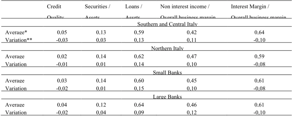
In the sample period, a process of re-arrangement of bank returns followed deep variations in the business model of banks. The non-interest income component raised above the traditional income sources, represented by net interest margin. This process substantially regarded the whole banking system, characterized by a similar production function, which highlights the multifunctional nature of single firms. However, some differences arise when observing the ratio between loans to customers and total assets, which represents the weight of the credit function with respect to the financial function in the banking system: over 12 years, the growth of this indicator was much higher for small banks than for bigger ones (see table 2).
Moreover, in various studies reflecting peculiar realities, interesting differences in the production technology among big and small banks typically emerge. The integration process of the banking system often appears adequate, while major uncertainties are still related to the consolidation process and to the lack of competitiveness. More relevant differences arise at geographic level. While the production function is quite similar for northern and southern situated banks, the overall business margin is much more affected by non-interest income for northern banks, while southern banks show a clear prevalence of the traditional business model. The credit quality trend turns out to be consistent with such dynamics. A bigger interest
margin weight accounts for the higher risk-premium of southern banks, which generally suffer from a higher riskiness, due to historical development delays, as reflected in more NPL and doubtful loans. We do not emphasize any differentiation on the basis of ownership structure, as, in general, we deal with multifunctional groups, which perform similar activities; furthermore, as governance is concerned, Italian laws allow some peculiarities for a number of subjects, which much relax the shareholders and market surveillance/control, as in case of Foundations being in corporate capital or in per capita voting case in the Cooperative Banks.
Therefore, the variables representing heterogeneity (multiplied for the northern banks dummy) are:
i) The interest margin to overall business margin ratio, ii) The total loans to total assets ratio.
These two parameters show the different environment in which Italian banks operate, and do not depend on the choices of the single production units. These parameters are therefore shift factors on the cost function.
The inclusion of heterogeneity factors improves the cost frontier specification and leads to a more significant measure of efficiency as derived from a random effects model. Each model comes from Pitt and Lee’s (1981), which is slightly different from the conventional random effects model in that the individual specific effects are assumed to follow a half-normal distribution.
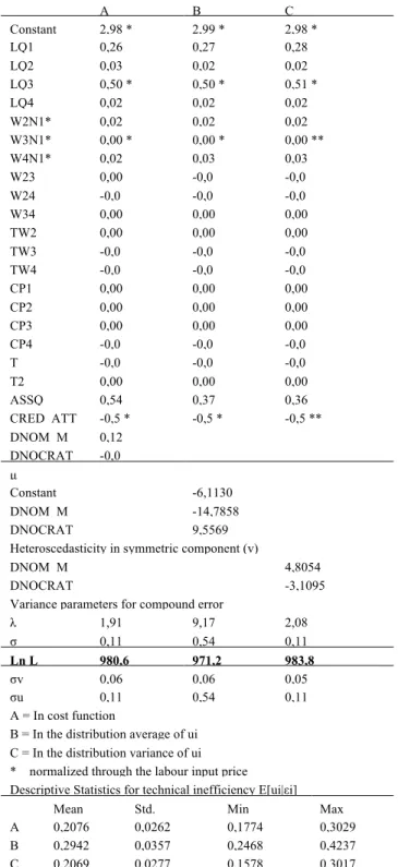
Parameters estimates are substantially stable under any specification. If heterogeneity is included in the cost frontier, the asset quality parameter increases very much, with respect to the panel estimate (0,55 against 0,43), highlighting a possible correlation with the exogenous components, whose significance is much limited. When exogenous components are included in the mean distribution of ui they show non-significant values. Both the σu estimate and the parameter λ rise significantly and,
therefore, the mean inefficiency value rises by about a third. Inefficiency estimates from model A and C display analogous mean values and standard deviations, while model B shows a much higher technical inefficiency. The most satisfactory specification is obtained when heterogeneity factors are inserted to explain the ui distribution variance (model C), despite the lack of strong theoretical justifications. Our choice of the favourite model is based upon likelihood reaching the maximum value , and on the inefficiency distribution, which appears slightly less concentrated (see table 3).
However, based on the correlation matrix, the efficiency and score values depend heavily on the heterogeneity assumptions (similar result can be found in Greene 2004b).
4. Time-variability of efficiency
An important hypothesis regarding efficiency estimate is the time-varying error term volatility. When time series span is long, the time invariance of inefficiency assumption
of both fixed and random effects models is likely to be problematic. However, inefficiency scores are more stable over time (and reliable) when inefficiency is small relative to industry-wide cost changes that occur at the same time, or when technology dispersion is imperfect. In order to cope with time variability of inefficiencies, the stochastic frontier model could be slightly modified into a ‘true’ fixed or random effects formulation as proposed by Greene (2005). While the former allows for freely time varying inefficiency, and allows the heterogeneity term to be correlated with the included variables, the latter includes a random (across firms) constant term.
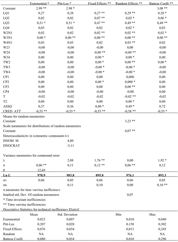
As shown in table 4, parameter estimates are consistent under various hypotheses (with the exception of credit quality), but efficiency values show high sensitivity to the time-varying volatility hypothesis. A scant relationship is displayed between time-invariant and time-varying inefficiencies: dispersion is quite remarkable. Time-invariant estimates are very different among productive units, with much higher mean value (0,207 in the case of Pitt and Lee heterogeneity adjusted model) as compared to time-varying estimates (0,076 for the fixed effects model). In this instance, the differences seem more likely to be due to the presence of cross bank heterogeneity, rather than to the assumption of time invariance of the inefficiency estimates. The gap between these descriptive statistics is confirmed by the wide underlying disagreement between the two sets of estimates; they are indeed substantially uncorrelated (the correlation coefficient is 0,1443 with respect to fixed effects and 0,0289 with respect to random effects). Therefore, we conclude that while estimates seem quite robust as regards the distributive hypotheses and to the choice of fixed or random effects, (as already observed in Greene 2004a, 2004b, 2005), the hypothesis of time variability of inefficiency affects to a large extent the estimated model, and especially the inefficiency levels. In general terms, both the efficiency measures and the scores show high sensitivity to the methodological choice and to output variables that represent the production process of the banks. However, once a robust specification is achieved, the efficiency estimate shows some persistency, keeping rather stable over time, as already noted by Kwan and Eisenbeis (1994), Berger and Humphrey (1991) and Berg (1992). A possible explanation is that time-invariant estimates are typically affected by heterogeneity not connected to inefficiency. In particular, if data shows some heteroskedasticity, it remains awkward to separate the effects on the stability of efficiency estimates over time, resulting from economies of scale rather than inefficiency.
If panel data are collected over a longer period of time, the problem of time series stationarity can assume a major role. At first sight, the variables included in the cost function are very likely to be non-stationary, but adopting a translog function can contribute to relax the problem.
In order to check our data we obtained (time-varying)
inefficiency estimates with the Battese-Coelli methodology (in that those estimates are highly correlated with the invariant Pitt and Lee case); statistical tests, although biased by the short number of observations, confirmed stationarity of inefficiency values. This result probably implies that technical progress, if any, is rather weak. In a phase characterized by growing integration of the banking system, gathering all benefits connected to M&A operations can really take time. In the Italian case this is all the more true when considering that the business dimension increase did not always give rise to new players and new activities, but more often it has involved overlapping functions among various players, as well as the survival of the old governance structures, so that the Acquisition operations prevailed over Mergers.
5. Concluding remarks
Structural changes of financial conditions and slackening in the potential output growth heavily affected the competitive environment of the Italian banking system. European integration pushed authorities to implement liberalization and deregulation rules of credit markets. As a result, there are now few banks with a larger size2.
Our scope is to disclose how much these phenomena have had impact on cost and productivity efficiency of banking institutions. Our contribution confirms the presence of a certain degree of inefficiency in the Italian banking system that, in the period 1993/2004, tends to persist over time, although showing some narrowing. The mean value of inefficiency is slightly higher than other studies suggest and close to 20%, mainly because of an improper use of scale factors and of input congestion. Deviations from the efficient frontier could moreover be brought about not only from managerial deficiency in choosing the input mix, but also from unsuitable comparison of non homogenous firms, that do not conform their behaviour to the “ideal” model. In order to analyze the role of heterogeneity and to discriminate between environmental factors and inefficiency strictly speaking, we compared the benchmark specification with alternative cost frontiers, based on specifications that include variables capturing heterogeneity. Such parameters operate therefore as shift factors on the cost function. The more satisfactory specification is obtained when heterogeneity is included in the variance of the distribution of the residual ui (capturing both technical
2 The banking crisis that was triggered in the spring of 2007 (the subprime crisis) had a little impact on the Italian banking system. In part this was due to the greater prudence that characterised the operational framework of the Italian commercial banks, based in particular on a deeper assessment of borrowers’ creditworthiness. Moreover, the local supervisory authority, the Bank of Italy, ensured a strict control of the systemic financial stability, so public bail-outs were extremely limited. Notwithstanding, some impact on capital structure, productive processes, and efficiency indicators arised. Such issues will be analysed in a future research.
and allocative inefficiency). Our result, although debatable on a pure theoretical basis, seems consistent in the light of likelihood reaching the maximum value and the lower concentration of inefficiency distribution. The inclusion of “environmental” factors affects the estimated values, leading to different mean efficiency and ranking values, both uncorrelated with the benchmark specification. The different specifications of heterogeneity turn out meaningful, especially for rankings rather than the efficiency measures. However, the units ranked in extreme position do not endure excessive modifications: in fact, the best and the worst 5 units are substantially the same ones under the various efficiency specifications. Further analysis could try to explain whether heterogeneity estimates are significant and why relevant inefficiencies do persist on the banking system over time. In presence of a complete and meaningful set of data, SFA could be able to find useful application in single event studies too, like those connected to rationalization and/or reorganization in banking firms.
Appendix
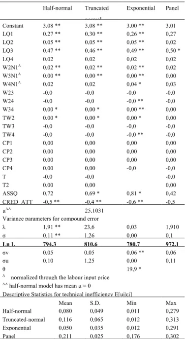
Table 1. Stochastic cost frontier under several error distribution assumptions
Half-normal Truncated normal Exponential Panel Constant 3,08 ** 3,08 ** 3,00 ** 3,01 ** LQ1 0,27 ** 0,30 ** 0,26 ** 0,27 LQ2 0,05 ** 0,05 ** 0,05 ** 0,02 LQ3 0,47 ** 0,46 ** 0,49 ** 0,50 * LQ4 0,02 0,02 0,02 0,02 W2N1A 0,02 ** 0,02 ** 0,02 ** 0,02 W3N1A 0,00 ** 0,00 ** 0,00 ** 0,00 ** W4N1A 0,02 0,02 0,04 * 0,03 W23 -0,0 -0,0 -0,0 -0,0 W24 -0,0 -0,0 -0,0 ** -0,0 W34 0,00 * 0,00 * 0,00 ** 0,00 TW2 0,00 * 0,00 * 0,00 * 0,00 TW3 -0,0 -0,0 -0,0 -0,0 TW4 -0,0 -0,0 -0,0 ** -0,0 CP1 0,00 0,00 0,00 0,00 CP2 0,00 0,00 0,00 0,00 CP3 0,00 0,00 0,00 0,00 CP4 0,00 0,00 -0,0 -0,0 T -0,0 -0,0 -0,0 T2 0,00 0,00 0,00 ASSQ 0,72 0,69 * 0,81 * 0,42 CRED_ATT -0,5 ** -0,4 ** -0,6 ** -0,5 ** µAA 25,1031
Variance parameters for compound error
λ 1,91 ** 23,6 0,03 1,910 0 σ 0,11 ** 1,26 0,00 0,1 Ln L 794,3 810,6 780,7 972,1 σv 0,05 0,05 0,06 ** 0,06 σu 0,10 1,25 0,00 0,11 θ 19,9 *
A normalized through the labour input price AA half-normal model has mean µ = 0
Descriptive Statistics for technical inefficiency E[ui|εi]
Mean S.D. Min Max Half-normal 0,080 0,049 0,011 0,279 3 Truncated-normal 0,116 0,065 0,012 0,313 7 Exponential 0,050 0,035 0,012 0,291 3 Panel 0,211 0,025 0,176 0,302 8
Table 2. Credit quality and banks business model (1993-2004) Credit Quality Securities / Assets Loans / Assets
Non interest income / Overall business margin
Interest Margin / Overall business margin Southern and Central Italy
Average* 0,05 0,13 0,59 0,42 0,64 Variation** -0,03 0,03 0,13 0,11 -0,10 Northern Italy Average 0,02 0,14 0,62 0,47 0,59 Variation -0,01 0,01 0,14 0,10 -0,08 Small Banks Average 0,03 0,14 0,60 0,45 0,61 Variation -0,02 0,01 0,15 0,10 -0,08 Large Banks Average 0,04 0,12 0,64 0,46 0,61 Variation -0,02 0,04 0,09 0,12 -0,10 * in percent
Table 3. Stochastic cost frontier under various heterogeneity hypotheses A B C Constant 2,98 * 2,99 * 2,98 * LQ1 0,26 0,27 0,28 LQ2 0,03 0,02 0,02 LQ3 0,50 * 0,50 * 0,51 * LQ4 0,02 0,02 0,02 W2N1* 0,02 0,02 0,02 W3N1* 0,00 * 0,00 * 0,00 ** W4N1* 0,02 0,03 0,03 W23 0,00 -0,0 -0,0 W24 -0,0 -0,0 -0,0 W34 0,00 0,00 0,00 TW2 0,00 0,00 0,00 TW3 -0,0 -0,0 -0,0 TW4 -0,0 -0,0 -0,0 CP1 0,00 0,00 0,00 CP2 0,00 0,00 0,00 CP3 0,00 0,00 0,00 CP4 -0,0 -0,0 -0,0 T -0,0 -0,0 -0,0 T2 0,00 0,00 0,00 ASSQ 0,54 0,37 0,36 CRED_ATT -0,5 * -0,5 * -0,5 ** DNOM_M 0,12 DNOCRAT -0,0 µ Constant -6,1130 DNOM_M -14,7858 DNOCRAT 9,5569 Heteroscedasticity in symmetric component (v)
DNOM_M 4,8054
DNOCRAT -3,1095
Variance parameters for compound error
λ 1,91 9,17 2,08 σ 0,11 0,54 0,11 Ln L 980,6 971,2 983,8 σv 0,06 0,06 0,05 σu 0,11 0,54 0,11 A = In cost function
B = In the distribution average of ui C = In the distribution variance of ui * normalized through the labour input price Descriptive Statistics for technical inefficiency E[ui|εi]
Mean Std. Deviation Min Max A 0,2076 0,0262 0,1774 0,3029 B 0,2942 0,0357 0,2468 0,4237 C 0,2069 0,0277 0,1578 0,3017
Table 4. Stochastic cost frontier - Time invariant vs. time varying inefficiencies
Exponential * Pitt-Lee * Fixed Effects ** Random Effects ** Battese Coelli **
Constant 2,99 ** 2,98 * 3,08 ** LQ1 0,27 0,28 0,27 ** 0,29 ** 0,28 * LQ2 0,02 0,02 0,07 ** 0,02 * 0,06 * LQ3 0,51 * 0,51 * 0,47 ** 0,49 ** 0,48 ** LQ4 0,03 0,02 0,02 0,02 * 0,03 W2N1 0,02 0,02 0,02 ** 0,02 ** 0,02 * W3N1 0,00 * 0,00 ** 0,00 ** 0,00 ** 0,00 ** W4N1 0,03 0,03 0,02 0,03 ** 0,02 W23 -0,00 -0,00 -0,00 0,00 -0,00 W24 -0,00 -0,00 -0,00 ** -0,00 ** -0,00 W34 0,00 0,00 0,00 * 0,00 * 0,00 TW2 0,00 0,00 0,00 * 0,00 ** 0,00 * TW3 -0,00 -0,00 -0,00 * -0,00 * -0,00 TW4 -0,00 -0,00 -0,00 * -0,00 * -0,00 CP1 0,00 0,00 0,00 0,000 0,00 CP2 0,00 0,00 0,00 * 0,000 * 0,00 CP3 0,00 0,00 0,00 0,00 ** 0,00 CP4 -0,00 -0,00 -0,00 -0,00 0,00 T -0,02 -0,02 -0,02 -0,02 ** -0,02 T2 0,00 0,00 0,00 0,00 * 0,00 ASSQ 0,37 0,36 0,80 * 0,49 * 0,72 CRED_ATT -0,55 ** -0,55 * -0,55 ** -0,58 ** -0,55 * Means for random parameters
Constant 3,23 **
Scale parameters for distributions of random parameters
Constant 0,07 **
Heteroscedasticity in symmetric component (v)
DNOM_M 4,80
DNOCRAT -3,11
Variance parameters for compound error
λ 2,08 1,76 ** 0,00 1,92 * σ 0,06 ** 0,11 0,12 ** 0,06 ** 0,12 θ 12,69 Ln L 970,9 983,8 895,8 976,1 893,3 σv 0,06 0,05 0,06 0,06 0,05 σu 0,11 0,10 0,00 0,10 **
η parameter for time varying inefficiency
Implied std. Dev. Of random parameters 0,07 * Time invariant inefficiencies
** Time varying inefficiencies
Descriptive Statistics for technical inefficiency E[ui|εi]
Mean Std. Deviation Min Max
Exponential 0,023 0,007 0,010 0,040 Pitt-Lee 0,207 0,028 0,158 0,302 Fixed Effects 0,076 0,034 0,013 0,245 Random Effects NA NA NA NA Battese Coelli 0,080 0,054 0,010 0,296
REFERENCES
[1] D. Aigner, C.A. Knox Lovell, P. Schmidt. Formulation and Estimation of Stochastic Frontier Production Function Models” Journal of Econometrics 6(1), 21-37, 1977. [2] Y. Altunbas, L. Evans, P. Molyneux. Bank ownership and
efficiency Journal of money credit & banking 33(4), 926-954, 2001.
[3] Y. Altunbas, J. Goddard, P. Molyneux. Technical change in banking Economic Letters 64, 215-221. 1999.
[4] B.H. Baltagi, J.M. Griffin. A general index of technical change Journal of Political Economy 96, 20–41, 1988. [5] Bank of Italy. Ordinary General Meeting of Shareholders,
Abridged Report for the year 2003, 2004.
[6] G.E. Battese, T.J. Coelli. A Model for Technical Inefficiency Effects in a Stochastic Frontier Production Function for Panel Data Empirical Economics 20(2), 325-332, 1995. [7] G.E. Battese, G.S. Corra. Estimation of a Production
Frontier Model: With Application to the Pastoral Zone of Eastern Australia Australian Journal of Agricultural Economics 21(3), 169-79, 1977
[8] S.A. Berg. Mergers, Efficiency and Productivity Growth in Banking: The Norwegian Experience 1984-1990 Working Paper, Norges Bank, Norway, 1992.
[9] A.N. Berger, R. DeYoung. Problem loans and cost efficiency in commercial banks Proceedings, Federal Reserve Bank of Chicago, May, 219-236, 1996.
[10] A.N. Berger, D.B. Humphrey. The Dominance of Inefficiencies over Scale and Product Mix Economies in Banking Journal of Monetary Economics 28, 117-48, 1991. [11] A.N. Berger, D.B. Humphrey. Efficiency of Financial
Institutions: International Survey and Directions for Future Research European Journal of Operational Research Special Issue on New Approaches in Evaluating the Performance of Financial Institutions, 1997.
[12] A.N Berger, Mester L. (1997) Inside the black box: what explains differences in the efficiencies of financial institutions? Journal of banking & finance 21(7).
[13] J.W.B. Bos, F. Heid, M. Koetter, J.W. Kolari, C.J.M Kool. Inefficient or just different? Effects of heterogeneity on bank efficiency scores Deutsche Bundesbank Discussion Paper Series 2: Banking and Financial Studies, n.15, 2005.
[14] J. Boyd, M. Gertler. Are Banks Dead? Or Are the Reports Greatly Exaggerated Federal Reserve Bank of Minneapolis Quarterly Review, Summer, reprinted in: The Declining Role of Banking?, Federal Reserve Bank of Chicago, 1994. [15] S. Carbò Valverde, D. Humphrey, R. Lopez del Paso.
Opening the black box: Finding the source of cost inefficiency Journal of Productivity Analysis 27(3), 209-220, 2007.
[16] B. Casu, C. Girardone. Does Competition Lead to Efficiency? The Case of EU Commercial Banks mimeo, XVI
International Tor Vergata Conference on Banking and Finance, 2007.
[17] A. Charnes, W.W. Cooper, E. Rhodes. Measuring the efficiency of decision making units European Journal of Operational Research 2(6), 429-444, 1978.
[18] J. Clark. Economic Cost, Scale Efficiency and Competitive Viability in Banking Journal of Money, Credit, and Banking 28, 342-64, 1996.
[19] J.A. Clark, T.F. Siems. X-Efficiency In Banking: Looking Beyond the Balance Sheet Journal of Money, Credit and Banking 34(4), 987-1013, 2002.
[20] P. Drummond, A.M. Maechler, S. Marcelino. Italy – Assessing Competitionn and Efficiency in the Banking System IMF Working Paper, 07/26, 2007.
[21] M- Filippini, J. Wild, M. Kuenzle. Scale and Cost Efficiency on the Swiss Electricity Distribution Industry: Evidence from a Frontier Cost Approach Working Paper n. 8, Centre for Energy Policy and Economics, Swiss Federal Institutes of Technology, Zuerich, 2001.
[22] D. Focarelli, F. Panetta, C. Salleo. Why do Banks Merge? Temi di Discussione Banca d’Italia, n.361, 1999.
[23] C. Girardone, P. Molyneux, E.P.M. Gardener. Analysing the determinants of bank efficiency: the case of Italian banks Applied Economics 36, 215-227, 2004.
[24] W. Greene. Frontier Production Functions In: H. Pesaran, P. Schmidt, (Ed.), Handbook of Applied Econometrics, Volume II, Microeconomics, Oxford University Press, Oxford, 1997.
[25] W. Greene. LIMDEP computer program: Version 8.0, Econometric Software, Plainview, New York, 2000. [26] W. Greene. The Separation of Technical and Allocative
Inefficiency In Antonio Alvarez, (Ed.) The Measurement of Firm Inefficiency, Cambridge University Press, 2003. [27] W. Greene. Fixed and Random Effects in Stochastic Frontier
Models Journal of Productivity Analysis 23, 7-32, 2004a. [28] W. Greene. Distinguishing Between Heterogeneity and
Inefficiency: Stochastic Frontier Analysis of the World Health Organization’s Panel Data on National Health Care Systems Health Economics 13, 959-980, 2004b.
[29] W. Greene. Reconsidering Heterogeneity in Panel Data Estimators of the Stochastic Frontier Model Journal of Econometrics 126, 269-303, 2005.
[30] W. Greene. The Econometric Approach to Efficiency Analysis, to appear as Chapter 2 in: Fried H., Knox Lovell, C.A., Schmidt S. (Ed.) The Measurement of Efficiency, Oxford University Press, 2008.
[31] S.C. Kumbhakar, C.A. Knox Lovell. Stochastic Frontier Analysis, Cambridge University Press, New York, 2000. [32] S.H. Kwan, R.A. Eisenbeis. An Analysis of Inefficiencies in
Banking: A Stochastic Cost Frontier Approach Working Paper, Federal Reserve Bank of San Francisco, U.S.A, 1994. [33] G. Lang, P. Welzel. Efficiency and Technical Progress in
Banking: Empirical Results for a Panel of German Cooperative Banks Journal of Banking and Finance 20(6),
1003-23, 1996.
[34] H.E. Leland, D.H. Pyle. Informational asymmetries, financial structure, and financial intermediation Journal of Finance 32, 371-387, 1977.
[35] W. Meeusen, J. van den Broeck. Efficiency Estimation from Cobb-Douglas Production Functions with Composed Error International Economic Review 18(2), 435-44, 1977. [36] H. Okuda, H. Hashimoto. Estimating Cost Functions of
Malaysian Commercial Banks: The Differential Effects of Size, Location, and Ownership Asian Economic Journal 18(3), 233-259, 2004.
[37] H. Okuda, F. Mieno. What happened Thai commercial banks in the pre-Asian crisis period? Hitotsubashi Journal of Economics 40(2), 97-121, 1999.
[38] M. Pitt, L. Lee. The Measurement and Sources of Technical Inefficiency in the Indonesian Weaving Industry Journal of Development Economics 9, 43-64, 1981.
[39] A. Resti. Regulation Can Foster Mergers, Can Mergers Foster Efficiency? The Italian Case Journal of Economics and Business 50, 157-169, 1988.
[40] P. Schmidt, R. Sickles. Production Frontiers and Panel Data Journal of Business and Economic Statistics 2(4), 367-374, 1984.
[41] H. Wang, P. Schmidt. One Step and Two Step Estimation of the Effects of Exogenous Variables on Technical Efficiency Levels Journal of Productivity Analysis 18, 129-144, 2002. [42] M. Weinstein. The Sum of Values from a Normal and a
Truncated Normal Distribution Technometrics 6, 104-105, 1964.