Fiber beam-columns models with flexure-shear interaction for nonlinear analysis of reinforced concrete structures

DOTTORATO DI RICERCA IN

INGEGNERIA STRUTTURALE ED IDRAULICA

Ciclo XXIII

Settore scientifico-disciplinare di afferenza: ICAR09

Fiber beam-columns models with flexure-shear interaction for nonlinear

analysis of reinforced concrete structures.

Presentata da: Filippo Cardinetti

Coordinatore Dottorato

Relatore

Chiar.mo Prof. Erasmo Viola

Chiar.mo Prof. Pier Paolo Diotallevi

Correlatore

Abstract

The aim of this study was to develop a model capable to capture the different contributions which characterize the nonlinear behaviour of reinforced concrete structures. In particular, especially for non slender structures, the contribution to the nonlinear deformation due to bending may be not sufficient to determine the structural response. Two different models characterized by a fibre beam-column element are here proposed. These models can reproduce the flexure-shear interaction in the nonlinear range, with the purpose to improve the analysis in shear-critical structures. The first element discussed is based on flexibility formulation which is associated with the Modified Compression Field Theory as material constitutive law. The other model described in this thesis is based on a three-field variational formulation which is associated with a 3D generalized plastic-damage model as constitutive relationship.

The first model proposed in this thesis was developed trying to combine a fibre beam-column element based on the flexibility formulation with the MCFT theory as constitutive relationship. The flexibility formulation, in fact, seems to be particularly effective for analysis in the nonlinear field. Just the coupling between the fibre element to model the structure and the shear panel to model the individual fibres allows to describe the nonlinear response associated to flexure and shear, and especially their interaction in the nonlinear field. The model was implemented in an original matlab® computer code, for describing the response of generic structures. The simulations carried out allowed to verify the field of working of the model. Comparisons with available experimental results related to reinforced concrete shears wall were performed in order to validate the model. These results are characterized by the peculiarity of distinguishing the different contributions due to flexure and shear separately. The presented simulations were carried out, in particular,

other computer programs. Finally it was applied for performing a numerical study on the influence of the nonlinear shear response for non slender reinforced concrete (RC) members.

Another approach to the problem has been studied during a period of research at the University of California Berkeley. The beam formulation follows the assumptions of the Timoshenko shear beam theory for the displacement field, and uses a three-field variational formulation in the derivation of the element response. A generalized plasticity model is implemented for structural steel and a 3D plastic-damage model is used for the simulation of concrete. The transverse normal stress is used to satisfy the transverse equilibrium equations of at each control section, this criterion is also used for the condensation of degrees of freedom from the 3D constitutive material to a beam element. In this thesis is presented the beam formulation and the constitutive relationships, different analysis and comparisons are still carrying out between the two model presented.

Table of contents

 

Chapter 1 - Inroduction

1.1  Sommario      1  1.2  Different approaches to the nonlinear analyses of reinforced concrete structures    1  1.2.1  Macroscopic approach      1  1.2.2  Microscopic approach      2  1.2.3  Global models      3  1.2.4  Fibre Models      10  1.3  Aim and objective of the thesis       13  1.4  Outline of the thesis      14 

Chapter 2 - Fibre beam-column element with flexure-shear interaction: state of

the art

2.1  Sommario      16  2.2  Fibre Beam‐Column Element Using Strut‐and‐Tie Models      17  2.2.1  Guedes’s Model      17  2.2.2  Martinelli’s Model      20  2.2.3  Ranzo and Petrangeli’s model      23  2.3  Fibre Beam‐Column Element Using Microplane Model      27 

2.4.2  Bentz’s Model      33 

2.4.3  Remino’ Model.      35 

2.4.4  Bairan’s Model      37 

2.5  Fibre Beam‐Column Element Using Damage Models.      41 

2.5.1  Modello di Mazars      41 

Chapter 3 - Fibre beam-column beam formulation

3.1  Sommario      44  3.2   Definition of the vectors involved      45  3.3  Formulation of the element starting from mixed method      46  3.4  Element state determination      48  3.4.1  Description of the procedure      49  3.4.2  Element state determination algorithm.      50 

Chapter 4 - Constitutive Relationship: Section state determination

4.1  Sommario      55  4.2  Modified compression field theory      56  4.2.1  Introduction      56  4.2.2  Compatibility condition       56  4.2.3  Equilibrium Condition      57  4.2.4  Constitutive relationship      59 

4.3.2  Equilibrium equation      65 

4.3.3  Compatibility relations      67 

4.3.4  Constitutive Relations      69 

4.3.5  Shear slip  model      71 

Chapter 5 - Implementation of the model

5.1  Sommario      74  5.2  Definition input vectors and matrices      75  5.3  Algorithm steps       77  5.3.1  Structure state determination      80  5.3.2  Element state determination      81  5.3.3  Section state determination      83  5.4  Solution strategies      89  5.5  Flow Chart      91  5.5.1  Structure state determination      91  5.5.2  Element state determination      92  5.5.3  Section state determination       93 

Chapter6 - Numerical analysis and validation

  6.1  Sommario      97 

6.2  Comparisons between numerical and experimental results      98 

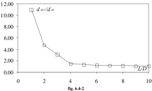
6.4  Investigation on the influence of flexure‐shear interaction      107  6.4.1  Parametric analysis on bridge pier      107  6.4.2  Parametric analysis on a shear wall      111  6.4.3  Analysis with the ratio   (slender shear wall) L/D=10.      111  6.4.4  Analysis with the ratio L/D=2 .      116  6.4.5  Analysis with the ratio  L/D=1.      118 

Chapter 7 - Alternative formulation for the shear critical beam-column element

(developed in University of California Berkeley)

7.1  Sommario      121  7.2  Finite element formulation      122  7.2.1  Kinematic assumptions       122  7.2.2  Hu‐Washizu Functional       122  7.2.3  Force interpolation matrix      126  7.2.4  Descripion of the shear forces      126  7.2.5  Section deformation and stiffness matrix      127  7.3  Constitutive relationships.      128  7.3.1  Steel material model      128  7.3.2  Concrete material model      130 

Conclusion

       134 

References

      137 

C

HAPTER

1

Introduction

1.1 Sommario

In questo capitolo introduttivo verranno trattati i criteri di modellazione della risposta sismica non lineare di strutture in c.a. Si riporta sia una classificazione delle diverse tipologie di modelli, sia una descrizione degli aspetti che sono stati sviluppati e perfezionati nel corso degli ultimi decenni. Vengono poi richiamati alcuni modelli e, senza entrare nel dettaglio, se non evidenziando le caratteristiche salienti. In questo modo è possibile inquadrare meglio le proprietà e le assunzioni su cui si basano i modelli proposti.

1.2 Different approaches to nonlinear analysis of reinforced concrete

structures

The study of reinforced concrete structures under strong seismic actions requires the formulation of analytical models capable of describing the behaviour of structural elements subject to cyclic loading in the non-linear fields, taking into account the typical phenomena of progressive deterioration of stiffness and strength. the following approaches can be distinguished in relation to the complexity and the model scale.

1.2.1 Macroscopic approach

Structural modeling of the is made trying to achieve a correspondence between the structural members and the elements of the analytical model. To this end, the one-dimensional elements are used to simulate the response of a beam, columns, or a wall portion between two floors. Following a macroscopic approach the effects of geometry details can be lost, such as the exact form of longitudinal and transverse reinforcement, but the main aspects of structural behavior can be reproduced quickly and the spread inelastic deformations along the element can be considered.

A typical example of the macroscopic approach are the global models. The constitutive laws for this kind of modes, are introduced in terms of section forces-section deformation such as moment-curvature relations. These approximation are sufficiently accurate to

hysteretic model. The reduced computational time and accurate simulation of the global hysteretic behavior, makes these models the most efficient method for the analysis of complex structures, consisting in a large number of elements.

The class of fiber models can be set in a macroscopic approach, indeed each structural element can be described by a single finite element, and the equilibrium and compatibility conditions are expressed in global terms. The sections behavior is studied through a discretization into finite areas, or, for planar elements, in strips. The constitutive relationships are locally defined, in terms of stress-strain relation for each fiber. Therefore, the fiber models are considered as intermediate between local and global formulation. At one side fiber model are based on simplified kinematic assumptions that allow to reduce the number of equations, to the other hand the global behaviour is derived from the materials constitutive laws. However fiber models requires remarkable computational effort, especially in complex structures analysis.

1.2.2 Microscopic approach

The structure is discretized with a large number of two or three-dimensional finite elements, using different elements for concrete, reinforcement and the bonds between the two materials. It’s much more accurate in describing the local behavior, but requires an excessive computational time. The use of microscopic models allows, at the most, to run analysis of individual elements or portions of structures, such as walls, beam-column or nodes.

1.2.3 Global models

The modeling of seismic behavior of reinforced concrete structures in the last forty years' was the focus of many researchers and led to the development of multiple types of global models. Since the late 60s were proposed simple models, which over the years have been improved and expanded.

This introduction it is focused on the elements for non linear analysis of structures, in which the shear strength is enough to ensure the development of inelastic deformation. In this context, global models can be classified in relation to the inelastic deformation distribution, with this criteria may have lumped plasticity elements and distributed plasticity elements.

The nonlinear behavior of frame structures of usually concentrated in critical areas corresponding to the beams-columns ends. So one of the first approaches to modeling this behavior has been carried out assuming a zero-length plastic hinges as a rotational springs located at the ends of the beam-column elements, and connected in series or in parallel, depending on the type of connection may have series or parallel models as shown in fig. 1.2-2

The first component model was introduced in parallel by Clough et al. (1965), and is shown in fig. 1.2-3. The model consists of two elements in parallel, one elastic-perfectly plastic, to represent the yield strength, and the other elastic with a reduced stiffness to reproduce the hardening. The element stiffness matrix is the sum of those of the two parallel elements. The advantage of these models, also called "two component model", lies in the independence of the formulation from the moments diagram, while the problem arise from the fact that this kind of elements allow to use only a bilinear moment-curvature relation, so it is incapable of represent the typical degradation of reinforced concrete elements. These models, overestimate the energy dissipation capacity of reinforced concrete structural elements.

fig. 1.2-2

Clough et al. (1965) Giberson (1967).

Series models were introduced to overcoming the limitations inherent in the parallel models. They were formally introduced by Giberson (1967), the model (fig. 1.2-3) consists of two non-linear rotational springs and end of an elastic beam. For each spring is introduced a moment-rotation relationship assuming an antisymmetric linear distribution of moments along the element. In series models the flexibility matrix of each spring is summed with the flexibility matrix of the linear elastic beam. This type of models are much more versatile than the parallels, with series models is possible to describe a more complex hysteretic behavior, selecting an appropriate moment-rotation relationship for springs, but they are limited by the assumption of a constant moments distribution along the element. Suko and Adams (1971), proposed to take the contraflexure point from the initial elastic analysis instead of the center of the beam. Otani (1974), proposed a more sophisticated model, shown in fig. 1.2-4. The Otani’s model consists of two deformable parallel elements, one linear elastic and the other non-linear, two rotational springs and two rigid connection at the ends to take into account the finite size of the beam-column node. The rotational springs are used to consider the effects of the reinforcement slip at the nodes. The construction of the flexibility matrix is based on the calculation of the contraflexure point step by step. The element is treated as two cantiliver beams, with a free end at the contraflexure point. With this assumption the element is equivalent to two inelastic rotational springs at the ends, whose properties are related to the current position of the contraflexure point. The Otani’s model, however, is not capable to evaluate the actual spread inelasticity along the element, depending not only on the current state of the element, but also on the load history.

Concentrated plasticity models have been formulated neglecting the phenomena of axial force-moment interaction. The moment-rotation relationship are defined referring to a constant value of axial force, usually the gravity loads. Actually, the normal stress in the columns due to seismic action can vary significantly, affecting both the resistance and the stiffness properties of structural elements. Considerable efforts have been made to include the effects induced by the variations of normal stress in simplified models, but this kind of models are not applied extensively. Saatcioglu et al. (1983) introduced a concentrated plasticity model, in which the moment-rotation relationship of the springs is characterized by a family of curves, each corresponding to a different value of normal stress.

An important step in the modeling of axial force-bending moment interaction, was made with the introduction of multispring models, which are classified between as concentrated plasticity, but actually these differ considerably from those described above, and in somehow are similar to simplified fibers models. The first multispring model was proposed by Lai et al. (1984), it was constituted by a central elastic element, and a series of axial springs at the end zones to simulate the inelastic response (fig. 1.2-5). The non-linear deformations are concentrated in the end zone, although their behavior is not defined by

the moment-rotation relation, but through a discretization of such zones in areas that represent the springs.

In the Lai’s model each inelastic element consists of five spring for concrete, four for corners and a central one, and four for steel. The force-displacement relationship for the steel springs follows an hysteretic model with degradation similar to that assumed on the moment-rotation relationship viewed for others concentrated plasticity models. The elongation of each spring is correlated with the average axial displacement and the section rotation, through the assumption of plane sections remain plain.

Saiid et al. (1989), proposed a multispring model with five springs based on Lai et al. (1984). One spring is central to simulate concrete core, while four springs are placed at sides to simulate the behavior of a reinforced concrete element subjected to axial elongation, corresponding to the area represented by each spring. With this model the authors overcame some inherent inconsistencies in the Lai’s model, and have performed good comparison with experimental tests.

The best feature of multispring models is the ability to simulate with good accuracy the nonlinear behavior of spatial columns, requiring much lower computational effort than fiber models.

The concentrated plasticity models, as seen above, are not able to take into account the gradual spread of inelastic deformation within the elements. A more accurate description of the nonlinear behavior of reinforced concrete elements is possible by using distributed plasticity models. These kind of models assumes that the inelastic deformation may occur in any section, the element response is derived through an integration of sections response along the element.

Schnobrich and Takayanagi (1979), have proposed to divide the element into a finite number of segments (fig. 1.2-6), each with constant properties dependent on the bending moment at the midpoint. Each segment is studied through a moment-curvature relation including the effects of degradation due to cyclic loading. Also in this model a proposal to take account the axial-bending interaction is made. The section stiffness is defined, including axial effects, as resulting from predefined interaction diagrams.

Analyze the sections response along the element leads to various difficulties, for the greatest calculation time and for the numerical problems related to the arise of unbalanced moments within the element. Equilibrate these moments requires the introduction of complex procedures not necessary when are studied only the end sections. Therefore, several authors have developed concentrated plasticity models able to take into account the gradual spread inelasticity. These models, also called distributed inelasticity have been widely used, and many computer codes have been based on them.

In fig. 1.2-6 is shown the Meyer’s model, Meyer et al. (1983) and the later one improved by Roufaiel and Meyer (1987). The element is divided into three zones, one central elastic and two inelastic ends, varying in length depending on the load history.

This formulation is independent from the position of contraflexure point, and take into account the coupling of the inelastic deformation in the two non linear segments. The properties of these segment are derived by simplified assumptions on the end sections, carried out through hysteretic moment-curvature models

Schnobrich and Keshavarzian (1985), have adopted the same element, but taking into account axial-flexure interaction. To consider these effects they followed a similar approach to that proposed by Takayanagi and Schnobrich (1979).

The criteria used by Meyer et al. (1983) is part of the formulation of Filippou and Issa (1988), and Mulas and Filippou (1990), which added to the element, two rotational springs at the extremities, for take into account the fixed end rotation at the beam-column joint, due to bar pull-out.effects. These authors have attempted to define more accurately the moment-rotation relationship of the springs, which was independent from the assumed moment-curvature relationship at the end sections. Filippou Ambrisi (1997) have included more non-linear springs to account for translational non-linear deformations due to shear. This model is made up of several sub-elements connected in series to distinguish the various aspects that affect the nonlinear behavior of the structural element.

A further evolution was carried out by Aredia and Pinto (1998) dividing the element into three zones. They have developed a method to identify, in the elastic part of the element, cracked and uncracked zones. Their model is based on the assumption that the elastic limit

Schnobrich and Takayanagi (1979) Roufaiel e Meyer (1987).

may be exceeded only in the end zone, and that the cracked areas can be developed at both of them, both from the central section of the element, where it is possible to apply a concentrated load. Both areas, cracked and plasticized have variable length depending on the loading history, determined by taking a linear progression of bending moment from each end to the center of the beam.

A common plasticity model that differs from those just described was carried out by Kunnath et al. (1990), this model can perform local and global damage evaluation as well as non-linear seismic analysis of reinforced concrete structures. Kunnath et al. (1990) did not directly assess the length of the plasticized hinges. The element characteristics will be deducted from the sections by integration, assuming a flexibility distribution piecewise linear (fig. 1.2-7) .

This distribution is identified by the beam ends flexibility, that come from the moment-curvature relationship, and from the flexibility of the contraflexure point, which is assumed to be equal to the elastic value.

1.2.4 Fibre Models

In Fibres models is carried out a double discretization, in the longitudinal direction difining a predetermined number of sections and in the transverse direction, discretizing in small finite areas the element cross sections. In case of simple planar bending model is sufficient to subdivide the sections into strips perpendicular to the axis of flexion, in the more general spatial cases a double subdivision into small rectangular areas is required

(fig. 1.2-8). Each fiber, represent a corresponding portion of elementary concrete or reinforcement area , by integration over the cross section is possible to obtain moment-curvature relationship, and thus determines the overall response of the whole element. By the hypothesis of plane sections remain plane, axial deformation of each fiber ε( , )x y can be obtained, once knowing curvature χx, χy and axial deformation ε0 referred in section

centroid.

0

( , )x y y _z z _x

ε =ε + ⋅χ − ⋅χ (1.3.1)

The characteristics described above are common to all models, so that not changes in different element formulations. What really change in different fibre models is essentially the state determination procedures that depend on different formulation. In fact fiber models, as distributed plasticity models, has the problem, highlighted in previous paragraph, about the arise of unbalanced section forces within the element. After a load step application, nodal displacement are calculated and from these the section forces can be evaluated, but because of the materials nonlinear behavior in all control sections, resisting forces doesn’t match section forces.

In global models, especially those with concentrated plasticity this problem is not treated because only the end sections are taken into account. Fibre models differ therefore in the process used to determine the section resisting forces. Different procedure has been proposed depending on the element formulation, in particular can be found procedure for stiffness based, flexibility based or mixed elements.

The early models have been developed on a stiffness based approach, using classical shape functions. A model that use this approach is due to Aktan et al. (1974), in which nodal resisting forces are obtained directly from section resisting forces by applying the virtual work principle. The formulation is compatible, however, it is shown that is inadequate in nonlinear cases because it involves a linear curvature distribution over the length. This assumption is unrealistic for reinforced concrete elements in nonlinear field.

The latter models become increasingly based on a flexibility approach, this class of models uses forces interpolation functions, thus a balanced element is achieved while in stiffness models the compatibility was the basic assumption. One of the first balanced element is proposed by Kaba and Mahin (1984), based on Aktan (1974), this model introduce the displacements interpolation functions updated for each load increment through the flexibility matrix. In this model, however, the numerical problems discussed above have not been solved because the theoretical formulation is not totally consistent with the flexibility approach.

Essentially the flexibility approach is more realistic than the stiffness based one, but involves significant problems in determining the nodal resisting forces. Many studies, therefore, have attempted over the years to overcome these problems. Zeris and Mahin (1988, 1991), developed a complex iterative procedure to investigate the cross section deformation associated with internal balanced forces, with a shape coincident with forces interpolation functions. Taucer et al. (1991) have proposed a model that is part of a more general mixed approach. The nodal resisting forces are calculated for each element through an iterative procedure. At each iteration, are calculated the residual nodal displacements associated with the unbalance section forces along the element. The main characteristic of this model is that, at each iteration, compatibility and equilibrium are satisfied within the element. Taucer et al. (1991) show that the proposed algorithm is effective even if the

Finally some recent developments in fiber models are oriented in the attempts to develop extensions in classical elements including other sources of nonlinear deformation, such as those related to shear stress. In this class of models, widely described in chapter two, the section state deformation is characterized not only by the axial deformation and the curvature in the centroid, but also by the shear deformation evaluated in nonlinear field. Besides the hypothesis of plane sections remain plane, a given distribution of shear deformation is assigned in order to detect the state of deformation of each fiber. Generally a biaxial stress-strain relationships is associated to these elements. This model is very close to a microscopic approach, but compared to the that has the same degrees of freedom of beam element type.

In conclusion, fibre models requires a large number of operations to evaluate the element stiffness matrix, the stress and strain state in each section. In other words fibre models are really time consuming in state determination procedures. Although sometimes it incurs in numerical stability problems, many advantages can be identified using these models as:

ƒ Catch the actual evolution of plasticization along the element ƒ Are able to reproduce realistically pinching phenomena

ƒ Describe in detail geometry and position of transverse reinforcement ƒ Can reproduce the interaction between axial forces and bending moments ƒ Can be easily implemented spatial elements.

Also the constitutive relationship are more easy to implement because the singles materials are considered instead of moment-curvature relationship.

In this thesis a fibre model able to take into account the coupling between moment, axial forces, and shear in non-linear field is presented. It is based on the flexibility approach to take advantage of the benefits attributed to this class of fiber model, in particular between all fibre modes has been chosen Taucher et all. (1991) because it seemed to respond better to requests features.

1.3 Aim and objectives of the thesis

The main purpose of the thesis is to propose a finite element able to model structures, where the shear deformation appears predominant. The category of models chosen to attain this goal are the fiber models, treated in the previous chapter. As highlighted in the

overview in this introduction, the shear deformation and in particular the shear-flexure coupling in nonlinear field is still an open research topic, in particular, in global models as beam-column elements.

This aim will be achieved through the following enabling objective:

ƒ To gather information on existing knowledge about flexure- shear interaction in fibres models, through a comprehensive literature review.

ƒ To develop and implement an efficient fibre model, capable of predicting the behaviour of concrete squat structures, which include a bidimensional theory for concrete (Modified Compression Field Theory) as constitutive relationship.

ƒ To validate the model by comparing the predicted behaviour with the behaviour observed in experimental results, in particular the model must reproduce the global response of the structure with reasonable agreement with experimental evidence. ƒ To validate the model by comparing the results with another code with different

approach and carrying out a parametric analysis with the aim of study the influence of flexure-shear interaction by varying the slenderness.

ƒ To illustrate a different model proposed, based on a different formulation and a different constitutive relationship , with the aim of proposing an alternative model with which, will carry out future comparison and mutual improvement.

1.4 Outline of the thesis

The contents of the thesis will be divided into different chapters as follows:

ƒ The first chapter is introductory, recalls some basic concepts of nonlinear analysis and models categories. In this chapter can be found descriptions of concentrated plasticity elements (one component and two components model) , distributed plasticity elements and fibres models, focusing on the stiffness and flexibility formulations highlighting the benefits and the deficiency of each approach.

ƒ The second chapter is entirely dedicated to the state of the art of fibres beam-column element, in which some author tried to introduce shear deformation. In this chapter will be discussed in detail each of these models, from the strut and ties, to Microplane and smeared crack to finish with damage models.

ƒ In the third chapter will be treated the finite element formulation, will be described in detail the derivation of the flexibility based element, starting from the two-fields mixed method. This chapter describes how numerical procedures for structural and element determination have been carried out.

ƒ The fourth chapter is entirely dedicated to section state determination, through the description of MCFT (modified compression field theory) and DSFM (distrurbed stress field model) that are the basis of the constitutive law implemented in the model. For each theory will be analyzed compatibility, equilibrium and constitutive relationships for the average quantities between the material cracks, will be explained the equilibrium problem on cracks location and shear slip over the cracks.

ƒ In the fifth chapter will be explained the implementation of the model, this chapter will show the vectors and matrices involved in the program and the flow charts of the code. Furthermore will be explained in detail how the theories on which the model have been based are unified in a single computer code.

ƒ The sixth chapter will report all tests and comparisons performed with the computer code. First of all will be presented the reproduction of the experimental test conducted by Osterele et al. (1979). Then will be shown the numerical comparison between the computer program Vector2, developed at University of Toronto, and the code proposed in this thesis. Finally, two parametric analysis conducted on a bridge pier and on a shear wall, show how the nonlinear flexure-shear interaction actually affect the response in squat structure. Different analysis are carried out with the aim of evaluate this influence varying the structural slenderness.

ƒ The seventh chapter describe the formulation the constitutive relation and the implementation of the model studied at University of California Berkeley. This model represent an alternative solution to the presented problem, some comparison between the two models are in progress. For the element formulation has been used a three-field variational formulation while for constitutive relationship a three-dimensional material model. For concrete has been implemented a damage model with two parameters, one for tension and one for compression Lee and Fenves (1998), while for steel structures has been implemented a classical plasticity model.

C

HAPTER

2

Fibre beam-column element with flexure-shear interaction:

state of the art

2.1 Sommario

Tra i vari approcci adottati per eseguire delle analisi non lineari di strutture in c.a. gli elementi a fibre hanno mostrato una grande capacità di riprodurre l’interazione tra sforzo assiale e momento flettente, mentre l’accoppiamento di sforzi normali, flessionali e taglianti è un fenomeno ancora poco chiaro.

La soluzione al problema della modellazione taglio-flessione è stata affrontata in molti studi con approcci diversi. Un aspetto che caratterizza molti dei modelli proposti è il disaccoppiamento di flessione e taglio. Ad esempio, nei modelli “strut and tie” il classico elemento trave è associato ad un traliccio che simula il meccanismo resistente a taglio. In alcuni casi i modelli “strut and tie” sono stati combinati con elementi a fibre, come nei modelli proposti dalla Guedes e Pinto (1997), Martinelli (2002) e da Ranzo e Petrangeli (1998). Un altro metodo seguito per predire la risposta taglio-flessione si basa sulla teoria Microplane studiato da Bazant e Oh (1998), Bazant e Prat (1998) e da Bazant e Ozbolt (1990). L'approccio Microplane permette la descrizione della risposta multiassiale attraverso la combinazione di relazioni costitutive monoassiali. Petrangeli et al. (1999) usarono la teoria Microplane all'interno di un elemento a fibre.

Un altro approccio si basa sui modelli a fessurazione diffusa Vecchio e Collins (1988). In questo approccio, il calcestruzzo fessurato è modellato come un materiale ortotropo, in cui equilibrio e di compatibilità sono formulati in termini medi di tensione e deformazione.. Remino (2004) ha sviluppato un elemento a fibre con un legame costitutivo basato su Rose (2001). Ceresa et al. (2008) hanno realizzato un modello a fibre basato su una formulazione in rigidezze considerando la modified compression field theory (Vecchio e Collins (1996)) come legame costitutivo. Una particolare tipologia di modelli, come quella presentata da Mazars et al. (2006), implementano anche la teoria del danno.

2.2 Fibre Beam-Column Element Using Strut-and-Tie Models

This approach considers a Timoshenko fibre beam-column element, which is coupled with a truss structure. All the shear action is carried by the truss members. There are several models that adopt this technique, these models are presented below.

2.2.1 Guedes’s Model

Guedes et. al. (1994-1997) proposed a two-node 3D beam-column element based on a displacement formulation, with linear shape functions for axial displacement and rotation. The degrees of freedom per node are six, three displacements and three rotations::

( )x = ⎣⎡u x( ) v x( ) w x( ) θx( )x θy( )x θz( )x ⎤⎦

u (2.2.1)

On section, the axial components are obtained through a classical fibre model, while the shear components are obtained independently by a truss model (fig. 2.2-1).

fig. 2.2-1

The truss consists in two concrete struts whose slope represents the direction of principal stresses and strains, and longitudinal and transverse steel beam. The equilibrium and compatibility are shown in fig. 2.2-2

fig. 2.2-2

Referring to fig. 2.2-1 and fig. 2.2-2, the equilibrium between internal and external forces must be satisfied according to the equations:

1 2 ( ) sin 0 wy c c F + F +F ⋅ θ = (2.2.2) 1 2 ( c c ) sin 0 V + F −F ⋅ θ = (2.2.3)

The iterative procedure begins by estimating the value of ε_wy, the principal strains are calculated using the following:

( )

2

( )

2 ₂

(

)

0

tan

cos sin sin(2 ) 2,1

/ cos 2 i i e wy i l γ ε ε φ ε φ φ θ Δ = = ⋅ + ⋅ ± ⋅ = (2.2.4)

Where ε₀e=l₀e/l e γ are the kinematic parameters derived from Timoshenko beam theory and ε_wy = Δ_wy/h is the deformation in the stirrups calculated iteratively by the

equilibrium in the cross section. The forces in the principal direction can be calculated as follow:

(

)

( )

(

)

( ) ( ) 1 cos 1, 2

ci c i strut c i i w

F = f ε ⋅A =σ ε ⋅ −D ⋅ ⋅b h⋅ φ i= (2.2.5) Where D is a damage parameter, _i b_w⋅ is . Knowing h F F_{c1 c2} eφ the force F can be _wy

calculated from (2.2.2) and used to find ε_wy from the following equation:

( ) (

)

( ) 2 tan wy sw wy sw h F f A s ε φ = ⋅ ⋅ ⋅ ⋅ (2.2.6)

If the two subsequent values ofε_wy match with a predetermined tolerance, the solution is found, otherwise the iterative procedure continue. At the end of each iteration shear resisting forces V are estimated for each cross section.

The stiffness matrix, which the authors suggest to use, is derived from classic Timoshenko beam element keeping uncoupled flexure and shear. the following consideration can be made:

• The nonlinear behavior is derived from the use of the uniaxial constitutive relationship σ ε− , the tangent modulus is obtained step-by-step. The costitutive relationship used by the author is shown in fig. 2.2-3

• A simple liner elastic relationship can be used to represent the relation between the shear forces V and the shear deformation γ in the truss model.

fig. 2.2-3

This was one of the first attempts to model the shear behavior in a fiber element. The model presented is a 3D beam-column element, but the shear is modeled with a 2D mechanism. Furthermore, the truss model is not able to take into account other shear resistance mechanisms such as dowel action, arch action, aggregate interlock, compressive concrete that contribute to increase the beam-column shear capacity.

Questo fu uno dei primi tentativi nel quale si cercò di modellare il comportamento a taglio in un elemento a fibre.

Another limitation is represented by the inclination of the cracks that is fixed, equal to 30 ° or 45 °, further the truss model is not able to catch the coupling between axial flexure and

shear, in other words, the shear force has no effect on flexural response. The numerical verification highlight that the model did not represent the crack-closing phenomenon, so the pinching effect is amplified.

2.2.2 Martinelli’s Model

Martinelli (1998-2002) developed a model fibre beam-column element with the aim of evaluating the cyclic response of squat bridge piers. The author proposed a finite element superimposing a classical fibre model for the flexural deformations to a truss for shear deformations. The model is a classic 3D fibre element, based on a Timoshenko beam theory, formulated using a displacement-based approach. The element is a three-node beam with the intermediate node with only two degrees of freedom, rotations and axial displacement. The shear-locking phenomenon is avoided by keeping a mean constant shear deformation along the element and a linear curvature variation Crisfield (1986).

The displacement vector ( )u x is represented as follow (fig. 2.2-4).

( )u x = ⎣⎡u x( ) v x( ) w x( ) θy( )x θz( )x ⎤⎦T (2.2.7)

fig. 2.2-4

The shear resultant over the cross-section is the results of many different resisting mechanisms as the arch action, the truss mechanism, the compression concrete above the neutral axis, and the aggregate interlock, each of which considered independently.

The arc mechanism is shown in fig. 2.2-5 (a) where it’s observed that an inclined strut transfers a shear force proportional to the axial force V = ⋅N tan( )α .

fig. 2.2-5

The fibres are aligned with the strut, the inclination α, is calculated from the nodal moments

(

Mzi,Myi,Mzf,Myf

)

, and the centre of compressive stresses. Known α e εxx,

assumingε_yy = , the principal direction 0 ε₂ and the shear deformation 2

γ

can be calculated by the Mohr circle fig. 2.2-5 (b). An uniaxial constitutive relationship is used to deduce σ₂ from ε₂ (with the assumption of zero tensile principal stress σ₁= ). Known 0 σ₂ and γ

xx

σ and τ_xy are derived from Mohr's circles. The tensions thus obtained are integrated on the cross section to get the resisting forces.

cc xx y xx z xx A A A pxy xx pxy xz A A N dA M z dA M y dA V dA V dA σ σ σ τ τ = = ⋅ = ⋅ = =

∫

∫

∫

∫

∫

(2.2.8)

An Iterative procedure is required to calculate α. the authors suggest to take α as the value at the end of the previous step in a step-by-step dynamic analysis.

The truss mechanism is based on a 2D structure composed by the transverse reinforcement and the concrete diagonals in tension and compression as shown in fig. 2.2-5 (c). The diagonals are inclined by an angle φ assumed equal to the cracks inclination. The deformation of the truss is obtained from the kinematic parameters of the Timoshenko

beam ε_xx and γ_xy whereε_yyit is assumed equal to the strain in the stirrups and is calculated by imposing the equilibrium of the truss along y σ_yy = . 0

Using the Mohr circles of the principal directions are simply calculated, and τ_xy can be deduced by knowing the principal stresses. The shear transferred by the truss is calculated by integrating the shear stress over the tensioned concrete in the cross section V_t =τ_xy⋅ . A_t

concrete tangent modulus E and ₁ E in principal direction and steel tangent modulus ₂ s

E can be also evaluated. By the tangent modulus is possible to calculate the stiffness

matrix Kshear associated with the contribution of the truss.

The interlocking mechanism, is taken into account assuming a set of diagonal cracks with constant spacing s (s a model parameter), inclined by an angle φ kept constant, respect to the beam axis. The shear component τxyIN on the cross section are derived from the stresses

arising at crack faces, due to the relative displacement. These stresses are calculated from the strains ε_xx, γ_xy e ε_yy = derived from the truss mechanism. The shear force ε_s associated to the interlocking mechanism is derived from the integration of the shear stresses τ_xyIN over the tensioned concrete area: V_IN =τ_xyIN ⋅ A_t

The shear resistance force is given by the sum of the contribution of V , _p V e _t V and the _IN

stiffness matrix of the section is the following:

2 2 0 0 0 0 0 0 0 0 0 0 0 0 0 0 A A A A A A s A A A shear shear

EdA y EdA z EdA

y EdA y EdA y z EdA

z EdA y z EdA z EdA

⎡ _{− ⋅ ⋅} ⎤ ⎢ ⎥ ⎢ ⎥ − ⋅ ⋅ − ⋅ ⋅ ⎢ ⎥ ⎢ ⎥ = ⎢ _{⋅ − ⋅ ⋅ − ⋅} ⎥ ⎢ ⎥ ⎢ ⎥ ⎢ ⎥ ⎢ ⎥ ⎣ ⎦

∫

∫

∫

∫

∫

∫

∫

∫

∫

K K K (2.2.9)

where E is the elastic tangent modulus and K_shear is obtained by the truss mechanism.

A positive characteristic of this model is that it takes into account different shear resisting mechanisms. In particular, the arch effect and the flexural behavior are formulated in 3D, while other mechanisms are studied separately in planes xy and xz.

This means that the actual spatial behavior of the model is sometimes lost. It is also noted that in the arch effect the contribution of the shear depends on α and ε_xx, that are flexure-dependent parameter, so flexure and shear in the truss mechanism are actually coupled. In the truss mechanism the inclination of the cracks and the crack spacing are assumed constant, thus the effect of the longitudinal reinforcement is no taken into acount.

The deformation involved are γ_xy and ε_yy(neglected in the arch mechanism) are calculated iteratively until the equilibrium in y direction is reached.

The solution of the aggregate interlock is derived from the truss mechanism, in terms of strains, thus the aggregate interlock is not able to influence the other mechanisms, in particular, is not able to affect the principal stresses directions.

In the sectional stiffness matrix the shear contribution is given only by the truss mechanism and it is uncoupled from the flexural term. It could imply low convergence rate.

The comparisons with experimental results highlight some lacks of the model: first of all the capability to capture some specimen collapse, furthermore it tends to exaggerate strength degradation in cycles.

The model proposed by Martinelli [1998, 2002] is able to take into account different shear resistance mechanisms studied independently. While failing to capture a full coupling between axial, flexure and shear forces, it still can capture the behaviour of reinforced concrete with shear-influenced response with a very reasonable accuracy.

2.2.3 Ranzo and Petrangeli’s model

Ranzo and Petrangeli (1998) proposed a 2D fibre beam column element based on flexibility approach, in which the bending-axial behaviour is modelled by a classical fibre discretisation whilst the shear response is represented by a nonlinear truss model in which is applied an hysteretic stress-strain relationship. The two different behaviours are coupled by a damage criterion at section level and then integrated along the element.

Stress shape functions are introduced for the 2-node element (fig. 2.2-6), so that the moment, axial and shear forces can be given by the following equations:

( ) , ( ) 1 , ( ) i j i j M M x x N x N M x M M V x l l l + ⎛ ⎞ ⎛ ⎞ = = − −_{⎜ ⎟}⋅ +_{⎜ ⎟}⋅ = ⎝ ⎠ ⎝ ⎠ (2.2.10)

fig. 2.2-6

Three are the degrees of freedom, two rotation ,θ θi j and an axial elongationδ, the

displacements vector is:

[

]

( )x = u x( ) θ_z( )x

u (2.2.11)

In terms of compatibility, curvature χ, axial deformation ε and shear strain γ of the section are defined. Axial force and moment are functions of

(

ε χ,

)

, while the shear force depends on axial and shear strains

( )

ε γ . ,

The resulting section stiffness matrix is the following:

[

]

1 1 2 1 1 max 0 0 ( , ) 0 0 nfib nfib i i i i i i i nfib nfib i i i i i i i i E A E y A E y A E y A v γ ε γ = = = = ⎡ ⎤ ⎢ ⎥ ⎢ ⎥ ⎢ ⎥ = ⎢ ⎥ ⎢ ⎥ ⎢ _∂ ⎥ ⎢ ⎥ ∂ ⎢ ⎥ ⎣ ⎦

∑

∑

∑

∑

s k (2.2.12)

the stiffness matrix highlights the lack of coupling between shear and bending at the section level.

fig. 2.2-7

In fig. 2.2-7 can be observed the schematization of the model, concrete is represented as a single truss element whose area is a percentage of the total section. This percentage depend on the neutral axis at the flexure cracking point. The shear reinforcement, is equivalent to a chord whose area is equal to the sum of shear reinforcement plus a percentage of the longitudinal bars. Solving the strut-and-tie model, the V− curve is found, having γ assumed a constant value for the inclination of the cracks φ. V − curve is defined as a γ function of the applied load N, shear reinforcement and diagonal concrete struts. This curve is obtained by applying small increments ΔV_{( )i} until the failure is reached, with the

distortion

( )

u u

z v z

γ = ∂ ≅∂

+ ∂ . To obtain a continue curve, an analytical function is used to interpolate these points. This procedure leads to the determination of the cracking, yielding and ultimate shear force and distortion.

To relate the shear strength to the ductility, there are many branches of the hysteretic relationship V− incorporates a degradation criterion, the primary curve is function of the γ

axial strain, chosen as damage indicator (

fig. 2.2-8).

Like other models based on a truss mechanism, the shear strength is the resultant of different mechanisms (ductility-dependent concrete contribution and truss mechanism formed by the transverse reinforcement).

fig. 2.2-8

In this model flexural and shear behaviour works in series without any specific coupling between axial, flexure and shear components, this characteristic is underlined in the stiffness matrix components.

Some of the assumptions are based on empirical considerations that are not necessarily theoretically-based nor experimentally-validated. First of all the location of the equivalent struts is given by the assumption that the axial force N is parallel to the transversal steel, in this way the proposed system configuration is able to reproduce the correct damage

sequence. Further, the cracking angle φ is assumed constant, with an average value (30° or 45°), whilst the contribution of the longitudinal bars in the truss mechanism is simply estimated by the author.

The primary V− skeleton curve of the hysteretic shear relationship has been calibrated γ using a nonlinear truss model, whilst a simplified damage criterion has been used to take into account the degradation of the curve due to flexure-shear interaction]. A calibration procedure is required for each analysis and for each structural element to be studied. This mean that this model is very limited in general applications.

2.3 Fibre Beam-Column Element Using Microplane Model

The Microplane model family Bazant and Oh (1985), Bazant and Prat (1988) Bazant and Ozbolt (1990), Ozbolt and Bazant (1992) is based on a kinematic constraint that links the external deformation with slected internal planes, and the simple monitoring of the stress - strain relations on these planes. The state of each Microplane is characterized by axial and shear strains which makes it possible to match any Poisson ratio value.

This approach allows to describe a multi-axis response through a combination of uniaxial constitutive laws.

2.3.1 Petrangeli’s Model

Petrangeli et al. (1996.1999) developed a fiber element based on flexibility approach to model the shear behavior and its interaction with the bending moment and axial force in reinforced concrete columns. The element is a 2D beam with two nodes and three degrees of freedom per node:

[

]

( )x = u x( ) v x( ) θ_z( )x

u (2.3.1)

Tension and deformation vectors are the following:

( )

ξ =

[

ε0 χ γ

]

,

( )

ξ =

[

N M V, ,

]

q p (2.3.2)

Where ξ is the normalized abscissa, the beam forces p are related to the nodal forcesN_j, M_j, M , and plane sections remain plane in order to determine the longitudinal _i

strainε_xx. To evaluate the transverse strains are assumed several shape functions Vecchio Collins (1988). In addition to the classical assumption derived by the Timoshenko beam theory, that keep the shear strain constant along the depth of the section, the authors have

also introduced a parabolic distribution obtaining equally acceptable results in both cases. To determine the deformations in the transverse direction ε_yy, the equilibrium in y direction between concrete and steel is imposed in this way an itterative procedure begin in order to determine a complete deformation vector⎡_⎣ε_xx ε_yy ε_xy⎤_{⎦ associated with each} layer. Once known the deformation vector a biaxial constitutive law is applied in order to determine the tension vector. For each fibre an incremental constitutive relationship is derived from the static condensation of the degrees of freedom in y direction.

i i i i xx a as xx i i i i xy sa s xy d K K d d K K d σ ε σ ε ⎡ ⎤ ⎡ ⎤ ⎡ ⎤ = = ⎢ ⎥ ⎢ ⎥ ⎢ ⎥ ⎢ ⎥ ⎣ ⎦ ⎢ ⎥ ⎣ ⎦ ⎣ ⎦ (2.3.3)

The stiffness coefficient are calculated as follow:

(

)

(

)

(

)

(

)

11 21 12 33 23 32 13 23 12 31 32 21 , , i i i i i i i i i i a s i i i i i i i i i i as sa K D D D K D D D K D D D K D D D α α α α = − ⋅ ⋅ = − ⋅ ⋅ = − ⋅ ⋅ = − ⋅ ⋅ (2.3.4) i

α is a percentage of the transverse reinforcement and i mn

D are the coefficient of the

material matrix in the i-th fibre .

As constitutive relationship for concrete, the authors chose a modified microplane model " which links together and an equivalent uniaxial rotating model. In particular, in the modified model, only microplane normal components are monitored. Strains are subdivided into “weak” and “strong” components along the principal strain directions, therefore, tensions are found for the two directions w (weak) s (strong)

( );w w s s w

k k k k k

s =s e s =C ⋅ (2.3.5) e

For each k-th micoplane. Regardind weak microplane, the costitutive model is based on Mander et. al (1988), while for the stroger one, a linear elastic relationship is used. Stresses and strains are calculated as follow:

;

w s w s

k ek ek k sk sk

ε = + σ = + (2.3.6)

Tension vector σ= ⎣⎡σxx σyy τxy⎤⎦ is derived by the virtual work principle, while the

material matrix D can be obtained using an incremental form of constitutive relationship. Both σ and D are numerically evaluated, by monitoring a suitable number of microplanes. (generally eight).

The originality of this model compared to the strut and tie is the introduction of a biaxial constitutive law based on a "Microplane. The biaxial approach of this formulation lead toward an advanced model, able to describe in a more accurate manner the behaviour of reinforced concrete structure without superimposition of different models.

On the other hand is difficult to get the influence of the different contributions to the shear resistance. Indeed, the author reports deficiencies in the introduction of the dowel effects as well as the relative displacement of the concrete surfaces across large cracks.

Further this model tend to underestimate the shear resistance in some areas of the beam where the shear resistant mechanism is well represented with a strut and tie, since the local effects caused by support and loading details cannot be predicted with the proposed formulation, according to the author. The computational complexity of the model is similar to the others analyzed so far while no deterrent effect are taken into account in this element. Particularly considering that the macro stress tensor σ and the concrete fibre constitutive matrix D must be numerically evaluated for each fibre and for each load step.

2.4 Fibre Beam-Column Element Using Smeared Crack Models

In this approach, the cracked concrete is modeled as an orthotropic material, continuous, in which compatibility, equilibrium and constitutive relationship are formulated in terms of average stresses and strains. This approach is particularly suitable for the analysis of a single section under combined loads as shown in the following paragraph.

2.4.1 Vecchio and Collins’s model

Vecchio e Collins (1988) introduced the "dual-section analysis" to predict the response of a reinforced concrete beam subject to shear, the authors developed a sectional model only, without introducing it within a finite element.

The beam is a 2D plane and the section is discretized by layers as shown in fig. 2.4-1, the only compatibility relationship required is the plane section remain plane after deformation, The shear stresses calculation is carried out by finite differences between normal stresses evaluated at each end of the fibre.

fig. 2.4-1 2 1 ( ) ( ) 1 ( ) ( ) ( ) b y xx xx xx xx xy y x x x b y dy dove b y x x S σ σ σ σ τ − ∂ ∂ − = − ⋅ ⋅ ≈ ∂ ∂

∫

(2.4.1) b

y is the coordinate of the last fibre, σ_xx( )x₂ e σ_xx( )x₁ are the normal tension in

fibres evaluated in two section separated by a distance S (this distance is assumed d/6 with d = beam depth).

The iterative procedure for the analysis of the section is represented in the follow flow chart fig. 2.4-2.

fig. 2.4-2

The analysis starts with the estimation of shear and axial strains. The equilibrium for each one of the two sections at distance S is satisfied by an inner loop. Outer loop checks if the shear stress calculated are equal (within an acceptable tolerance) to the initially assumed one. Vecchio and Collins (1988) proposed two alternative and approximate solutions based on a constant or a parabolic shear strain with the aim of simplifying the procedure. This improvement eliminate the iterations on shear strains estimates (indicated with an asterisk in the flowchart of fig. 2.4-2.). Generally the approximate procedures is close to more accurate full dual-section analysis approach in terms of global behaviour.

The constitutive relationship adopted was the modified compression field theory (MCFT), which in its first formulation (Vecchio Collins (1986)) was able to reproduce only monotonic loadings. In twenty years, some improvement of the theory where carried out in order to pass these limitation.

According to MCFT theory, the cracked concrete is considered as an orthotropic material along the two principal stress and strain direction as shown in fig. 2.4-3.

fig. 2.4-3

Vecchio and Collins’s sectional model use an iterative procedure in order to calculate the shear distribution over the section. This approach give accurate results for beam subjected to monotonic loading while the procedure is really time-consuming if implemented in a finite element program. The dual-section analysis features also inherent difficulties in accurately evaluating the shear stress profile on the two sections in a numerical stable manner Benz (2000).

Indeed, the two sections must be evaluated to the same value of shear and axial load, in order to avoid numerical instabilities. Even a small difference in axial force between the two sections implies inaccuracy in shear stress profile. Discontinuities in shear stress profile could be predicted for different depths of cracking subjected to different moments. This problem, was overcame by Vecchio and Collins [1988] using a kinematics constraint,

or rather the introduction of a shear strain or shear stress distribution, in the definition of the shear profile. This makes the procedure more stable and simple, and even if in this way the shear stress cannot satisfy section equilibrium (because of open shear stress profile), the approximation is considered by the author consistent with the approximation of the model. The model can predict shear strength very well compared with the experimental results, an exception are those beams lightly shear reinforced. This limitation (reduced accuracy in shear-critical beams containing very little or no transverse reinforcement), Vecchio (2000) introduced a new conceptual model for describing the behaviour of cracked reinforced concrete − the Disturbed Stress Field Model DSFM.

Finally, since the analytical procedure is a sectional model based on the assumption that plane sections remain plane, it is not capable of predicting the local effects present in the loading and support zones.

2.4.2 Bentz’s Model

To overcome the limitations of the dual section analysis, Benz (2000) proposed an approach called Longitudinal sectional stiffness method. This approach was formulated for predicting the load-deformation response of RC sections subjected to bending moments, axial loads and shear forces. The assumption of this procedure are plane sections remain plane and the distribution of shear stresses across the section is defined by the rate of change of flexural stresses. An initial shear strain profile is required as function of the mean sectional shear deformation γ (for the first load step, the elastic Jourawski solution is assumed): ( ) ( ) xy A Q y V con I b y A γ = ⋅ ⋅γ γ = ⋅ (2.4.2)

Once calculated the axial deformation of the beam with the classic Eulero Bernoulli theory and shear deformation with (2.4.2), the relationship between the section’s elongation, curvature and mean shear strain and the fibre strains can be derived :

ˆ( )x = ⋅ s

ε B ε (2.4.3)

Where ˆ( )ε x = ⎣⎡ε_xx γ_xy⎤_⎦ e ε_s =

[

ε₀ χ γ

]

.

At each fibre, the differential increment of stress along the beam axis can be computed as follows

nt

dσ D= ⋅dε (2.4.4)

In which Dnt is the nodal tangent stiffness matrix, ε= ⎣⎡εxx εyy γxy⎤⎦ and

xx yy xy

σ σ τ

⎡ ⎤

= ⎣ ⎦

σ .

For the equilibrium in the transverse direction, the component σyy = at each fibre. 0

Fron this equilibrium equation a static condensation of the DOF in the y-direction is obtained, and an incremental constitutive relation is derived:

ˆ ˆ ˆ xx xx ˆ nt nt xy xy d d d d d d σ ε τ γ ⎡ ⎤ ⎡ ⎤ =_{⎢ ⎥}= ⋅_{⎢ ⎥}= ⋅ ⎣ ⎦ ⎣ ⎦ σ D D ε (2.4.5)

In which Dˆnt is the condensed nodal stiffness matrix, this include spread reinforcement.

Both the tangent stiffness matrices Dˆnte D are non symmetric. These matrices are nt

integrated along the section in order to generate the section stiffness matrix K , for each _s layer tree point of integration are considered z1 z2 e z3a at different depth( fig. 2.4-4). At each depth z1, z2, and z3, a width b1, b2, and b3 of the section is associated as well as three local nodal stiffness matrices Dˆntwith coefficients:

1, 2,3 p j k con p m n ⎡ ⎤ ₌ ⎢ ⎥ ⎣ ⎦ (2.4.6) fig. 2.4-4

This mean that for each point of integration p, the equations (2.4.5) became:

xx xx xy xy d j k d d m n d σ ε τ γ ⎡ ⎤ ⎡ ⎤ ⎡ ⎤ = ⋅ ⎢ ⎥ ⎢ ⎥ ⎢ ⎥ ⎣ ⎦ ⎣ ⎦ ⎣ ⎦ (2.4.7)

By integrating this differential system, stiffness matrix Ks layer_ for each layer is obtained,

while stiffness matrix Ksfor the whole section is calculated by the simple sum of each

layer.

Once known K_s, the following relationship can be wrote as follow:

0 s dN d dM d ε χ ⎡ ⎤ ⎡ ⎤ ⎢ ⎥_{= ⋅}⎢ ⎥ ⎢ ⎥ K ⎢ ⎥ (2.4.8)

Sinche the deformation incrementi s given by the following equation: 1 0 0 s s dN dx d dM v dx dx dV dx − ⎡ ₌ ⎤ ⎢ ⎥ ⎢ ⎥ ⎢ ⎥ = ⋅_⎢ = _⎥ ⎢ ⎥ ⎢ ₌ ⎥ ⎢ ⎥ ⎣ ⎦ ε K (2.4.9)

Using the (2.4.5), (2.4.3) and the (2.4.9) and changing the variable the following relationship can be reached:

1 0 ˆ ˆ ˆ _ˆ ˆ 0 s s nt s s d d d d V dx d d dx − ⎡ ⎤ ⎢ ⎥ = = ⋅ ⋅ _{⋅ ⎢ ⎥} ⎢ ⎥ ⎣ ⎦ σ σ ε ε D B K ε ε (2.4.10)

In the end, the τxy diagram can be calculated by introducing xx d dx σ evaluated by (2.4.10) in (2.4.1) equation.

The constitutive relationship used by Benz is MCFT, this formulation can satisfy the equilibrium between the fibre and is able to calculate the resistance and the deformation in a section subjected by M, N, and T. The Hypothesis of plane section remain plane and

0

yy

σ = limit the range of validity of the analysis away from the restrained areas and concentrated loads, the response of elements without shear reinforcement tends to be inaccurate because of the limitations inherent in MCFT. The cyclical behavior of the material has not been implemented, the model also has not been tested in a finite element program which could assemble complex structures.

2.4.3 Remino’ Model.

Remino (2004) formulated a fibre Timoshenko force-based beam-column element. The force-based formulation is based on the solution strategy proposed by Spacone et al.

(1996). The element (shown in fig. 2.4-5 with without rigid body movements) has two nodes and two degrees of freedom per node:

[

]

( )x = u x( ) θ_z( )x

u (2.4.11)

From the nodal forces Q , the section force vector ( )D x is computed as follows:

( ) st( )

x = x ⋅

In which 1 0 0 ( ) , ( ) 0 1 , 1 0 j st i j N N x x x M x M l l V M x l l ⎡ ⎤ ⎢ ⎥ _{⎡ ⎤} ⎡ ⎤ _{⎢ ⎥} ⎢ ⎥ ⎢ ⎥ _{⎢ ⎥} =_{⎢ ⎥} = − _{= ⎢ ⎥} ⎢ ⎥ ⎢ ⎥ ⎢ ⎥ _{⎢ ⎥} ⎣ ⎦ ⎣ ⎦ ⎢ ⎥ ⎣ ⎦ D N Q .

The stiffness matrix is numerically evacuated, using finite difference formula. The m-th-n-the element of m-th-n-the section stiffness matrix is calculated using m-th-n-the following expression:

( ) m n m mn n D d D k d δ δ ⋅ + − ⋅ = d d (2.4.13)

In which D is the m-th element of the section forces vector, _m d è section deformation

vector ,δdn is a null vector except for the n-th term equal to:

,

( )

n n previous tollerance

d sign d

δ = Δ ⋅ ε (2.4.14)

In which Δdn previous_, , is the variation of the n-th section deformation with respect to the last

converged step of the analysis: εtollerance is the program’s numerical tolerance.

fig. 2.4-5

The costitutive relationship is derived by Rose-Shing (2001) is similar to MCFT but with some difference in terms of constitutive relation aggregate-interlock law, and crack kinematics. This model is found to be particularly suitable for shear analysis of RC structures, it requires the input quantities illustrated in fig. 2.4-6.