III
La conoscenza
è orgogliosa
per aver
imparato tanto,
la saggezza
è umile
per non saperne
abbastanza
(William Cooper)
A mia Madre,, con la sua dolcezza, sacrificando
tanto la sua carriera professionale , mi ha sempre
indicato la vera forza :
sapere e saggezza
A mio Padre , con la sua premura ,
mi ha sempre accompagnato per le strade
quotidiane dei miei studi
A mio Fratello ,Giulio , che rallegra la
nostra routine quotidiana con la sua
entusiasmante passione per la musica.
V
Ringraziamenti
Io non so come il mondo mi vedrà un giorno. Per quanto mi riguarda, mi sembra di essere un ragazzo che gioca sulla spiaggia e trova di tanto in tanto una pietra o una conchiglia, più belli del solito, mentre il grande oceano della verità resta sconosciuto davanti a me.
(Newton, Philosophiae Naturalis Principia Mathematica)
Ringrazio il Prof. Angelo Cappello e la Prof.ssa Elisa Magosso, che con la
loro attenta e scrupolosa attività di coordinamento del Dottorato di Ricerca,
hanno reso il percorso del dottorato altamente formativo e professionale.
Ringrazio il Prof. Mauro Ursino, in quanto con la sua professionalità e
competenza e con cortese disponibilità mi ha accompagnato nello
svolgimento delle attività di dottorato e di questo lavoro di tesi.
Ringrazio il Prof. Leandro Pecchia per il suo continuo supporto e i suoi
insegnamenti professionali e di vita, che continua a trasmettere nonostante
la distanza.
Ringrazio la Prof.ssa Claudia Manfredi per le sue attente revisioni e i suoi
incoraggianti commenti, che, espresse in qualità di Controrelatore, hanno
contribuito a rendere migliore questo lavoro di tesi.
Ringrazio il Prof. Marcello Bracale che con la sua esperienza, serietà e
saggezza ha contribuito al mio percorso accademico. Con sincerità esprimo
la mia gratitudine per la stima e la fiducia che ha riposto in me, da quando
ero un giovanissimo studente.
Ringrazio la Prof.ssa Francesca Simonelli, per la sua fiducia e stima nei
miei confronti e la sua capacità di comunicare una grande passione per lo
studio e il rigore scientifico, grazie ai quali posso continuare ancora oggi
l’avventura senza fine della ricerca.
Ringrazio il Prof. Francesco Testa, per la condivisione dei quotidiani
pomeriggi dedicati alla ricerca scientifica e per i suoi insegnamenti
sull’importanza del riflettere prima di agire.
VI
Ringrazio tutti quanti abbiano contributo alla realizzazione del Progetto
SHARE, dal quale scaturiscono i risultati di questo lavoro di tesi: il Prof.
Nicola De Luca, il Prof. Raffaele Izzo, l’ing. Filippo Crispino, l’ing. Paolo
Scala, la dott.ssa Marcella Attanasio, la dott.ssa Ada Orrico.
Concedetemi di ringraziare in particolare Paolo, per la sua disponibilità a
venirmi in aiuto con il suo supporto e la disponibilità ad ascoltarmi, anche
quando lui stesso affrontava momenti non facili, ed Ada, per il costruttivo
confronto con cui ha reso allegre molte giornate lavorative.
Ringrazio gli inseparabili amici degli anni di studio che mi sono stati vicini
anche in questo percorso: Alberto, che continua ad essere vicino, nonostante
la distanza, con i suoi consigli; Teresa, per il ricordare con fatti concreti che
i veri amici ci sono sempre.
Ringrazio tutti i dottorandi e neodottori di ricerca in Bioingegneria: anche
solo una stretta di mano o una battuta con persone che condividono una
situazione analoga è stata per me importante: in particolare, ringrazio
Silvia, per l’entusiasmo che ha trasmesso in questi tre anni.
Grazie agli amici del Gruppo Giovani “S. Damiano”, con i quali ho
affrontato tanto belle esperienze e condiviso le gioie e le emozioni della
giovinezza nella ricerca del senso vero della vita. Un grazie particolare a:
Melania, Enzo, Valeria, Maurizio, Pasquale, Giusy, Salvatore, Claudia,
Sara, Katia, Genny, …
Esprimo un autentico sentimento di riconoscenza alla mia guida, don
Arcangelo Caratunti, che, insegnando a discernere ciò che è buono, giusto
e vero, mi sprona ad essere sempre alla ricerca di Dio.
Ringrazio i miei genitori, che mi hanno sempre spronato a correre veloce
nella strada prima dello studio e poi della ricerca. Senza la loro forza questo
lavoro di tesi di dottorato forse non sarebbe mai stato scritto.
Ringrazio mio fratello, Giulio, che, nonostante le sue difficoltà di vita,
rallegra sempre la mia routine quotidiana con la sua passione per la musica
e la medicina, e la sua fidanzata, Katia, che ha consentito di alternare la
stesura di questo lavoro con la lettura della sua tesi di letteratura inglese,
ricordandomi l’importanza di essere ecclettici.
VII
Ringrazio Colui che, essendo Amore, mi ha fatto dono della vita e di tutti
coloro che la arricchiscono … perché, ammirando lo sconfinato oceano
della verità, continui a conoscere e protrarre con determinazione e sguardo
aperto l’avventura senza fine della ricerca.
P
9
Summary
Ringraziamenti ... V Keywords ... 12 Thesis Abstract ... 13 1 Introduction ... 171.1 Autonomic Nervous System ... 17
1.2 Heart Rate Variability ... 19
1.2.1 Time-domain HRV measures ... 19
1.2.2 Frequency-domain HRV measures ... 20
1.2.3 Nonlinear HRV measures ... 21
1.3 Congestive Heart Failure ... 26
1.4 Hypertension and risk assessment ... 26
1.4.1 Cardiovascular risk estimation ... 27
1.4.2 Fall risk ... 28
2 Databases ... 31
2.1 Congestive Heart Failure Holter databases ... 31
2.1.1 Background and rationale ... 31
2.1.2 Population ... 31
2.1.3 Protocol and measurement system ... 31
2.2 ECG Holter database for Vascular Events ... 32
2.2.1 Background and rationale ... 32
2.2.2 Population ... 32
2.2.3 Protocol and measurement system ... 39
2.3 ECG Holter database for Fall Risk ... 39
2.3.1 Background and rationale ... 39
2.3.2 Population ... 39
2.3.3 Protocol and measurement system ... 47
10
3.1 Data-processing and feature extraction ... 48
3.1.1 Time-domain HRV measures ... 50
3.1.2 Frequency-domain HRV measures ... 51
3.1.3 Nonlinear HRV measures ... 51
3.1.4 Commentary on the selected features ... 56
3.2 Feature selection ... 56
3.3 Classification algorithms ... 57
3.3.1 Classification and Regression Tree ... 57
3.3.2 C4.5 ... 58
3.3.3 Random forest ... 58
3.3.4 Rotation forest ... 59
3.3.5 Naïve Bayes classifier ... 59
3.3.6 AdaBoost ... 59
3.3.7 Support Vector Machine ... 59
3.3.8 Multilayer perceptron ... 60
3.3.9 MultiBoost ... 60
3.3.10 RUSBoost and PCA ... 60
3.3.11 Synthetic minority over-sampling technique (SMOTE) ... 60
3.4 Commentary on the selected data-mining methods ... 61
3.5 Cloud-based architecture ... 62
4 Results and discussion ... 67
4.1 Automatic assessment of congestive heart failure severity ... 67
4.1.1 Results ... 67
4.1.2 Discussion ... 70
4.2 Automatic identification of hypertensive patients at high risk of vascular events 72 4.2.1 Results ... 72
4.2.2 Discussions ... 76
4.3 Automatic identification of hypertensive patients with history of fall ... 78
4.3.1 Results ... 79
4.3.2 Discussions ... 80
11 List of Figures ... 87 List of Tables ... 88 Bibliography ... 89 List of abbreviations ... 99 List of publications ... 100
Peer-reviewed international journals ... 100
Book Chapters ... 101
International conferences proceedings ... 101
National conferences proceedings ... 103
12
Keywords
Data-mining
Heart Rate Variability Autonomic Nervous System Hypertension
Congestive Heart Failure Vascular event
Fall identification Cardiovascular risk
13
Thesis Abstract
Background
Dysfunction of Autonomic Nervous System is a typical feature of chronic heart failure and other cardiovascular disease and is associated with severity of the disease and prognosis of cardiac patients. As a simple non-invasive technology, heart rate variability analysis provides reliable information on autonomic modulation of heart rate, and it has been a valuable tool to understand psychopathological mechanisms. A small number of studies focused on automatic discrimination between healthy subject and patients suffering from congestive heart failure using data-mining methods. However, to the best of author’ knowledge no study investigated the assessment of disease severity by using Heart Rate Variability analysis and data-mining. Moreover, autonomic nervous system disturbance and cardiovascular disorders including carotid sinus hypersensitivity, serious arrhythmias, severe valvular heart disease, and coronary heart disease may be underestimated causes of falls. To best of author’ knowledge, only one study investigate Heart Rate Variability in fallers and non-fallers among a geriatric population.
The aim of this thesis was to research and develop automatic methods based on Autonomous Nervous System assessment for evaluation of risk in cardiac patients. Heart Rate Variability analysis has been performed and several data-mining methods have been combined to achieve the following goals: automatic assessment of disease severity in Congestive Heart Failure patients; automatic identification of hypertensive patients at higher risk of developing vascular events, and automatic identification of hypertensive patients with a history of falls.
Materials and methods
Heart Rate Variability analysis was performed according to the international guidelines recommendation and the most recent scientific evidences, particularly for frequency domain and non-linear measures. Several features selection and machine learning algorithms have been combined to achieve the goals. In particular, in any application, methods which provide an intelligible output have been adopted and preferred in order to extract relevant information. Finally, cross-validation methods have been adopted and improved in order to provide a rigorous model selection and evaluation. When available, public datasets are preferred. Otherwise, ad hoc datasets have been developed and they are planned to be publicly available so that other investigators could replicate the results.
14
Results
Automatic assessment of disease severity in Congestive Heart Failure patients: For the
first time, a completely automatic method, based on long-term Heart Rate Variability measures, that is extracted from nominal 24-h electrocardiographic recordings, was proposed in order to automatically assess the severity of Congestive Heart Failure (mild versus severe disease). It has been developed by using public databases, freely available from the physionet.org website. Since the dataset is unbalanced, an approach based on feature selection and tree-based classifier was proposed and compared to standard methods to handle the imbalance problem. The proposed methods outperformed the standard methods selected as benchmark achieving a sensitivity rate of 93% and a specificity rate of 64% in discriminating severe versus mild patients.
Automatic identification of hypertensive patients at high risk of vascular events: For the
first time, a completely automatic system was proposed in order to identify hypertensive patients at higher risk to develop vascular events (e.g. stroke, myocardial infarction, syncope) in the 12 months following the electrocardiographic recordings. It was based on linear and nonlinear Heart Rate Variability analysis of a 5-minute ECG segment. A rigorous validation method, based on a crossvalidation loop nested in an hold-out splitting, was proposed to compare the performance of several data-mining algorithms, based on different approaches. The algorithms were trained on a database developed ad
hoc, which is already available in Physionet.org website (PhysioNetWorks, i.e. area for
registered users) and is planned to be published in the public area of the website. The proposed methods achieved a sensitivity rate of 71% and a specificity rate of 86% in identifying high risk subjects among hypertensive patients and outperformed the conventional echographic risk factors for vascular events.
Automatic identification of hypertensive patients with history of fall: For the first time, it
was explored whether an automatic identification of fallers among hypertensive patients based on Heart Rate Variability was feasible. The proposed method outperformed several functional tests which were proposed in literature for faller identification. Moreover, it does not require the use of other technologies as wearable accelerometers or pressure matrices, which are not used in everyday clinical practices, not having direct benefits for cardiovascular outpatients.
Discussions and conclusions
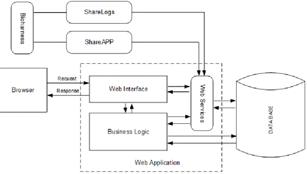
The results obtained in this thesis could have implications both in clinical practice and in clinical research. The system has been designed and developed in order to be clinically feasible. In particular, Heart Rate Variability analysis and the automatic system for identification of high-risk patients are integrated in a web-based platform, developed in the framework of the Smart Health and Artificial Intelligence for Risk estimation (SHARE) project. The platform, now integrated in an open and interoperable cloud
15
computing platform for health and eGovernement (PRISMA), included a standalone software (for Windows operative system) and an Android application to acquire signals from wearable devices. This integration enable to test the clinical feasibility and uptake of the developed tool in a prospective study in subjects aged 55 and over recruited by the Center of Hypertension of the University Hospital of Naples Federico II. Moreover, since 5-minute ECG recording is inexpensive, easy to assess, and non-invasive, future research will focus on the clinical applicability of the system as a screening tool in non-specialized ambulatories (e.g. at General Practitioners’), in order to identify high-risk patients to be shortlisted for more complex (and costly) investigations. Improved identification of individuals at risk for the development of vascular events may result in more targeted and adequate prevention strategies. For example, adopting the model for vascular risk assessment in a cohort of 1000 hypertensive patients, about 200 high risk subjects should be identified, and among them, 80 will develop a vascular event in the following 12 months. Since, as reported by the European Guidelines on cardiovascular disease prevention in clinical practice, most of cardiovascular events could be avoided by changes in life styles and appropriate use of therapeutic treatments, it can be hypotized that the adoption of targeted strategies on the high-risk subjects could halve the number of vascular events.
The findings obtained by the data-mining methods (which did not use any a priori knowledge) reinforce the previous clinical observation that depressed HRV is a marker of cardiovascular risk and, for the first time, showed that it could be also an interesting parameter to be investigated in fall identification and prevention research. In particular, the proposed method does not require the use of other technologies as wearable accelerometers or pressure matrices, which are not used in everyday clinical practices, not having direct benefits for cardiovascular outpatients. For that reason, the method proposed could be used widely in outpatient settings to identify high-risk patients who need further assessment and could benefit from fall prevention programs or fall detection systems.
The main limitation of the achieved findings is the relatively small sample size of the datasets. This issue could be addressed in the next future by increasing the number of enrolled subjects by Center of Hypertension of the University Hospital of Naples Federico II. This would make the present findings clinically more relevant. Moreover, the dataset used in the fall identification issue was not specifically designed to study falls. Therefore, important information, such as the exposure to other independent intrinsic risk factors for falls could not be accessed or used to verify independently the results. Moreover, the fall recordings were based on patient self-reports, which are considered not every time reliable as some non-harmful falls can be forgotten and not reported. Therefore, the number of falls could have been underestimated.
16
Further developments of the current thesis could be the adoption of new Heart Rate Variability measures (e.g. point process time-frequency analysis), strong risk markers extracted from ECG (e.g. Heart Rate Turbulence or T wave alterations), and other non-invasive measures obtained by wearable sensors (e.g accelerometric signals, breath rate).
Outline
The thesis is organized as follows:
in the chapter 1, the main topics which are addressed in the thesis, such as Autonomous Nervous System, Heart Rate Variability, cardiovascular diseases, are briefly introduced;
the adopted databases are described in the Chapter 2;
the adopted methods, including features computation and selection, machine learning algorithms, are reported in Chapter 3;
in the Chapter 4, the main results are presented and discussed in relation with the state of art;
the Chapter 5 provides the conclusions of the works.
17
1 Introduction
1.1 Autonomic Nervous System
The Autonomic Nervous System (ANS) innervates primarily the smooth musculature of all organs, the heart and the glands in order to mediate the neuronal regulation of the internal milieu. (Jänig, 1989) The functions of the ANS are to keep the internal milieu of the body constant or adjust it as required by changing circumstances (e.g. mechanical work, stressful situation, food intake). The actions of ANS are in general not under direct voluntary control. The ANS consists of two subdivisions: the sympathetic and the parasympathetic nervous system.
The nerves of the sympathetic system originate from the intermediate zone of the thoracic and lumbar spinal cord. The axons of these neurons are thin, but many are myelinated; their conduction velocities range from 1 to 20 m/s. They leave the spinal cord in the ventral roots and the white rami communicants, and terminate in the paired paravertebral ganglia or the unpaired paravertebral abdominal ganglia. The paravertebral ganglia are connected by nerve strands to form a chain on either side of the vertebral column. From these sympathetic trunks, the thinner, unmyelinated postganglionic axons either pass in the grey rami to the effectors in the periphery of the body, or form special nerves that supply organs in the head region or in the thorax, abdomen and pelvis.
The cell bodies of the preganglionic parasympathetic neurons are in the sacral cord and the brainstem. All the axons are very long as compared with those of the sympathetic preganglionic neurons. They form special nerves to the parasympathetic postganglionic neurons, which are near or in the effector organs.
The efficacy of the heart as pump is controlled by sympathetic and parasympathetic nerves, which supplied the heart. The parasympathetic nerves (the vagi) are distributed mainly to the sinoatrial and atrioventricular nodes, to a lesser extent to the muscle of the two atria, and very little directly to the ventricular muscle. The sympathetic nerves, conversely, are distributed to all parts of the heart, with strong representation to the ventricular muscle as well as to all the other areas.
Stimulation of the parasympathetic nerves to the heart causes the hormone Acetylcholine to be released at the vagal endings. This hormone has two major effects on the heart. First, it decreases the rate of rhythm of the sinus node, and second, it decreases the excitability of the atrioventricular junctional fibers between the atrial musculature and the atrioventricular node, thereby slowing transmission of the cardiac impulse into the ventricles. Weak to moderate vagal stimulation slows the rate of heart pumping, often to as little as one half normal, and strong stimulation of the vagi can stop completely the rhythmical excitation by the sinus node or block completely transmission of the cardiac impulse from the atria into the ventricles through the atrioventricular mode. In either case,
18
rhythmical excitatory signals are no longer transmitted into the ventricles. The ventricles stop beating for 5 to 20 seconds, but then some point in the Purkinje fibers, usually in the ventricular septal portion of the atrioventricular bundle, develops a rhythm of its own and causes ventricular contraction at a rate of 15 to 40 beats per minute. This phenomenon is called ventricular escape.
The acetylcholine released at the vagal nerve endings greatly increases the permeability of the fiber membranes to potassium ions, which allows rapid leakage of potassium out of the conductive fibers. This causes increased negativity inside the fibers, an effect called hyperpolarization, which makes this excitable tissue much less excitable. In the sinus node, the state of hyperpolarization decreases the “resting” membrane potential of the sinus nodal fibers to a level considerably more negative than usual, to -65 to -75 millivolts rather than the normal level of -55 to -60 millivolts. Therefore, the initial rise of the sinus nodal membrane potential caused by inward sodium and calcium leakage requires much longer to reach the threshold potential for excitation. This greatly slows the rate of rhythmicity of these nodal fibers. If the vagal stimulation is strong enough, it is possible to stop entirely the rhythmical self-excitation of this node. In the atrioventricular node, a state of hyperpolarization caused by vagal stimulation makes it difficult for the small atrial fibers entering the node to generate enough electricity to excite the nodal fibers. Therefore, the safety factor for transmission of the cardiac impulse through the transitional fibers into the atrio-ventricular nodal fibers decreases. A moderate decrease simply delays conduction of the impulse, but a large decrease blocks conduction entirely. Sympathetic stimulation causes essentially the opposite effects on the heart to those caused by vagal stimulation, as follows. First, it increases the rate of sinus nodal discharge. Second, it increases the rate of conduction as well as the level of excitability in all portions of the heart. Third, it increases greatly the force of contraction of all the cardiac musculature, both atrial and ventricular. In short, sympathetic stimulation increases the overall activity of the heart. Maximal stimulation can almost triple the frequency of heartbeat and can increase the strength of heart contraction as much as twofold.
Stimulation of the sympathetic nerves releases the hormone norepinephrine at the sympathetic nerve endings. The precise mechanism by which this hormone acts on cardiac muscle fibers is somewhat unclear, but the belief is that it increases the permeability of the fiber membrane to sodium and calcium ions. In the sinus node, an increase of sodium-calcium permeability causes a more positive resting potential and also causes increased rate of upward drift of the diastolic membrane potential toward the threshold level for self-excitation, thus accelerating self-excitation and, therefore, increasing the heart rate.
In the atrioventricular node and bundles, increased sodium-calcium permeability makes it easier for the action potential to excite each succeeding portion of the conducting fiber
19
bundles, thereby decreasing the conduction time from the atria to the ventricles. The increase in permeability to calcium ions is at least partially responsible for the increase in contractile strength of the cardiac muscle under the influence of sympathetic stimulation, because calcium ions play a powerful role in exciting the contractile process of the myofibrils. (Guyton and Hall, 2006)
1.2 Heart Rate Variability
Heart Rate Variability (HRV) is the variation over time of the period between consecutive heartbeats (RR intervals) (Malik et al., 1996) and is usually extracted from electrocardiographic signal recorded through a non-invasive technique. HRV is commonly used to assess the influence of the ANS on the heart (Malik et al., 1996). HRV is usually extracted by electrocardiographic signals (ECG).
Many measures for assessing HRV have been described in literature, particularly with reference to their discrimination ability between different pathophysiological clinical conditions. In general, HRV measurement could be distinguished in: time-domain, frequency-domain and nonlinear measures.
1.2.1 Time-domain HRV measures
A number of standard statistical time-domain HRV measures have been proposed in literature:
the Standard Deviation of all NN intervals, which is the most simplest variable to calculate, but it is dependent from the length of recording period(Malik et al., 1996);
the standard deviation of the average NN interval calculated over short periods, usually 5 min, which is an estimate of the changes in heart rate due to cycles longer than 5 min(Malik et al., 1996);
the mean of the 5-min standard deviation of the NN interval calculated over 24 h, which measures the variability due to cycles shorter than 5 min(Malik et al., 1996);
the square root of the mean squared differences of successive NN intervals(Malik et al., 1996);
the number of times in which the change in successive normal sinus (NN) intervals exceeds 50 ms (Ewing et al., 1984);
percentage of differences between adjacent NN intervals that are longer than 50 ms (pNN50) (Bigger et al., 1988);
the other measures of the pNNx familiy, where the threshold measure x is set to value different from 50 ms (Mietus et al., 2002).
20
Other time-domain measures are based on geometric methods, which can follow one of the following approaches:
a basic measurement of the geometric pattern (e.g. the width of the distribution histogram at the specified level) is converted into the measure of HRV;
the geometric pattern is interpolated by a mathematically defined shape (e.g. approximation of the distribution histogram by a triangle, or approximation of the differential histogram by an exponential curve) and then the parameters of this mathematical shape are used,
the geometric shape is classified into several pattern-based categories which represent different classes of HRV (e.g. elliptic, linear and triangular shapes of Lorenz plots) (Malik et al., 1996).
The most common geometric measures are the following ones:
the HRV triangular index, i.e. the integral of the density distribution (computed as the number of all NN intervals) divided by the maximum of the density distribution of NN intervals(Malik et al., 1996).
the baseline width of the distribution measured as a base of a triangle, approximating the NN interval distribution (the minimum square difference is used to find such a triangle) (Malik et al., 1996).
1.2.2 Frequency-domain HRV measures
The frequency-domain HRV measures rely on the estimation of power spectral density (PSD). Several spectral methods have been applied for the PSD estimation and are usually distinguished in non-parametric and parametric. (Malik et al., 1996) The non-parametric method are based in most of the cases on the Fast Fourier Transform FFT and their advantages are: the simplicity of the algorithm employed and the high processing speed, but they suffer from spectral leakage effects due to windowing. The spectral leakage leads to masking of weak signal that are present in the data. The parametric methods (i.e. model based) avoid the problem of leakage and provide smoother spectral components which can be distinguished independently of preselected frequency bands, easy post-processing of the spectrum with an automatic calculation of low and high frequency power components and easy identification of the central frequency of each component, and an accurate estimation of PSD even on a small number of samples on which the signal is supposed to maintain stationarity. (Malik et al., 1996) The widely used parametric methods is the Autoregressive (AR) model. In AR method, the estimation of AR parameters can be done easily by solving linear equations. In AR method, data can be modeled as output of a causal, all pole, discrete filter whose input is white noise(Acharya et al., 2006) Formally, AR model is expressed by the following equation:
21
𝑥(𝑘) = − ∑ 𝑎(𝑛)𝑥(𝑘 − 𝑛) + 𝑤(𝑘)
𝑁
𝑛=1
where a(n) is AR coefficient and w(k) is white noise of σ2 variance and N is the order of
the model. The parameters of the model are the AR coefficient and the variance σ2. The
most relevant issue related to PSD estimation by AR model is the selection of the order N. Different studies investigated this issue, particularly, by using the Akaike information criteria, enabling to conclude that the model order could be set to 16. (Boardman et al., 2002).
Three main spectral components are distinguished in a spectrum calculated from short-term recordings (2 – 5 minutes): very low frequency (VLF), low frequency (LF), and high frequency (HF) components(Akselrod et al., 1981). Spectral analysis may also be used to analyse the sequence in the entire 24-h period. The result then includes an ultra-low frequency component (ULF), in addition to VLF, LF and HF components. (Malik et al., 1996)
Moreover, the use of techniques such as the FFT require an evenly sampled time series. Since HRV is calculated from the variations in the RR interval series which are inherently irregularly spaced in time, in order to produce an evenly sampled time series prior to FFT-based spectral estimation, linear or cubic spline resampling is usually employed.(Laguna et al., 1998). Ectopic beats, arrhythmic events, missing data and noise effects may alter the estimation of the PSD of HRV. Proper interpolation (or linear regression or similar algorithms) on preceding/successive beats on the HRV signals or on its autocorrelation function may reduce this error(Malik et al., 1996). A recent study(Clifford and Tarassenko, 2005) showed that Lomb-Scamble periodgram, a more appropriate spectral estimation technique for unevenly sampled time series that uses only the original data,(Lomb, 1976) provides a superior PSD estimate of RR series compared to FFT techniques, with reference to ectopic beat removal or replacement.
1.2.3 Nonlinear HRV measures
Recent developments in the theory of nonlinear dynamics have paved the way for analysing signals generated from nonlinear living systems(Acharya et al., 2006). It is now generally recognized that these nonlinear techniques are able to describe the processes generated by biological systems in a more effective way. The most common nonlinear techniques applied to HRV analysis are: Poincaré Plot(Brennan et al., 2001), Approximate Entropy(Richman and Moorman, 2000), Sample Entropy(Richman and Moorman, 2000), Correlation Dimension(Carvajal et al., 2005), Detrended Fluctuation Analysis(Peng et al., 1995a, Penzel et al., 2003), and Recurrence Plot (Trulla et al., 1996, Webber and Zbilut, 1994, Zbilut et al., 2002).
22
1.2.3.1 Poincaré Plot
The Poincaré Plot, also known as return map, is a common graphical representation in which each point is represented as a function of the previous one. In HRV analysis, Poincaré Plot is the scatterplot of the successive RR versus previous one. A widely used approach to analyse the Poincaré plot of RR series consists in fitting an ellipse oriented according to the line-of-identity and computing the standard deviation of the points perpendicular to and along the line-of-identity referred as SD1 and SD2, respectively(Brennan et al., 2001).
It has been shown that SD1 and SD2 are related to linear measures of HRV(Brennan et al.,
2001). Moreover, the two Poincaré Plot measures are related to the autocovariance function and, for that reason, these two Poincaré Plot measures could not provide independent nonlinear information and in recent review on HRV(Rajendra Acharya et al., 2006) they are discussed in the standard time domain analysis instead of nonlinear methods. Two kind of generalization of the Poincaré Plot are proposed in the literature(Brennan et al., 2001): the lagged Poincaré Plot and the higher order Poincaré Plot.
The lagged Poincaré Plot is the plot of RRn+m against RRn where m is chosen from 2 to
some small positive value (not higher than 8). SD1 and SD2 are computed similarly as lag
m set to 1 and are also related to the autocovariance function. For that reason, the set of
lagged Poincaré Plot is a description of the autocovariance function.
Poincaré Plot of order m is a m-dimensional scatter-plot of the m-ples (RRn, RRn+1,…,
RRn+m). This plot resulted in 2-dimensional projection into each of the coordinate planes
(RRn, RRn+1), (RRn+1, RRn+2),…,(RRn, RRn+m). The first two projections are equivalent to
standard Poincaré Plot, the last one is equivalent to a Poincaré Plot with lag m, and the other projections are equivalent to Poincaré Plot with lag up to m. In other words, an order
m Poincaré Plot is geometrically described by a set of Poincaré Plot with lag up to m+1.
Geometrically, SD1 measures the width of the Poincaré cloud and, therefore, indicates the
level of short-term HRV, while SD2 measures the length of the cloud along the
line-of-identity, reflecting the long-term HRV. Mathematically, the findings by Brennan et al. (Brennan et al., 2001) proposed the interpretation of SD1 as a measure of short-term (over each beat) variability, and of SD2 as a measure of the difference between total variability and short-term variability. This could be explained by considering a time series which shows variability only over a single beat, such as a sequence alternating between two value (RRI, RRII, RRI, RRII,…,RRI, RRII). The Poincaré Plot of this series shows a zero
length and zero value of SD2, which are coherent with the absence of long-term
variability, while the SD1 has a non-zero value, reflecting the short-term variability of the
23
Others techniques, such as central tendency measure(Hnatkova et al., 1995), density based approach(Cohen et al., 1996), have been applied in order to extract independent nonlinear information from Poincaré Plot, but they are not as widely used as SD1 and
SD2.
1.2.3.2 Approximate entropy
Approximate entropy (AppEn) is widely used method to measure the complexity of signal(Pincus, 1991). It shows the probability that similar observation patterns do not repeat. If a time series demonstrates complex, irregular behaviour, than it will have a high
AppEn values. For instance, sinusoids give approximately zero value of AppEn. AppEn
showed several advantages: it can be applied for both short-term and long-term recordings, it is scale invariant, model independent, easy to use and it is able to discriminate time series for which clear future recognition is difficult(Rajendra Acharya et al., 2006, Chon et al., 2009). For that reason, it has been applied in different fields, particularly in cardiovascular signal analysis to assess the irregularity of the RR series(Richman and Moorman, 2000).
The AppEn computation rely on the values of two parameters: m, the embedding dimension, and r, the tolerance threshold, which are required to be specified a priori. Several clinical studies(Pincus, 1991, Niskanen et al., 2004, Ho et al., 1997) have shown that either m=1 or 2 and r between 0.1 and 0.2 times the SDNN are suitable to provide valid value of AppEn. However, a recent study(Chon et al., 2009) recommended the use of the r value (rmax) which maximizes the AppEn (AppEnmax). This conclusion was derived
by the observation that the AppEn computed with value of r within the recommended range 0.1 - 0.2 provided misleading results in simulated signals. The AppEn determines the conditional probability of similarity between a chosen data segment of a given duration and the next segment set of the same duration; the higher the probability the smaller the AppEn value, reflecting less complexity. Applying AppEn to the following three time series with decreasing complexity: white noise, cross chirp, and sinusoidal signals, AppEnmax provides higher values for white noise, then for cross chirp and lower
value for sinusoidal signals, according to their decreasing complexity. If other values of
r threshold are adopted, misleading results can arise, such as higher values for cross chirp
than for white noise. Moreover, a previous study on human HRV data (Castiglioni and Di Rienzo, 2008) showed that a selection of r=0.25 resulted in a 12% decrease of AppEn values, whereas r=0.1 results in 9% increase as subjects changed their body position from supine to upright. The AppEnmax denotes the largest information difference between data
length m and m+1 for any given r, reflecting the maximum complexity. However, the choice of AppEnmax is a computation burden and in order to avoid the computation of
AppEn for each possible r value to find the maximum value, nonlinear models were
proposed and validated to estimate rmax value from variability of the signals. In particular,
for m=2, Chon et al.(Chon et al., 2009) proposed an empirical formula. However, a recent study by Liu(Liu et al., 2011) aimed to verify whether Chon’s method was appropriate
24
for HRV by comparing AppEn in two groups: healthy subject and patients suffering from cardiac disease. AppEn value were computed with three different value of the thresholdr : SDNN r0.2* (AppEn0.2); max r r ; chon r r (AppEnChon).
Surprisingly, only AppEnChon (not AppEn0.2 nor AppEnmax) was statistically different
between the two groups. Another recent study analysed the three different type of AppEn in healthy subjects under stress compared to controlled resting condition(Melillo et al., 2011a). Also in this study, AppEnmax was not statistically different between the two
groups, while statistically significant differences were observed in AppEn0.2 e AppEnChon.
The findings of these studies could be explained according to the analysis of the Chon’s empirical formula, particularly, its relationship with the ratio between short-term and long-term variability. Further studies should focus on development of methods which can reduce the influence from the different threshold values r in AppEn computation. 1.2.3.3 Sample entropy
Sample Entropy (SampEn) is a relatively new feature introduced by Richman et al.(Richman and Moorman, 2000) to measure the complexity and the regularity of clinical time series. It is very similar to AppEn, with some important differences in its calculation.
SampEn, in theory, does not depend on the length of the time series, but it also relies on
the choice of the parameters m and r, such as AppEn. However, the dependence on the parameter r is different: SampEn decreases monotonically when r increases. With high value of N and r, SampEn and AppEn provide comparable results(Rajendra Acharya et al., 2006), for that reason, the applications of the two measures are very similar.
1.2.3.4 Fractal Dimension, Correlation Dimension and Detrended Fluctuation Analysis The term “fractal” was first defined as a geometric concept(Mandelbrot, 1982), referring to an object satisfying two properties: self-similarity and fractional dimensionality. The former property means that an object is composed of subunits (and sub-subunits on multiple levels) that statically resemble the structure of the whole object. The latter property means that the object has a fractional dimension. For example, in bidimensional curve, to verify self-similarity, a subset of the object is rescaled to the same size of the original object, using the same magnification factor for both its width and height, and its statistical properties are compared with those of the original object. Mathematically, this property should hold on all scales, however, in the real world, there are necessarily lower and upper bounds over which such self-similar behaviour applies. Moreover, the strict criterion requires that all the statistical properties (including all higher moments) are identical. Therefore, in practice, a weaker criterion is adopted by examining only the
25
means and variances (first and second moments) of the distribution. The second criteria distinguishes fractal from Euclidean objects, which have integer dimension. For example, a square satisfies self-similarity as it can be divided into smaller subunits that resemble the large square, but it is not a fractal since it has an integer (2) dimension. Fractal-like appearance was observed in several cardiovascular structures, such as the arterial and venous tree and His-Purkinje network.
The concept of fractal has been extended to the analysis of time series. For instance, in order to verify self-similarity in time series, a subset of the time series is selected and rescaled, but with two different magnification factors (since the two axes have independent physical units). Mathematically, a time series is self-similar if
𝑥(𝑡) ≡ 𝑎𝑎𝑥 (𝑡
𝑎)
where a is the self-similarity parameter or scaling exponent and the operator ≡ indicate that the statistical properties of both side of the equation are identical; however, as already stated, in practice, only the first and second moment statistical properties are compared. The scaling exponent could be estimated by Detrended Fluctuation Analysis, while the Higuchi’s algorithm could be adopted for estimation of the fractal dimension (FD)(Higuchi, 1988). The correlation dimension CD is one of the most widely used measures of the fractal dimension and has been adopted to measure the complexity for the HRV time series(Carvajal et al., 2005).
Detrended Fluctuation Analysis is used to quantify the fractal scaling properties of short
RR time series, by measuring the correlation within the signal(Penzel et al., 2003, Peng
et al., 1995a). It is a modified version of root-mean-square analysis of random walks(Huikuri et al., 2000) and consists into: integration of the root-mean-square fluctuation, computation of detrended time series at observation window of different size and plot against the windows sizes on a log-log scale and the scaling exponent α is computed the slope of the regression line. The value of α for white noise, for fractal-like signal and Brownian noise (integral of Gaussian noise) are 0.5, 1 and 1.5, respectively(Huikuri et al., 2000, Ho et al., 1997). In HRV analysis, other two additional indexes are usually computed(Schulz et al., 2010, Peng et al., 1995b): short-term fluctuations (Alpha1) and long-term fluctuations (Alpha2).
1.2.3.5 Recurrence Plot
Recurrence Plot was introduced by Eckmann et al.(Eckmann et al., 1987) as a graphical tool to discover hidden periodicities, difficult to be detected otherwise, and can be used to reveal non-stationarity in the time series. The recurrence plot is an array of dots in an
N x N square, where a dot is placed at (i,j) whenever RRj is sufficiently close to RRi. The
plots will be symmetric along the diagonal i = j, because if RRi is close to RRj, then RRj
26
indicating more variation indicating high variation in the heart rate. Abnormalities like ischemic/dilated cardiomyopathy cases, show more squares in the plot indicating the inherent periodicity and the lower heart rate variation(Acharya et al., 2006).
1.3 Congestive Heart Failure
Congestive Heart Failure (CHF) is a patho-physiological condition due to an abnormal cardiac function, which is responsible for the failure of the heart to pump blood as required by the body. It is a common end-stage of heart disease, greatly shortening survival. CHF is associated with profound derangements of the ANS, which worsen disease progression(Cohn, 1990). Sympathetic tone is markedly increased while parasympathetic modulation of heart rate is markedly decreased(Floras, 1993). Hemodynamic and metabolic abnormalities probably serve as the afferent stimulus for this response. This chronic activation is accompanied by an attenuation of reflex responsiveness to unloading of the central baroreceptors and mechanoreceptors. Loss of the buffering capacity of these afferent receptors may contribute to the sustained sympathetic stimulation. The renin-angiotensin system is uncoupled from the sympathetic nerves, probably because the intrarenal mechanisms subserving renin release are preserved. Chronic activation of the sympathetic nerves may contribute to disturbed hemodynamics as well as to long-term structural changes that may influence the natural history of the disease. (Cohn, 1990)
CHF severity can be measured with the symptomatic classification scale of the New York Heart Association (NYHA) (Fleg et al., 2000). Classification via NYHA scale has been proved to be a risk factor for mortality (Redfield et al., 1998, Gheorghiade et al., 2005). NYHA functional classification identifies patients in one of four categories based on physical symptoms and activity restriction:
Class I – No symptoms with ordinary activity. No limitations on activity
Class II – Slight to moderate symptoms with normal activity. Slight limitation of activity.
Class III – Moderate symptoms with less than normal activity. Marked limitation of activity.
Class IV – Inability to carry out any physical activity without discomfort. Symptoms may occur at rest(Carels, 2004).
1.4 Hypertension and risk assessment
Hypertension is the most common cardiovascular disease. Hypertension is defined as values higher than 140mmHg for systolic blood pressure and/or higher than 90mmHg for diastolic blood pressure. Limited comparable data are available on the prevalence of hypertension and the temporal trends of blood pressure values in different European
27
countries(Pereira et al., 2009). Overall, the prevalence of hypertension appears to be around 30–45% of the general population, with a steep increase with ageing.
1.4.1 Cardiovascular risk estimation
Estimation of total cardiovascular risk is easy in particular subgroups of patients, such as those with antecedents of established cardiovascular disease, diabetes, or with severely elevated single risk factors. In all of these conditions, the total cardiovascular risk is high or very high, calling for intensive cardiovascular risk-reducing measures. However, a large number of patients with hypertension do not belong to any of the above categories and the identification of those at low, moderate, high or very high risk requires the use of models to estimate total cardiovascular risk, so as to be able to adjust the therapeutic approach accordingly.
Several risk estimation system have been developed(Pyorala et al., 1994, D'Agostino et al., 2008, Conroy et al., 2003, Woodward et al., 2007, Hippisley-Cox et al., 2008, Assmann et al., 2002, Ridker et al., 2008, Ridker et al., 2007) and their values and limitations have been reviewed recently(Cooney et al., 2009). Most of the current risk estimation systems include the conventional risk factors: age, sex, smoking, blood pressure, and lipid levels. Recently, there has also been increasing interest in the inclusion of family history of chronic heart disease (Woodward et al., 2007, Hippisley-Cox et al., 2008, Ridker et al., 2008, Ridker et al., 2007), social deprivation measures (Woodward et al., 2007, Hippisley-Cox et al., 2008), ethnicity(Hippisley-Cox et al., 2008), and interaction variables that adjust for the use of antihypertensive medication (Woodward et al., 2007, Hippisley-Cox et al., 2008, Wilson et al., 1998).
Most of the current risk estimation systems are based on proportional hazards models, such as Cox (semiparametric) or Weibull (parametric). The Cox method has the advantage of not making any assumptions regarding the shape of the underlying survival, in contrast to the Weibull method, which imposes a parametric function on the baseline survival. One limitation of all risk estimation systems is that they assume constant effects of the risk factors at differing ages and levels of the other risk factors. One system (QRISK2) has attempted to overcome the problem of differing effects of the risk factors with increasing age by including interaction variables between age and several of the other risk factors(Hippisley-Cox et al., 2008). However, this method still assumes that the interaction effect with age remains constant at all ages. Certain combinations of risk factors may act synergistically to increase risk in a manner that is more than additive. Some data-mining methods, such as cluster analysis, neural networks and tree-based algorithm, attempt to account for this. These methods are particularly useful for selecting the most appropriate variables when a large number of potential predictors of risk are available. Neural networks do not assume that risk factors function in a constant and continuous fashion and can account for complex nonlinear relationships and interactions between risk factors. Cluster analysis focuses on the identification of groups of persons
28
with similar risk factor characteristics who have similar levels of risk. Tree-based algorithms attempt to progressively split the population into smaller subgroups, through sequential introduction of the risk factors, starting with the simplest. The advantage is that some persons can be classified as high or low risk based on very few risk factors, reducing unnecessary laboratory testing for them. However, these methods introduce other problems. The main problem with all of these methods is model shrinkage, that is, their predictive ability declines sharply once the model is applied to an external dataset, which limits their utility in clinical practice. Moreover, there is difficulty in obtaining large epidemiological datasets with extensive numbers of predictor variables available. Additionally, the necessity for measurement of multiple factors in clinical practice adds to complexity and is, therefore, likely to limit clinical usage of these systems.
1.4.2 Fall risk
Falls represent one of the most common causes of injury-related morbidity and mortality in later life. The consequences of falls range from psychological harm, through serious physical injuries (Lord et al., 2006) and hospitalization, to death (Rubenstein, 2006), often causing a reduction of independence in the faller. Falls reduce overall well-being, mobility and quality of life, of individuals and families (Katz and Shah, 2010). The mean and median costs of a fall is about 9,000 and 11,000 euro (Siracuse et al., 2012). Over 400 risk factors for falls have been identified and classified as either extrinsic, such as environment and circumstances, or intrinsic, which include deterioration of neurological functioning and sensory and/or cardiovascular impairments. The prioritization of those risk factors remains unclear and the sensitivity, specificity and applicability of subject-specific assessment of fall risk remains imprecise (Pecchia et al., 2011, Gates et al., 2008).
Only 31% of falls appear to be due to accidents (Rubenstein, 2006) and also those accidental falls may be due to complex and dynamic unrevealed interactions between intrinsic and extrinsic risk factors (guidelines, 2013). According to Rubens(Rubenstein, 2006), 42% of falls are due to transient problems, including: gait/balance disorders or weakness (17%), dizziness/vertigo (13%), drop attacks (9%), postural hypotension (3%). For that reason, ANS disturbance and cardiovascular disorders including carotid sinus hypersensitivity, serious arrhythmias, severe valvular heart disease, and coronary heart disease may be underestimated causes of falls(Isik et al., 2012).
Several test have been developed for assessing mobility, some of which have also been suggested as predictor of falls(Tiedemann et al., 2008):
Sit-to-stand test: this test is used as a measure of lower limb strength (Csuka and McCarty, 1985) and is included in fall risk assessment scales(Tinetti, 1986, Berg et al., 1992, Smith, 1994). For the sit-to-stand test with five repetitions (STS-5),
29
subjects were asked to rise from a standard height (43 cm) chair without armrests, five times, as fast as possible with their arms folded. Subjects undertook the test barefoot and performance was measured in seconds, as the time from the initial seated position to the final seated position after completing five stands. The single sit-to-stand task (time from sitting to standing) (STS-1) was also evaluated as it has been used in assessment scales(Berg et al., 1992, Judge et al., 1996) as a measure of functional mobility, balance and lower limb strength.
Pick-up-weight test: The ability to reach down and pick up an object from the floor has been included in several mobility assessment scales (Berg et al., 1992, Reuben and Siu, 1990). A bag containing a 5 kg weight with handles that extended 50 cm above the floor was placed on the floor in front of the subject. The subjects were asked to pick up the bag and place it on a table using one hand only. Performance was rated as either able or unable to complete the task.
Half-turn test: The ability to turn around in an efficient manner has been included in assessments of mobility and balance in older people(Berg et al., 1992, Podsiadlo and Richardson, 1991). Subjects were asked to take a few steps and then turn around to face the opposite direction. The number of steps taken to complete this 180° turn was counted.
Alternate-step test: The alternate-step test (AST) is a modified version of the Berg stool-stepping task(Berg et al., 1992). It involves weight shifting and provides a measure of lateral stability. This test involved alternatively placing the entire left and right feet (shoes removed) as fast as possible onto a step that was 18 cm high and 40 cm deep. The time taken to complete eight steps, alternating between the left and right feet comprised the test measure.
Six-metre-walk: Slow gait speed is associated with an increased risk of falls (Imms and Edholm, 1981, Bootsma-van der Wiel et al., 2002) and is a measure included in fall risk assessment scales (Podsiadlo and Richardson, 1991, Piotrowski and Cole, 1994). Subjects completed a six-metre-walk test (SMWT) measured in seconds along a corridor at their normal walking speed. A 2-m approach and a further 2 m beyond the measured 6-m distance ensured that walking speed was constant across the 6 m.
Stair ascent and descent: The inability to negotiate stairs is a marker of functional decline in older people (Guralnik et al., 1994) and many falls occur during this task(Facts, 1996). The test stairs were indoors, had a handrail, were covered with linoleum and well lit. The subjects started the stair-ascent test at the bottom of eight steps (15 cm high, 27.5 cm deep). Subjects could use the handrail if preferred and a walking aid if they normally used one. Timing commenced for the stair-ascent test when the subject raised their foot off the ground to climb the first step and stopped when both feet were placed on the eighth step (which was a landing). After a brief rest, the subject was asked to descend the stairs. Timing was started when they raised their foot off the ground for the first step and stopped when they
30
completed the last step. Time taken to complete the ascent and descent tests was recorded.
A recent study (Tiedemann et al., 2008) compared these functional tests and showed that, when dichotomised, the AST was the best test for discriminating between the faller groups. An AST cut-off point of 10 s was associated with a 130% increased risk, with 69% sensitivity and 56% specificity with respect to identifying multiple fallers. At identified cut-off points, the STS-5 (12 s), the SMWT (6 s), the stair-descent test (5 s) and the stair-ascent test (5 s) could also significantly predict subjects who suffered multiple falls with sensitivities and specificities above 50%.
31
2 Databases
In the current chapter, the characteristics of the ECG holter databases that have been used for this thesis work are presented. Table 2.1 reported the summary properties of each database that will be then detailed in the following sections.
Table 2.1 Summary of the adopted database
Database Number of subjects Clinical Condition Availability
Congestive Heart Failure
RR Interval Database 29 (aged 34 to 79; 8 male, 2 female) CHF
www.physionet.org
(PhysioBank: Public data archives) BIDMC Congestive Heart
Failure Database.
15 (aged 22 to 71;
11 male, 4 female) CHF
www.physionet.org
(PhysioBank: Public data archives) ECG Holter database
for Vascular Events 139 (age: 72 ± 7 years; 90 male, 49 female) without vascular events Hypertension with or
www.physionet.org
(PhysioNetWorks, for registered users) ECG Holter database
for Fall Risk
168 (age: 72 ± 8 years; 108 male, 60 female)
Hypertension with or without history of fall
progettoshare.it (by request)
2.1 Congestive Heart Failure Holter databases
2.1.1 Background and rationale
For the investigation of ECG holter in CHF patients, two databases are freely available from physionet.org(Goldberger et al., 2000):
Congestive Heart Failure RR Interval Database BIDMC Congestive Heart Failure Database.
2.1.2 Population
The Congestive Heart Failure RR Interval Database provides the RR time-series for 29 long-term ECG recordings of subjects aged 34 to 79, with CHF (NYHA classes I, II, and III). Subjects included 8 men and 2 women; gender is not known for the remaining 21 subjects. The BIDMC Congestive Heart Failure Database includes long-term ECG recordings from 15 subjects (11 men, aged 22 to 71, and 4 women, aged 54 to 63) with severe congestive heart failure (NYHA class 3-4).
2.1.3 Protocol and measurement system
The original ECG recordings, even if are not available, of the Congestive Heart Failure RR Interval Database were digitized at 128 samples per second, and the beat annotations were obtained by automated analysis with manual review and correction. The database is contributed by Rochelle Goldsmith, of Columbia-Presbyterian Medical Center, New York. The individual recordings of the BIDMC Congestive Heart Failure Database are each about 20 hours in duration, and contain two ECG signals each sampled at 250 samples per second with 12-bit resolution over a range of ±10 millivolts. The original
32
analog recordings were made at Boston's Beth Israel Hospital (now the Beth Israel Deaconess Medical Center) using ambulatory ECG recorders with a typical recording bandwidth of approximately 0.1 Hz to 40 Hz. The RR time-series were obtained using an automated detector (without manual review and correction)
2.2 ECG Holter database for Vascular Events
2.2.1 Background and rationale
Previous studies showed that HRV could be an independent risk factor for vascular events: Sajadieh et al. showed that subjects with familial predisposition to premature heart attack and sudden death have reduced HRV(Sajadieh et al., 2003); Dekker et al. concluded that low HRV is associated with increased risk of coronary heart disease and death from several causes (Dekker et al., 2000). Binici et al. demonstrated that depressed nocturnal heart rate variability is a strong marker for the development of stroke in apparently healthy subject (Binici et al., 2011). Since hypertension is a risk factor for vascular events and to the best of authors’ knowledge, no public database of hypertensive patients with a follow-up after the recording is freely available, a database of ECG holter recorded in hypertensive patients were collected ad hoc in order to investigate future vascular events in a twelve month follow-up.
2.2.2 Population
The records have been collected among the hypertensive patients aged 55 or over, followed up by the outpatient hypertension centre of the University Hospital of Naples Federico II. The recordings have been performed between 1 January 2012 and 10 November 2012.
The following exclusion criteria have been adopted: refusal of written informed consent;
severe ocular disease;
deafness in alone living subject;
chronic obstructive pulmonary disease, (pre)dementia, or other disease which may reduce life expectancy.
The dataset consists of 139 hypertensive patients (including 49 female and 90 male, age 72 ± 7 years). Clinical and demographic features of the included subjects are reported in Table 2.2. Among the study sample, in the 12-month follow-up after recordings, 17 patients experienced a recorded event (11 myocardial infarctions, 3 strokes, 3 syncopal events) and for that reason, were considered as high-risk subjects, while the remaining ones as low-risk subjects.
33
Table 2.2 Clinical and demographic feature of the subjects included in the ECG Holter database for Vascular Events
ID Sex Age Weight Height BSA1 BMI2 Smoker F hyp3 F stroke4 SP5 DP6 IMT7 LVMi8 EF9 Vascular event
1911 M 56 105 180 2.29 32.41 yes no no 140 80 4 123 66 none 2012 M 72 83 169 1.97 29.06 no no no 130 75 n/a 121 69 none 2019 F 80 80 165 1.91 29.38 no no no 177 75 2.5 164 56 none 2020 M 77 88 178 2.09 27.77 no no no 140 85 2.7 115 67 none 2025 F 66 80 174 1.97 26.42 no no no 110 65 1.5 98 66 none 2031 M 84 72 170 1.84 24.91 no no no 120 70 2.6 147 51 none 2032 F 66 85 160 1.94 33.20 no no no 150 65 1.6 178 53 none 2033 M 77 82 169 1.96 28.71 no no yes 115 80 n/a 144 42 myocardial infarction 2035 M 77 80 162 1.90 30.48 no yes yes 160 75 n/a 123 70 none 2037 F 69 90 154 1.96 37.95 no yes no 110 65 1.5 124 64 none 2041 M 85 97 165 2.11 35.63 no no no 135 75 3 159 50 none 2047 F 69 83 173 2.00 27.73 no no no 146 80 1.9 86 68 none 2050 M 73 68 167 1.78 24.38 no yes no 105 70 1.7 202 43 none 2055 M 65 72 167 1.83 25.82 no no no 130 85 2.3 106 68 none 2057 F 66 72 176 1.88 23.24 no yes no 130 85 2 117 66 none 2059 F 75 80 150 1.83 35.56 no no no 170 80 n/a 154 71 myocardial infarction 2062 M 72 93 187 2.20 26.59 no no no 120 80 1.4 126 65 none 2063 M 70 82 178 2.01 25.88 no yes no 162 100 1.6 153 62 none 2065 F 69 81 170 1.96 28.03 no yes yes 135 65 2.7 105 66 none
1 Body surface area 2 Body Mass index
3 Family history of hypertension 4 Family history of stroke 5 Systolic arterial pressure 6 Diastolic arterial pressure 7 Intima media thickness 8 Left ventricular mass index 9 Ejection fraction
34
ID Sex Age Weight Height BSA1 BMI2 Smoker F hyp3 F stroke4 SP5 DP6 IMT7 LVMi8 EF9 Vascular event
2066 M 74 74 165 1.84 27.18 no no no 130 80 3.1 121 63 none 2068 M 67 72 171 1.85 24.62 yes yes no 120 85 n/a 144 61 none 2069 M 64 86 178 2.06 27.14 no no no 115 75 2.2 111 61 none 2072 M 73 64 174 1.76 21.14 yes no no 125 75 1.2 119 67 none 2073 M 73 60 167 1.67 21.51 no no no 195 95 2.4 141 32 none 2076 M 68 62 165 1.69 22.77 yes no no 143 62 3.7 168 33 none 2078 M 74 85 180 2.06 26.23 yes yes no 150 75 1.7 140 67 none 2079 M 71 113 168 2.30 40.04 no no no 150 85 2.6 156 67 none 2082 M 58 92 175 2.11 30.04 yes yes no 135 70 1.6 98 69 none 2084 F 70 93 165 2.06 34.16 no yes no 140 70 2.2 n/a n/a none 2087 F 71 74 172 1.88 25.01 no yes no 160 75 2.3 126 65 none 2089 F 75 68 156 1.72 27.94 yes no no 135 65 1.7 93 64 none 2092 F 73 98 170 2.15 33.91 no yes no 155 78 2.9 129 65 none 2097 M 79 81 172 1.97 27.38 yes no no 110 80 2.4 125 46 none 2100 F 64 83 155 1.89 34.55 yes no no 200 80 3.3 156 62 none 2102 M 74 74 172 1.88 25.01 no yes no 150 90 n/a n/a n/a none 2107 M 76 70 160 1.76 27.34 no yes yes 145 75 3 146 60 none 2108 M 84 70 170 1.82 24.22 yes no no 164 54 3.5 194 63 myocardial infarction 2114 F 72 55 160 1.56 21.48 yes yes no 160 80 3 99 65 none 2115 M 75 75 172 1.89 25.35 yes no no 122 74 3.3 121 68 none 2116 M 65 98 171 2.16 33.51 no no no 130 80 1.7 125 54 none 2117 M 69 65 175 1.78 21.22 no yes no 140 80 2.3 113 38 none 2119 F 74 91 162 2.02 34.67 no no no 140 80 2.3 101 72 stroke 2120 F 81 76 158 1.83 30.44 no yes no 160 80 2 163 66 none 2121 M 81 93 170 2.10 32.18 yes no no 170 75 5 159 62 myocardial infarction 2125 F 72 78 158 1.85 31.24 no yes no 190 80 4.2 154 72 none 2134 F 86 78 160 1.86 30.47 no yes no 145 55 2.2 122 59 none 2136 M 77 84 173 2.01 28.07 no no yes 155 85 2 154 66 none
35
ID Sex Age Weight Height BSA1 BMI2 Smoker F hyp3 F stroke4 SP5 DP6 IMT7 LVMi8 EF9 Vascular event
2139 M 64 75 165 1.85 27.55 no no no 140 90 2.1 113 64 none 2140 M 70 91 187 2.17 26.02 no no no 145 85 2.3 127 65 none 2142 M 71 80 160 1.89 31.25 no no yes 165 80 3.3 152 53 none 2148 F 66 64 156 1.67 26.30 no no no 130 75 2 129 60 myocardial infarction 2150 M 59 68 164 1.76 25.28 yes no yes 100 60 1.4 98 69 none 2152 F 82 64 156 1.67 26.30 no no no 110 70 1.6 159 65 none 2154 M 80 75 167 1.87 26.89 yes no no 105 65 2.3 117 52 none 2156 M 69 80 165 1.91 29.38 yes no no 150 90 2.5 n/a n/a none 2159 M 75 68 169 1.79 23.81 no yes no 160 90 2.7 107 70 none 2161 M 74 78 166 1.90 28.31 no yes no 130 70 2.4 122 56 none 2167 M 77 80 169 1.94 28.01 yes no no 170 70 3 128 62 none 2168 M 83 75 170 1.88 25.95 no no no 145 70 3.3 129 58 none 2170 F 65 59 154 1.59 24.88 no no no 145 65 1.8 n/a n/a none 2171 M 77 89 163 2.01 33.50 no no no 125 80 1 118 69 none 2175 M 69 75 169 1.88 26.26 yes no no 150 86 2.2 n/a n/a none 2180 M 69 88 171 2.04 30.09 no yes no 120 70 1.7 133 62 none 2184 F 68 55 165 1.59 20.20 no yes no 110 70 1.35 98 68 myocardial infarction 2185 M 81 72 171 1.85 24.62 yes yes no 145 80 2.9 148 60 myocardial infarction 2186 F 65 67 159 1.72 26.50 no yes no 135 75 3.6 116 73 none 2188 F 85 75 160 1.83 29.30 no no no 130 80 3.5 131 36 none 2191 M 73 92 173 2.10 30.74 no yes yes 155 85 3.6 139 52 none 2194 F 68 95 162 2.07 36.20 no yes no 145 75 1.8 118 72 none 2202 M 63 72 168 1.83 25.51 no yes yes 135 85 1.4 n/a n/a none 2210 F 80 58 153 1.57 24.78 no no no nan nan n/a n/a n/a none 2213 M 65 82 175 2.00 26.78 no yes no 120 80 2.5 154 56 none 2215 m 92 62 165 1.69 22.77 no no no 120 80 3 126 57 none 2218 F 77 64 160 1.69 25.00 no yes no 110 60 1.5 146 70 syncope 2219 F 75 72 162 1.80 27.43 no no no 150 75 1.4 149 45 none