fluid-structure interaction problems
Francesco Ballarin, Gianluigi Rozza and Yvon Maday
Abstract POD–Galerkin reduced-order models (ROMs) for fluid-structure interaction problems (incompressible fluid and thin structure) are proposed in this paper. Both the high-fidelity and reduced-order methods are based on a Chorin-Temam operator-splitting approach. Two different reduced-order methods are proposed, which differ on velocity continuity condition, imposed weakly or strongly, respectively. The resulting ROMs are tested and com-pared on a representative haemodynamics test case characterized by wave propagation, in order to assess the capabilities of the proposed strategies.
1 Introduction
Several applications are characterized by multi-physics phenomena, such as the interaction between an incompressible fluid and a compressible structure. The capability to perform real-time multi-physics simulations could greatly increase the applicability of computational methods in applied sciences and engineering. To reach this goal, reduced-order modelling techniques are ap-plied in this paper. We refer the interested reader to [1, 19, 9, 6] for some rep-resentative previous approaches to the reduction of fluid-structure interaction
Francesco Ballarin
Mathematics Area, mathLab, SISSA, via Bonomea 265, I-34136 Trieste, Italy, e-mail: [email protected]
Gianluigi Rozza
Mathematics Area, mathLab, SISSA, via Bonomea 265, I-34136 Trieste, Italy, e-mail: [email protected]
Yvon Maday
Sorbonne Universit´es, UPMC Universit´e Paris 06 and CNRS UMR 7598, Laboratoire Jacques-Louis Lions, F-75005, Paris, France, e-mail: [email protected]
Division of Applied Mathematics, Brown University, Providence RI, USA
problems, arising in aeroelasticity [1] or haemodynamics [19, 9, 6]. The reduc-tion proposed in the current work is based on a POD–Galerkin approach. A difference with our previous work [6], where a reduced-order monolithic ap-proach has been proposed, is related to the use of a partitioned reduced-order model, based on the semi-implicit operator-spitting approach originally em-ployed in [11] for the high-fidelity method. Extension to other methods (e.g. [4, 16]) is possible and object of forthcoming work. The formulation of the FSI problem is summarized in Section 2, and its high-fidelity discretization is reported in Section 3. Two reduced-order models are proposed in Section 4, and compared by means of a numerical test case in Section 5. Conclusions and perspectives are summarized in the final section of the paper.
2 Problem formulation
In this section the formulation of the fluid-structure interaction (FSI) model problem is summarized. Let us consider the bidimensional fluid domain Ω = [0, L]×[0, hf]. Its boundary is composed of a compliant wall Σ = [0, L]×{hf}
(top), fluid inlet section Γin = {0} × [0, hf] (left) and fluid outlet section
Γout = {L} × [0, hf] (right), and a wall Γsym= [0, L] × {0} (bottom). For the
sake of simplicity we assume low Reynolds numbers for the fluid problem and infinitesimal displacements for the compliant wall. Thus, in the following, we will consider unsteady Stokes equations on a fixed domain Ω for the fluid and a linear structural model for the compliant wall. In particular, we will further assume that the structure undergoes negligible horizontal displacements, so that the structural equations of the compliant wall can be described by a generalized string model [21, 22].
The coupled fluid-structure interaction problem is therefore: for all t ∈ (0, T ], find fluid velocity u(t) : Ω → R2
, fluid pressure p(t) : Ω → R and structure displacement η(t) : Σ → R such that
ρf∂tu − div(σ(u, p)) = 0 in Ω × (0, T ], div u = 0 in Ω × (0, T ], u = ∂tη n on Σ × (0, T ], ρshs∂ttη − c1∂xxη + c0η = −σ(u, p)n · n on Σ × (0, T ]. (1)
Equations (1)1-(1)2 formulate the Stokes problem on the fixed fluid domain
Ω, having defined the fluid Cauchy stress tensor σ(u, p) := −pI + 2µfε(u),
ε(u) := 12(∇u + ∇Tu), while (1)
4is the equation of the structural motion of
the compliant wall. Continuity of the velocity on the interface is guaranteed by (1)3. The FSI system is completed by suitable initial and boundary
con-ditions. In this paper we assume resting conditions at t = 0 and the following fluid boundary conditions on ∂Ω \ Σ:
σ(u, p)n = −pin(t)n on Γin× (0, T ],
σ(u, p)n = −pout(t)n on Γout× (0, T ],
u · n = 0, σ(u, p)n · τ = 0 on Γsym× (0, T ],
(2)
and the following structure boundary condition on ∂Σ:
η = 0 on ∂Σ × (0, T ]. (3)
Equations (2)1and (2)2prescribe pressure on inlet and outlet section,
respec-tively; equation (2)3is a symmetry condition, arising from the consideration
of this simplified 2D problem as a section of a 3D cylindrical configuration. Here n and τ denote the outer unit normal to Ω and tangential vector to Σ, respectively. Finally, (3) prescribes a clamped wall near both the inlet and outlet section of the fluid. The value of constitutive parameters ρf (fluid
density), ρs (structure density), µf (fluid viscosity), c1 and c0 (structure
constitutive parameters), L (domain width), hf (fluid height), hs (structure
thickness) will be further specified in Section 5, as well as choices of pin(t),
pout(t) and T for which the FSI system (1)-(3) is characterized by propagation
of a pressure wave.
3 High-fidelity formulation: semi-implicit scheme
In this section we summarize the high-fidelity discretization of the FSI system (1)-(3). An operator splitting approach, based on a Chorin-Temam projection scheme, is pursued. In particular, Robin-Neumann iterations are carried out in order to enhance the stability of the resulting algorithm.
3.1 A projection-based semi-implicit coupling scheme
We employ in this work a projection-based semi-implicit scheme, as proposed in [11, 2]. The fluid equations are discretized in time using the Chorin-Temam projection scheme [23]. Thus, denoting by ∆t the time step length, Dtfk+1:=fk+1−fk
∆t the first backward difference approximation of the time derivative of
f (tn+1) and D
ttfk+1= Dt(Dtfk+1), we consider the following semi-implicit
time discretization of (1)-(3): for any k = 1, . . . , K = T /∆t 1. Explicit step (fluid viscous part): find1
e
uk+1: Ω → R2 such that:
1For the sake of an easier comparison with Remark 1 we employ here the
e· notation for the velocity. However, since we will always employ the pressure Poisson formulation, thee· will be dropped in the next sections.
( ρfue k+1− e uk ∆t − 2µfdiv ε(ue k+1 ) = −∇pk in Ω, e uk+1= Dtηkn on Σ. (4) 2. Implicit step:
2.1. Fluid projection substep: find pk+1
: Ω → R such that: ( − div(∇pk+1) = −ρf ∆tdivue k+1 in Ω, ∂ ∂np k+1= −ρ fDttηk+1 on Σ. (5)
2.2. Structure substep: find ηk+1
: Σ → R such that: ρshsDttηk+1−c1∂xxηk+1+c0ηk+1= −σ(ue
k+1
, pk+1)n·n on Σ. (6) The implicit step couples pressure stresses to the structure, and it is iter-ated until convergence.
Remark 1. In place of step 1 and 2.1 (pressure Poisson formulation) one could also consider the following pressure Darcy formulation:
I. Explicit step (fluid viscous part): finduek+1: Ω → R2such that:
( ρfeu k+1−uk ∆t − 2µfdiv ε(ue k+1 ) = 0 in Ω, e uk+1= Dtηkn on Σ.
II. Implicit step:
II.1. Fluid projection substep: find uk+1
: Ω → R2 and pk+1 : Ω → R such that: ( ρfu k+1− e uk+1 ∆t + ∇p k+1= 0 in Ω, uk+1· n = D tηk+1 on Σ.
II.2. Structure substep: find ηk+1
: Σ → R such that: ρshsDttηk+1− c1∂xxηk+1+ c0ηk+1= −σ(ue
k+1
, pk+1)n · n on Σ. For the sake of a more efficient reduced-order model (see Section 4) it is convenient to consider the pressure Poisson formulation (steps 1 and 2.1) rather than the pressure Darcy formulation (step I and II.1), because the latter would require a larger system (comprised of both velocity and pressure) at step II.1.
Finally, in order to enhance the stability of the projection method we employ a Robin-Neumann coupling, as proposed in [2]. See also [3, 12] for related topics. Thus, we replace (5)2 with
∂ ∂np
k+1+ α
being αRob > 0 and pk,∗ an extrapolation of the pressure (which will be
defined in section 3.2). In particular, following [13, 10], we choose αRob := ρf
ρshs. We remark that, due to the simplifying assumptions of this problem
(linear structural model, fixed domain), the implicit step could have been solved in one shot, since it defines a linear system in (pk+1, ηk+1). We still keep
the Robin-Neumann coupling in this case in order to assess the capabilities of such procedure in a reduced-order setting, since it will be required in more general nonlinear problems.
3.2 Space discretization of the high-fidelity formulation
Denote by V = [H1(Ω)]2 the fluid velocity space (endowed with the H1 seminorm), by Q = L2(Ω) the fluid pressure space (endowed with the L2norm), and by E = H1(Σ) the structure displacement space (endowed with
the H1 seminorm). After having obtained a weak formulation of the
semi-implicit formulation, we consider a finite element (FE) discretization for steps 1, 2.1 and 2.2. Second order Lagrange FE are employed for fluid velocity (step 1) and structural displacement (step 2.2), resulting in FE spaces Vh ⊂ V
and Eh ⊂ E, respectively, while fluid pressure is discretized by first order
Lagrange FE, Qh ⊂ Q. Thus, the corresponding Galerkin-FE formulation
reads: for any k = 1, . . . , K
1h. Explicit step (fluid viscous part): find uk+1h ∈ Vh such that:
Z Ω ρf ∆tu k+1 h ·vhdx + Z Ω 2µfε(uk+1h ) : ∇vhdx = Z Ω ρf ∆tu k h·vhdx − Z Ω ∇pk h·vhdx (8) for all vh∈ Vh, subject to the coupling condition
uk+1h = Dtηkhn on Σ × (0, T ], (9)
and to the boundary condition uk+1h · n = 0 on Γsym× (0, T ].
2h. Implicit step: for any j = 0, . . ., until convergence:
2.1h. Fluid projection substep, with Robin boundary conditions: find pk+1,j+1h ∈
Qh such that: Z Ω ∇pk+1,j+1h · ∇qhdx + Z Σ αRobp k+1,j+1 h qhds = − Z Ω ρf ∆tdiv u k+1 h qhdx − Z Σ ρfDttη k+1,j h qhds + Z Σ αRobp k+1,j h qhds
for all qh∈ Qh, subject to the boundary conditions p k+1,j+1
h = pin(t) on
Γin×(0, T ] and pk+1,j+1h = pout(t) on Γout×(0, T ]. Here the value pk+1,jh
has been chosen as pressure extrapolation for the Robin-Neumann cou-pling.
2.2h. Structure substep: find ηhk+1,j+1∈ Ehsuch that:
Z Σ ρshs ∆t2 η k+1,j+1 h ζhds + Z Σ c1∂xηhk+1,j+1∂xζhds + Z Σ c0η k+1,j+1 h ζhds = Z Σ ρshs ∆t2η k hζhds (10) + Z Σ ρshs ∆t Dtη k hζhds − Z Σ σ(uk+1, pk+1,j+1)n · ζhn ds
for all ζh ∈ Eh, subject to the boundary conditions ηk+1,j+1h = 0 on
∂Σ.
The coupling condition (9) is imposed strongly. We will further comment in Section 4 on the imposition of this condition at the reduced-order level. A relative error on the increments is chosen as stopping criterion for step 2h,
that is the implicit step is repeated until
min p k+1,j+1 h − p k+1,j h Q p k+1,j+1 h Q , η k+1,j+1 h − η k+1,j h E η k+1,j+1 h E < tol,
for some prescribed tolerance tol. The solution (pk+1,jh ∗, ηk+1,jh ∗) at the iter-ation j∗ such that convergence is achieved is then denoted by (pk+1h , ηhk+1).
4 Reduced-order formulation: POD–Galerkin
semi-implicit scheme
In this section we propose two Proper Orthogonal Decomposition (POD)– Galerkin semi-implicit reduced-order models (ROMs) for FSI system (1)-(3). The first ROM (FSI ROM 1) is built starting directly from steps 1h, 2.1h
and 2.2h, and performing a Galerkin projection. Special treatment will be
devoted to the imposition of the coupling condition (9); unfortunately, this requires enlarging the reduced-order systems. The second ROM (FSI ROM 2) will exploit a simple change of variable for the fluid velocity to bypass this issue. In both cases, an offline-online computational decoupling is sought [26].
4.1 FSI ROM 1 approach
4.1.1 Offline stageDuring the offline stage, the solution of the high-fidelity problem 1h, 2.1hand
2.2h is computed. We then consider the following snapshot matrices
Su= [u1h| . . . |u K h] ∈ R Nhu×K, Sp= [p1h| . . . |pKh] ∈ RN p h×K, Sη = [η1h| . . . |ηKh] ∈ RN η h×K,
where we denote with the underlined notation the vector of FE degrees of freedom corresponding to each solution. Here Nhu= dim(Vh), Nhp= dim(Qh)
and Nhη = dim(Eh). Then, we carry out a proper orthogonal decomposition
of each snapshot matrix; the method of snapshots is used, and the snapshots are weighted with the inner product associated to their functional space. Then, the first Nu, Np and Nη (respectively) left singular vectors, denoted
by {ϕi}Nu
i=1, {ψj}N
p
j=1 and {φl}N
η
l=1 (resp.), are then chosen as basis functions
for the reduced spaces VN(1), Q(1)N and EN(1) (resp.), i.e.
VN(1)= span({ϕi}Nu i=1), Q (1) N = span({ψj}N p j=1), E (1) N = span({φl}N η l=1).
4.1.2 On the imposition of coupling condition (9)
The major drawback of this approach is related to the fact that the reduced spaces VN(1) and EN(1) do not guarantee, in general, that the coupling con-ditions (9) holds. To this end, during the online stage, we will resort to a weak imposition of (9) by Lagrange multipliers. More precisely, we will en-force weakly the normal component of (9) (i.e. uk+1h · n = Dtηhk), while the
tangential component of (9) (i.e. uk+1h · τ = 0) is already imposed strongly, since it is homogeneous and all basis functions in VN satisfy it. Thus, during
the offline stage we need to build an additional snapshot matrix of the La-grange multipliers, in order to carry out a POD to obtain a reduced LaLa-grange multipliers space. The traction on the interface, which can be evaluated as the residual of (8) for test functions vh := vhn which do not vanish on the
interface, is indeed the Lagrange multiplier to (9). Therefore, we build an additional snapshot matrix
Sλ= [λ1h| . . . |λ K h] ∈ R
Nu h×K,
containing the FE degrees of freedom corresponding to the residual of (8) for test functions vh:= vhn that do not vanish on the interface, compute a POD,
spanned by the first Nλ left singular vectors. During the POD computation
by the method of snapshots we employ the L2inner product on the interface
as weight. We remark again here that the Lagrange multiplier approach is not actually used during the high-fidelity solution of the FSI system (in favor of a strong imposition), but rather the snapshot matrix Sλ is obtained as a
post-processing of the obtained solution. In contrast, in the online stage the Lagrange multiplier approach will actually be used while solving the linear system associated to the reduced fluid viscous step, in order to impose weakly the coupling condition (9).
4.1.3 Online stage
A reduced-order approximation of the FSI problem is then obtained by means of a Galerkin projection over the reduced spaces VN(1), Q(1)N and EN(1), respec-tively, treating the coupling condition (9) with Lagrange multipliers in the re-duced space L(1)N . Thus, the corresponding online stage of the POD–Galerkin method reads: for any k = 1, . . . , K
1(1)N . Explicit step (fluid viscous part), with weak imposition of coupling condi-tions through Lagrange multipliers: find (uk+1N , λk+1N ) ∈ VN(1)× L(1)N such that: R Ω ρf ∆tu k+1 N · vNdx + R Ω2µfε(u k+1 N ) : ∇vNdx +RΣλk+1N n · vNds = R Ω ρf ∆tu k N · vNdx −R Ω∇p k N · vNdx, R Σu k+1 N · ΥNn ds = R ΣDtη k h ΥNds, for all (vN, ΥN) ∈ V (1) N × L (1)
N . We note that the boundary condition u k+1 N ·
n = 0 on Γsymis implicitly verified, since it is satisfied by any element in
VN.
2(1)N . Implicit step: for any j = 0, . . ., until convergence:
2.1(1)N . Fluid projection substep, with Robin boundary conditions: find pk+1,j+1N ∈ Q(1)N such that: Z Ω ∇pk+1,j+1N · ∇qNdx + Z Σ αRobp k+1,j+1 N qNds = − Z Ω ρf ∆tdiv u k+1 N qNdx − Z Σ ρfDttηk+1,jN qNds + Z Σ αRobpk+1,jN qNds
for all qN ∈ Q (1)
N . The imposition of the boundary conditions p k+1,j+1
N =
pin(t) on Γinand p k+1,j+1
N = pout(t) on Γout, although not automatically
prescribed by the reduced space Q(1)N , can be easily treated by a lifting in 2.1hwithout the need to introduce an additional Lagrange multiplier
for the pressure, since the values to be imposed value do not depend on any reduced space, rather are known functions. The details are omitted for the sake of brevity; the interested reader is referred to [5] for more details.
2.2(1)N . Structure substep: find ηNk+1,j+1∈ EN(1) such that: Z Σ ρshs ∆t2 η k+1,j+1 N ζNds + Z Σ c1∂xηk+1,j+1N ∂xζNds + Z Σ c0ηNk+1,j+1ζNds = Z Σ ρshs ∆t2η k NζNds + Z Σ ρshs ∆t Dtη k NζNds − Z Σ σ(uk+1, pk+1,j+1)n · ζNn ds for all ζN ∈ E (1)
N . The boundary condition η k+1,j+1
N = 0 on ∂Σ is
implicitly verified.
As for the high-fidelity model, a stopping criterion on the relative incre-ment of the solution is employed to terminate step 2(1)N .
Remark 2 (On efficient offline-online decoupling). The reduced-order prob-lem 1(1)N , 2.1(1)N and 2.2(1)N can easily account for an efficient offline-online decoupling, thanks to the linearity assumption in the problem formulation. For instance, the fluid mass term R
Ω ρf ∆tu k+1 N · vNdx in 1 (1) N , is efficiently
assembled at the end of the offline stage as
MN(1):= (ZNu)TMhZNu,
and loaded during the online stage. Here ZNu is the matrix which contains the velocity basis functions {ϕi}N
u
i=1 as columns, and Mh is the FE matrix
corresponding to fluid mass termRΩ ρf
∆tu k+1
h · vhdx in 1h. One can carry out
a similar computational procedure for all terms in the reduced formulation 1(1)N , 2.1(1)N and 2.2(1)N .
In a more general (nonlinear, geometrical parametrized) setting one can resort to the empirical interpolation method [8] to recover an efficient offline-online splitting, as recently shown for FSI problems in [6].
Remark 3 (On supremizer enrichment: the role of pressure). In contrast to what is usually done in the reduced basis approximation of parametrized fluid dynamics problem (see [27, 25, 24], and also [5] for an extension to POD– Galerkin methods) and previous works on FSI [6, 9, 18], we do not employ in this case a supremizer enrichment of the velocity space to enforce inf-sup stability of the mixed velocity-pressure formulation. This is heuristically
motivated by the fact that, even at the high-fidelity level, the Chorin-Temam scheme, in its pressure Poisson version, can be successfully applied to FE spaces that do not fulfill a (V, Q)-inf-sup condition [15], even though it may result in non-optimal error estimates.
Remark 4 (On supremizer enrichment: the role of Lagrange multiplier). Prob-lem 1(1)N still features a saddle point structure. We remark that this structure is not due to the original problem, but rather due to our choice of coupling conditions by Lagrange multipliers. A drawback of ROM 1 is now apparent for what concerns the size of the reduced system 1(1)N , which needs to be in-creased to Nu+ Nλdue to weak imposition of coupling condition. The ROM
proposed in the next section has been devised to overcome this limitation, and results in a reduced explicit step of size Nu. Moreover, a further increase
in dimension would be required if we were willing to enrich the velocity space VN(1) with supremizers corresponding to the inf-sup condition associated to problem 1(1)N , i.e. solutions to
Z Ω ∇sk· ∇v = Z Σ λkh· v ∀v ∈ V,
for all k = 1, . . . , K. In this work we do not carry out such enrichment since it would further increase the size of the reduced explicit step; nevertheless, a detailed investigation of the stability of 1(1)N with and without enrichment by sk is an ongoing task and will be presented in a forthcoming work.
4.2 FSI ROM 2 approach
As we have seen in the previous section, it is challenging to enforce (9) at the reduced-order level. The second reduced-order model proposed in this paper overcomes these difficulties performing a change of variable for the fluid velocity, namely defining an auxiliary unknown zk+1
: Ω → R2 as
zk+1= uk+1− Dtbη
kn, (11)
whereηbk is the solution of the following harmonic extension problem
−∆bηk= 0 in Ω,
subject to the following inhomogeneous boundary condition on the interface
b
ηk= ηk on Σ,
and homogeneous boundary condition on the remaining boundaries. In this way, the coupling condition (9) is equivalent to
zk+1= 0 on Σ,
for which no weak imposition by Lagrange multipliers is required.
4.2.1 Offline stage
During the offline stage, the solution of the high-fidelity problem 1h, 2.1hand
2.2h is first sought. Auxiliary unknowns zk+1 are then computed thanks to
(11), for all k = 0, ..., K − 1. We then consider the following snapshot matrix Sz= [z1h| . . . |z
K h] ∈ R
Nhu×K,
and, similarly to Section 4.1.1, retain the first NzPOD modes in the reduced
space VN(2). Reduced spaces for fluid pressure and structure displacement are defined as in Section 4.1.1, Q(2)N := Q(1)N and EN(2) := EN(1) = span({φl}N
η
l=1).
Moreover, harmonically extend each {φl}N
η
l=1 to { bφl}N
η
l=1.
4.2.2 Online stage
Similarly to Section 4.1.3, a reduced-order approximation of the FSI problem is now obtained by means of a Galerkin projection over the reduced spaces VN(2), Q(2)N and EN(2), respectively, that is: for any k = 1, . . . , K
1(2)N . Explicit step (fluid viscous part), with change of variable for the fluid velocity: find zk+1N ∈ VN(2) such that:
Z Ω ρf ∆tz k+1 N · vNdx + Z Ω 2µfε(zk+1N ) : ∇vNdx = Z Ω ρf ∆tu k N· vNdx − Z Ω ∇pkN · vNdx, − Z Ω ρf ∆tDtηb k Nn · vNdx − Z Ω 2µfε(Dtηb k Nn) : ∇vNdx for all vN ∈ V (2)
N . We note that boundary and interface conditions on
zk+1N are implicitly verified, since they are homogeneous and satisfied by any element in VN(2). Finally, for the sake of the implicit step, we define uk+1N as zk+1N + Dtηb
k Nn.
2(2)N . Implicit step: for any j = 0, . . ., until convergence:
2.2(2)N . Structure substep: as in 2.1(2)N . Finally, at convergence, harmonically ex-tend ηk+1N tobηNk+1. Note that this can be easily carried out as the linear combination of the harmonically extended displacement basis { bφl}N
η
l=1.
Remark 5 (On efficient offline-online decoupling). Similarly to Remark 2, an efficient offline-online decoupling can be obtained also in this case. Thanks to the definition of the harmonically extended displacements basis { bφl}N
η
l=1 an
efficient assembly of (e.g.) the right-hand side mass termR
Ω ρf
∆tDtηb
k
Nn·vNdx
can be obtained. We remark that this accounts for a negligible additional offline cost (solution of Nη harmonic extension problems) and no additional
online cost, since the extension of ηNk+1tobηNk+1does not actually require the solution of reduced problem, but rather a linear combination of { bφl}N
η
l=1 once
the coefficients of the structural unknown have been computed.
5 Numerical comparison
In this section we summarize the numerical results obtained by the proposed reduced-order models. The values of constitutive and geometrical parameters are summarized in Table 1 [14]. The domain has been discretized with a 120 × 10 structured mesh, while the time-step is ∆t = 10−4 s. The final time is T = 0.13 s, so that K = 1300. T has been chosen to simulate the pressure wave propagation, just before wave reflection occurs. Numerical simulations are carried out using RBniCS [17, 7], an open-source reduced order modelling library developed at SISSA mathLab, built on top of FEniCS [20].
ρf 1 g/cm3 µf 0.035 Poise ρs 1.1 g/cm3
Es0.75 × 106 dyn/cm2 νs 0.5 c1 h2hsEs f (1−ν2s)
c0 2 (1+νhsEs
s) L 6 cm hf 0.5 cm
hs 0.1 cm pin104(1 − cos(0.0052πt ))1t<0.005dyn/cm2 pout0 dyn/cm2
Table 1 Constitutive parameters for test case (from [14]).
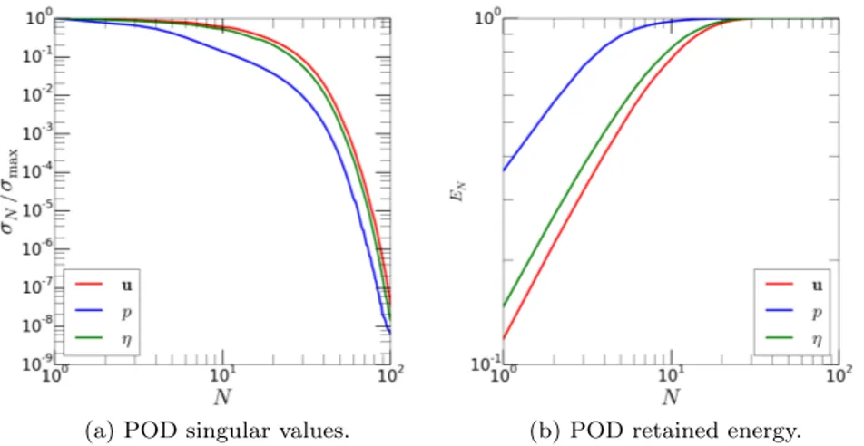
FSI ROM 1: Fig. 1 shows the POD singular values and retained energy as a function of the number N of POD modes for FSI ROM 1. It can be noticed that the decay of the singular values of fluid velocity and structure displacement is slower than the one of fluid pressure; moreover, the first POD mode of fluid pressure retains a larger energy (≈ 36%) than the first modes of structure displacement (≈ 15%) and fluid velocity (≈ 12%). Accordingly, the (relative) error analysis (Fig. 2a) shows that the reduced solution converges to the high-fidelity one, and that (except for small N ), the relative error on the pressure is smaller than the displacement one, which is smaller than
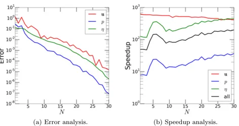
the velocity relative error. Employing only N = 30 POD modes out of the K = 1300 snapshots, velocity, displacement and pressure relative errors are of the order of 10−4, 10−5 and 10−7, respectively. Figure 2b shows that the overall speedup for large values of N is of at least two order of magnitudes. In particular, speedup for the explicit step is approximately constant for increasing N , while the speedup for the implicit steps is increasing for larger N since the number of required iterations for the implicit step decreases with N (see Fig. 7b and c for the maximum and average number of iterations, respectively).
(a) POD singular values. (b) POD retained energy.
Fig. 1 Results of the offline stage of FSI ROM 1: POD singular values and retained energy as a function of the number N of POD modes for fluid velocity, fluid pressure, and solid displacement.
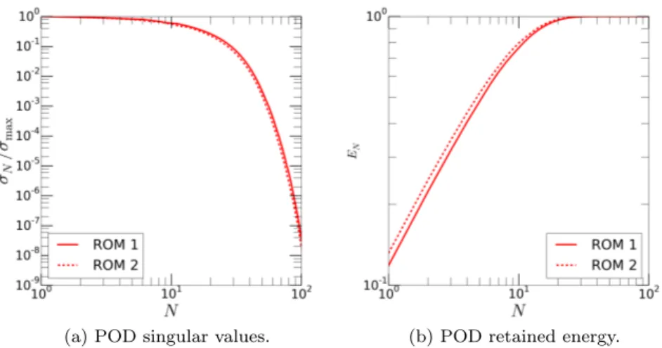
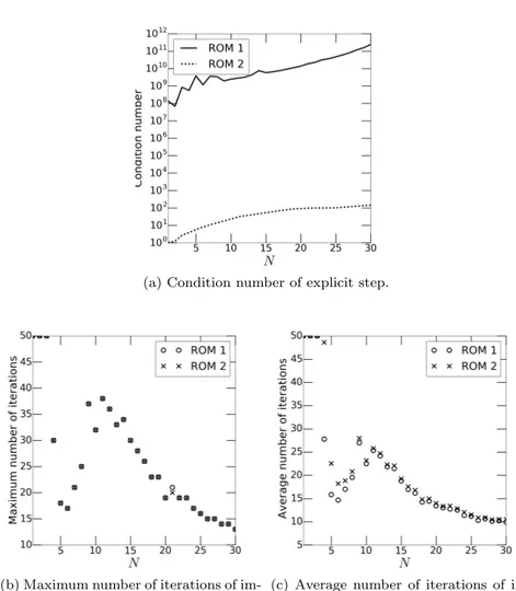
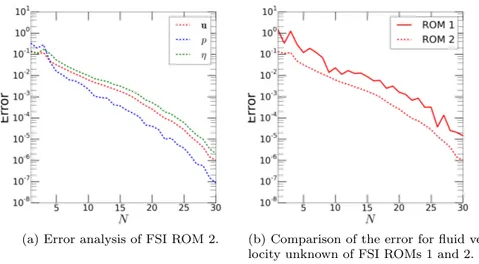
FSI ROM 2: Fig. 3 shows a comparison of the offline stage for ROMs 1 and 2. From Fig. 3b it can be noticed that, after the change of variable, the first auxiliary velocity z POD mode of FSI ROM 2 retains approximately 1.5% more energy than the first velocity u POD mode. The remaining variables are omitted since the pressure and displacement bases are the same as in FSI ROM 1. Moreover, Fig. 4a shows that the left-hand side matrix of the fluid viscous step 1(2)N (FSI ROM 2) is characterized by a condition number which is, for all N , at least 10 order of magnitude smaller than the one of 1(1)N (FSI ROM 1). The combination of these two remarks justifies the improvement in the error analysis for the velocity variables, shown in Fig. 5b. On average, the relative error on the velocity unknown obtained by FSI ROM 1 is seven times the one obtained by FSI ROM 2. Relative errors for the remaining unknowns are omitted because they are comparable among FSI ROMs 1 and 2. Moreover, we show in Fig. 6 the error analysis for the interface stress.
(a) Error analysis. (b) Speedup analysis.
Fig. 2 Error analysis and speedup analysis of FSI ROM 1, as a function of the number N of POD modes for fluid velocity, fluid pressure, and solid displacement.
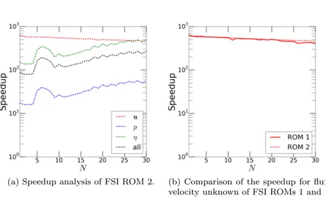
The plot clearly shows that FSI ROM 2 provides a better approximation of the interface stress for N > 20. Online performance (Fig. 7) are comparable to the ones obtained by FSI ROM 1. This is due to the fact that (i) the number of iterations to reach convergence in step 2(1)N and 2(2)N are the same as maximum values (Fig. 4b) and comparable on average (Fig. 4c), and (ii) the time to solve the explicit step does not depend strongly on N (Fig. 7b), even though step 1(2)N (FSI ROM 2) requires the solution of a linear system of size N × N (rather than 2N × 2N for step 1(1)N (FSI ROM 1)).
6 Conclusions and perspectives
Two semi-implicit reduced-order models for FSI problems have been proposed in this work, based on a POD–Galerkin approximation of an operator split-ting semi-implicit high-fidelity scheme. FSI ROM 1 is a standard Galerkin projection over the reduced spaces generated by POD. No supremizer enrich-ment is required, thanks to the operator splitting approach. Even though FSI ROM 1 shows good performance in terms of error analysis, its major draw-backs (when compared to FSI ROM 2) are related to the weak imposition of (9) by Lagrange multipliers. Numerical results of the previous section have shown that this is detrimental for several aspects of the ROM: increased sys-tem dimension of the fluid explicit step, increased condition number of the fluid explicit step, increased error for the velocity. FSI ROM 2, instead, stems from the idea that (9) can be easily imposed in a reduced-order framework by performing the change of variable (11). In this way, all the detrimental
(a) POD singular values. (b) POD retained energy.
Fig. 3 Comparison of the offline stage of FSI ROMs 1 and 2: POD singular values and retained energy as a function of the number N of POD modes for fluid velocity u (FSI ROM 1) and auxiliary fluid velocity z (FSI ROM 2).
effects of FSI ROM 1 are remedied. Moreover, better properties in terms of POD retained energy are also obtained. The combination of these two factors results in a better approximation of the fluid velocity. In particular, in FSI ROM 2, we try to separate in the fluid velocity the fluid-structure interaction component from the pure fluid part. Even though FSI ROM 1 suffers sev-eral drawbacks when compared to FSI ROM 2 (especially for what concerns the increased condition number), the approach proposed by FSI ROM 1 can be more easily integrated with existing reduced order modelling capabilities for fluid problems, since it does not require to change the existing computa-tions of fluid velocity basis funccomputa-tions. Nevertheless, especially for FSI ROM 1, a more detailed analysis of enrichment procedures shall be carried out to further investigate the stability of the resulting reduced problem, due to two saddle point structures to be taken into account (see Remarks 3 and 4). Future work will concern ROMs that are better able to face the hyperbolic nature of the problem. A more efficient separation at the reduced-order level of the parabolic and hyperbolic components of the system may decrease the number of basis functions required to obtain an accurate reduced description of the FSI problem.
Acknowledgements
We acknowledge the support by European Union Funding for Research and Innovation – Horizon 2020 Program – in the framework of European Research
(a) Condition number of explicit step.
(b) Maximum number of iterations of im-plicit step.
(c) Average number of iterations of im-plicit step.
Fig. 4 Comparison of the condition number of the left-hand side matrix of 1(1)N and 1(2)N (top) and of the maximum (bottom, left) and average (bottom, right) number of iterations required by 2(1)N and 2(2)N , as a function of the number N of POD modes for fluid velocity, fluid pressure, and solid displacement.
Council Executive Agency: H2020 ERC CoG 2015 AROMA-CFD project 681447 “Advanced Reduced Order Methods with Applications in Computa-tional Fluid Dynamics” and the PRIN project “Mathematical and numerical modelling of the cardiovascular system, and their clinical applications”. We also acknowledge the INDAM-GNCS project “Tecniche di riduzione della complessit`a computazionale per le scienze applicate” and INDAM-GNCS young researchers project “Numerical methods for model order reduction of PDEs”.
(a) Error analysis of FSI ROM 2. (b) Comparison of the error for fluid ve-locity unknown of FSI ROMs 1 and 2.
Fig. 5 Error analysis of FSI ROM 2, as a function of the number N of POD modes for fluid velocity, fluid pressure, and solid displacement.
Fig. 6 Error analysis of the interface stress for FSI ROMs 1 and 2, as a function of the number N of POD modes for fluid velocity, fluid pressure, and solid displacement.
References
1. Amsallem, D., Cortial, J., Farhat, C.: Towards real-time computational-fluid-dynamics-based aeroelastic computations using a database of reduced-order in-formation. AIAA Journal 48(9), 2029–2037 (2010)
2. Astorino, M., Chouly, F., Fern´andez, M.A.: Robin based semi-implicit coupling in fluid-structure interaction: Stability analysis and numerics. SIAM Journal on Scientific Computing 31(6), 4041–4065 (2010)
3. Badia, S., Nobile, F., Vergara, C.: Fluid–structure partitioned procedures based on Robin transmission conditions. Journal of Computational Physics 227(14),
(a) Speedup analysis of FSI ROM 2. (b) Comparison of the speedup for fluid velocity unknown of FSI ROMs 1 and 2.
Fig. 7 Speedup analysis of FSI ROM 2, as a function of the number N of POD modes for fluid velocity, fluid pressure, and solid displacement.
7027 – 7051 (2008)
4. Badia, S., Quaini, A., Quarteroni, A.: Splitting methods based on algebraic fac-torization for fluid-structure interaction. SIAM Journal on Scientific Computing 30(4), 1778–1805 (2008)
5. Ballarin, F., Manzoni, A., Quarteroni, A., Rozza, G.: Supremizer stabilization of POD–Galerkin approximation of parametrized steady incompressible Navier– Stokes equations. International Journal for Numerical Methods in Engineering 102(5), 1136–1161 (2015)
6. Ballarin, F., Rozza, G.: POD–Galerkin monolithic reduced order models for parametrized fluid-structure interaction problems. International Journal for Nu-merical Methods in Fluids 82(12), 1010–1034 (2016)
7. Ballarin, F., Sartori, A., Rozza, G.: RBniCS – reduced order modelling in fenics. http://mathlab.sissa.it/rbnics (2016)
8. Barrault, M., Maday, Y., Nguyen, N.C., Patera, A.T.: An ‘empirical interpolation’ method: application to efficient reduced-basis discretization of partial differential equations. Comptes Rendus Mathematique 339(9), 667–672 (2004)
9. Colciago, C.M.: Reduced order fluid-structure interaction models for haemody-namics applications. Ph.D. thesis, ´Ecole Polytechnique F´ed´erale de Lausanne, N. 6285 (2014)
10. Fern´andez, M.A.: Incremental displacement-correction schemes for incompress-ible fluid-structure interaction. Numerische Mathematik 123(1), 21–65 (2013) 11. Fern´andez, M.A., Gerbeau, J.F., Grandmont, C.: A projection semi-implicit
scheme for the coupling of an elastic structure with an incompressible fluid. In-ternational Journal for Numerical Methods in Engineering 69(4), 794–821 (2007) 12. Fern´andez, M.A., Landajuela, M., Mullaert, J., Vidrascu, M.: Domain Decompo-sition Methods in Science and Engineering XXII, chap. Robin-Neumann Schemes for Incompressible Fluid-Structure Interaction, pp. 65–76. Springer International Publishing (2016)
13. Fern´andez, M.A., Mullaert, J., Vidrascu, M.: Explicit Robin–Neumann schemes for the coupling of incompressible fluids with thin-walled structures. Computer Methods in Applied Mechanics and Engineering 267, 566–593 (2013)
14. Formaggia, L., Gerbeau, J., Nobile, F., Quarteroni, A.: On the coupling of 3D and 1D Navier–Stokes equations for flow problems in compliant vessels. Computer Methods in Applied Mechanics and Engineering 191(6–7), 561–582 (2001) 15. Guermond, J.L., Quartapelle, L.: On stability and convergence of projection
methods based on pressure poisson equation. International Journal for Numerical Methods in Fluids 26(9), 1039–1053 (1998)
16. Guidoboni, G., Glowinski, R., Cavallini, N., Canic, S.: Stable loosely-coupled-type algorithm for fluid–structure interaction in blood flow. Journal of Computational Physics 228(18), 6916–6937 (2009)
17. Hesthaven, J.S., Rozza, G., Stamm, B.: Certified Reduced Basis Methods for Parametrized Partial Differential Equations. SpringerBriefs in Mathematics. Springer International Publishing (2015)
18. Lassila, T., Manzoni, A., Quarteroni, A., Rozza, G.: A reduced computational and geometrical framework for inverse problems in hemodynamics. International Journal for Numerical Methods in Biomedical Engineering 29(7), 741–776 (2013) 19. Lassila, T., Quarteroni, A., Rozza, G.: A reduced basis model with parametric coupling for fluid-structure interaction problems. SIAM Journal on Scientific Computing 34(2), A1187–A1213 (2012)
20. Logg, A., Mardal, K.A., Wells, G.N.: Automated Solution of Differential Equa-tions by the Finite Element Method. Springer (2012)
21. Quarteroni, A., Formaggia, L.: Mathematical modelling and numerical simulation of the cardiovascular system. In: Computational Models for the Human Body, Handbook of Numerical Analysis, vol. 12, pp. 3–127. Elsevier (2004)
22. Quarteroni, A., Tuveri, M., Veneziani, A.: Computational vascular fluid dynamics: problems, models and methods. Computing and Visualization in Science 2(4), 163–197 (2000). DOI 10.1007/s007910050039. URL http://dx.doi.org/10.1007/s007910050039
23. Quarteroni, A., Valli, A.: Numerical approximation of partial differential equa-tions, vol. 23. Springer-Verlag Berlin Heidelberg (2008)
24. Rozza, G.: Reduced basis methods for Stokes equations in domains with non-affine parameter dependence. Computing and Visualization in Science 12(1), 23–35 (2009)
25. Rozza, G., Huynh, D.B.P., Manzoni, A.: Reduced basis approximation and a posteriori error estimation for stokes flows in parametrized geometries: roles of the inf-sup stability constants. Numerische Mathematik 125(1), 115–152 (2013) 26. Rozza, G., Huynh, D.B.P., Patera, A.T.: Reduced basis approximation and a posteriori error estimation for affinely parametrized elliptic coercive partial dif-ferential equations. Archives of Computational Methods in Engineering 15, 1–47 (2007)
27. Rozza, G., Veroy, K.: On the stability of the reduced basis method for Stokes equations in parametrized domains. Computer Methods in Applied Mechanics and Engineering 196(7), 1244–1260 (2007)