Quality of Experience and Adaptation Techniques for Multimedia Communications

(1)

(2)

(3)

Abstract

The widespread use of multimedia services on the World Wide Web and the advances in end-user portable devices have recently increased the user demands for better quality. Moreover, providing these services seamlessly and ubiquitously on wireless networks and with user mobility poses hard challenges. To meet these challenges and fulfill the end-user requirements, suitable strategies need to be adopted at both application level and network level. At the application level rate and quality have to be adapted to time-varying bandwidth limitations, whereas on the network side a mechanism for efficient use of the network resources has to be implemented, to provide a better end-user Quality of Experience (QoE) through better Quality of Service (QoS). The work in this thesis addresses these issues by first investigating multi-stream rate adaptation techniques for Scalable Video Coding (SVC) applications aimed at a fair provision of QoE to end-users. Rate Distortion (R-D) models for real-time and non real-time video streaming have been proposed and a rate adaptation technique is also developed to minimize with fairness the distortion of multiple videos with difference complexities. To provide resiliency against errors, the effect of Unequal Error protection (UXP) based on Reed Solomon (RS) encoding with erasure correction has been also included in the proposed R-D modelling. Moreover, to improve the support of QoE at the network level for multimedia applications sensitive to delays, jitters and packet drops, a technique to prioritise different traffic flows using specific QoS classes within an intermediate DiffServ network integrated with a WiMAX access system is investigated. Simulations were performed to test the network under different congestion scenarios.

(4)

(5)

Acknowledgements

First and above all, I praise God, the almighty for providing me this opportunity and grant-ing me the capability to proceed successfully. This thesis appears in its current form due to the assistance and guidance and prayers of several people. I would therefore like to offer my sincere thanks to all of them.

I am thankful to my adviser Velio Tralli for his support, guidance and ideas that he gave during my Ph.D which made this thesis possible. I appreciate all his contributions of time and ideas to make my Ph.D experience productive and stimulating. The joy and enthusiasm he has for his research was contagious and motivational for me, even during tough times in the Ph.D pursuit. I am grateful to Gianluca Mazzini and Andrea Conti for their active support whenever I needed.

I am also thankful to Maria Martini for her supervision, guidance and funding me in

Royal Society Project for the months that I spent for my research in Kingston University,

London.

I cannot forget the forever and everlasting support of my parents and siblings. I am thankful to my elder brother Asif for his financial support before starting my Ph.D and my parents and siblings for theirs prayers. In short I cannot express my gratitude to them in words.

I am thankful to my colleagues in TLC lab. They were always helpful and cooperative to me in academic and non academic acttivites, to name few in particular are Danilo, Honorine and Sergio.

(6)

My time in Ferrara is the best I had so far and it was made enjoyable in large part due to the many friends and groups that became a part of my life. In particular I am thankful to all my friends of residential college “Cenacolo” where I found myself as to be in my home. I will also extend my gratitude to Lena Fabbri as she helped me a lot, for official work both in and out of university and during my stay in Ferrara.

Last but not the least I am thankful to University of Ferrara for giving me the opportu-nity and funding me during these three years of my Ph.D.

Abdul Haseeb

University of Ferrara, Italy

March 2012

(7)

DEDICATION

To my Loving Parents

!

and

"!

(8)

List of Tables

3.1 Comparison between the two semi-analytical model in (3.9) and (3.10) with respect to the minimum and maximum RMSE and the coefficient of determina-tion R2 evaluated for each GOP (GOP size equal to 16) of five video sequence with CIF resolution and frame rate of 30 fps. The video are encoded with one base layer (QP equal to 38) and two enhancement layers (QP equal to 32 and 26), both with 5 MGS layers and a weights vector equal to [3 2 4 2 5]. . . 26

(11)

3.2 Average MSE of each video sequence with equal-rate (ER) assignment and rate adaptation with the proposed algorithm (OPT). Total bandwidth is equal to 3000 kbps. . . 34 3.3 Average modified MSE difference ∆av, average MSE difference δav and MSE

variance in each GOP interval. Comparison between the proposed algorithm (OPT) and equal-rate (ER) assignment with bandwidth equal to 3000 kbps. . . 36 4.1 Percentage of the overhead and expected distortion dGQ,loss in term of MSE

with respect to the full quality video streams (Q= 10 and G = 8), for different values of RTP packet error probability andα parameter in the EEP profile. . . . 51 4.2 Average received distortion,D∗_rec_,av, expected distortion, D∗_av, and encoding

dis-tortion, D∗_enc_,av, in term of the MSE for different video sequences, GOP size G, and packet-erasure rate values Pe,rt p, resulting from the proposed rate-adaptation

algorithm. Available bandwidth is Rc=7000 kbps. . . 53

5.1 Average MSE over 26 GOPs obtained with the model (5.1) and proposed model in the transmission of the training set of 6 videos. . . 67 5.2 Average MSE over 26 GOPs obtained with the model (5.1) and proposed model

in the transmission of 4 videos not included in the training set. . . 67 6.1 WiMAX and DiffServ traffic class mapping . . . 78

List of Figures

2.1 Principle of encoding. . . 7

(12)

2.2 Principle of decoding. . . 7 2.3 Multi-layer structure with additional inter-layer prediction for enabling spatial

scalable coding. . . 9 2.4 Enhancement temporal (a) and quality (b) layer prediction for a GOP of 8 frames. 10 2.5 Fine granular scalability. . . 13 3.1 R-D Model (straight line), according to eq. (3.10) fitting the empirical R-D

relationship for the GOP with the worst RMSE with reference to Table 3.1. . . 26 3.2 Rate assigned by our adaptation algorithm in each GOP, with bandwidth equal

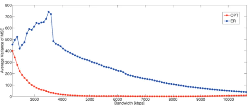
to 3000 kbps. . . 36 3.3 Variance of the MSE averaged over 15 GOPs, with different bandwidth

val-ues. Comparison between the proposed algorithm (OPT) and equal-rate (ER) assignment. . . 37 3.4 Average number of iterations required by our adaptation algorithm (OPT) and

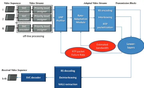
golden search algorithm (GSA) to converge. . . 37 4.1 System architecture. Each sequence is encoded to fully support temporal and

quality scalability and a priority level is assigned to the NALUs. The UXP pro-filer evaluates the overhead required according to a certain protection policy and RTP packet failure rate, and provides R-D information to the Adaptation module. The Adaptation module extracts sub-streams according to the esti-mated bandwidth and sends the data bytes to the RS encoder. The resulting codewords are then encapsulated in a transmission block, interleaved in RTP packets and forwarded to the lower layers. The receiver performs the inverse operations (RS decoding and deinterleaving) in order to extract the NALUs which are sent to the SVC decoder. . . 42

(13)

4.2 Transmission Sub-Block (TSB) structure. Following the priority level, the NALUs of one GOP are placed into one TSB according to a given UXP profile (protec-tion class) from upper left to lower right. The columns of one ore more TSB

are then encapsulated into RTP packets . . . 45

4.3 Resulting logarithmic FEP for the first I frame of Football (byte size equal to 11519) mapped to RS codewords (128,m) at different RTP packet error proba-bility. . . 48

4.4 R-D Model (straight line), according to eq. (3.10) fitting the empirical R-D relationship for one GOP (size G equal to 8) of the Football test-sequence with different error probabilities andα=30. The lower curve refers to the R-D relationship of the encoder. . . 50

5.1 Proposed model forα with R2_{= 0.987 and RMSE = 1598 . . . 61}

5.2 Proposed model forβ with R2= 0.973 and RMSE = 21.2 . . . 62

5.3 Proposed model for (BL) with R2= 0.979 and RMSE = 22.98 . . . 62

5.4 Proposed model for (EL) with R2= 0.985 and RMSE = 79.36 . . . 63

5.5 R-D comparison among model in eq (5.1), proposed model and actual values for two sample GOPs. . . 64

5.6 BL and EL rates over 26 GOPs for two sequences in the training set (Football and City) and two sequences outside the training set (Mobile and Foreman). The marker points refer to the original BL and EL rates, whereas the solid lines refer to rates estimated from (5.4) and (5.5), respectively. . . 65

5.7 Averaged MSE for each GOP of two sample videos in the transmission over bandwidth constrained channel with rate adaptation. Figures Football and City refer to the transmission of the 6 videos of the training set (Rc= 3500 kbps), wheres figures Mobile and Foreman refer to the transmission of 4 videos not included in the training set (Rc= 3000 kbps). . . 68

(14)

6.1 DiffServ Code Point field. . . 74

6.2 IEEE 802.16 QoS Architecture . . . 76

6.3 WiMAX and DiffServ Network Simulation Scenario . . . 77

6.4 Priority Queuing Implemented in Edge Router . . . 79

6.5 Packets dropped without DiffServ support. . . 80

6.6 Delay without DiffServ support and with 100% load. . . 81

6.7 Delay with DiffServ support and 100% load. . . 81

6.9 Delay with DiffServ support and 112.5% load . . . 82

6.8 Delay without DiffServ support and 112.5% load. . . 82

6.10 Delay without DiffServ support and 125% load . . . 83

6.11 Delay with DiffServ support and 125% load . . . 83

6.12 VoIP service jitters in networks with and without DiffServ. . . 84

(15)

Chapter 1 Introduction

The popularity of multimedia applications is rapidly increasing. Multimedia applications include video on demand, IP-TV, sport broadcasting, VoIP as well as real-time streaming. They have become reality now thanks to the achievements in the compression and storage technologies and the advances in transmission systems. The penetration of end user devices such as 3G mobile devices, portable multimedia players (PMP), HDTV flat-panel displays, and the availability of wired and wireless broadband internet access provides different ways to deliver these multimedia services. Nevertheless, in such environment providing contents everywhere while achieving efficiency is a challenge. Scalable Video Coding (SVC) which is the extension of Advance Video Coding standard H.264/AVC provides an attractive solu-tion to support video transmission in modern communicasolu-tion systems. In SVC some parts of the encoded video can be removed so that the video stream can be adapted to the network conditions. Moreover, SVC can fulfill the requirements of the users with different termi-nal capabilities and varying network conditions by providing spatial, temporal and quality scalabilities. Multimedia contents like voice and video can tolerate only to some extent jit-ters, delays and packet drops but they need sufficiently wide bandwidth. WiMAX, which is considered an alternative to DSL, can provide wireless broadband connectivity with its rich set of QoS classes for different types of multimedia applications which can be further

(16)

2 CHAPTER 1. INTRODUCTION

translated to the intermediate wired networks like DiffServ.

1.1 Scope of the Thesis

The aim of this thesis was to study the issues related to the provision of better Quality of Experience (QoE) for multimedia applications like video and voice and in this context particular emphasis was given to Scalable Video Coding (SVC). This thesis proposes new continuous Rate-Distortion (R-D) models both for real-time and non real-time videos. New rate adaptation techniques based on fairness for multi-stream video communication are also developed and applied to both the real and non real-time R-D models. Moreover, to further enhance the model an Unequal Error Protection (UXP) mechanism is introduced to cope with errors during transmission. The non real-time R-D model takes advantage of the SVC encoder to get the original R-D points from the video sequence and find the best possible R-D couple by curve fitting technique. To develop R-D models for real-time video transmis-sion, raw video sequences are exploited to get Spatial Indexes (SI) and Temporal Indexes (TI), which are also referred as spatial and temporal complexities, to be used to predict the parameters of the R-D model, as well as the rate prior to the encoding process of the videos. The multimedia information may flow through several networks before reaching to the final destination. This can be the cause of quality degradation for the application in use because of the bandwidth limitation of heterogeneous networks, the absence of prioritizing policies for delay sensitive traffic in intermediate networks, and network congestion, just to name few of them. To address this issue in limited context a solution for WiMAX and DiffServ interworking is provided in which VoIP traffic from WiMAX network entering DiffServ network is prioritized to get a preferential treatment in DiffServ networks and minimize delays, jitters and packets drops.

(17)

1.2. OUTLINE OF THESIS 3

1.2 Outline of Thesis

This thesis is organized as follows: In Chapter 2 the basic concepts of SVC are explained. In Chapter 3 a semi-analytical R-D model is proposed for non real-time SVC and, also a multi-stream rate adaptation technique based on fairness among videos is developed. The rate adaptation technique is then applied to the proposed R-D model and compared the results with the Equal Rate (ER) scheme. In Chapter 4, the proposed R-D model and rate adaptation technique of Chapter 3 is investigated for error prone channels using Unequal Error Protection (UXP). The UXP is based on Reed-Solomon (RS) encoding with erasure correction. In Chapter 5 a R-D model for SVC real-time video streams is proposed. The proposed model exploits SI and TI values GOP by GOP from the raw videos. The SI and TI values are then used to predict the rate of the video before encoding. The Proposed model is then used for multi-stream video delivery using the rate adaptation technique adopted in Chapter 3. The results of the proposed R-D model are compared with those obtained with R-D model in Chapter 3 by applying the rate adaptation technique. In Chapter 6 the interworking of the WiMAX and DiffServ heterogeneous network is described. In this proposed research work the Unsolicited Grant Service (UGS) from WiMAX network is mapped to the Expedited Forwarding (EF) service of DiffServ network. Priority Queuing (PQ) is applied inside the EF to deliver the delay sensitive traffic i.e. VoIP. The network is then tested on several congested scenario to test its efficiency to delays, jitters and packets drops with and without DiffServ network.

A part of work included in this thesis is published in [30] [46] [47] and [48] during my PhD.

(18)

(19)

Chapter 2 Overview of Scalable Video Coding

2.1 Introduction

Advances in video coding techniques and standardization along with the rapid development and improvements of network infrastructures, storage capacity and computing powers are enabling an increasing number of video applications. Applications area, today, range from MMS, video telephony and video conferencing over mobile TV etc. For these applications, a variety of video transmission and storage systems may be employed.

Due to the rapidly growing number of portable and non-portable devices, there is a strong need of a video standard that can be scaled according to the user and network needs. Because of all theses consideration, scalability and flexibility are key points for the near future of video services, whether these are new services or evolution of existing services. Such scalability is need not only on the architecture and infrastructure levels, but also at the content level [1].

Scalable Video Coding provides the appropriate tools to efficiently implement content scalability and portability. It is the latest scalable video-coding solution, and has been stan-dardized recently as an amendment to the now well-known and widespread H.264/AVC standard [2] by the Joint Video Team (JVT).

(20)

6 CHAPTER 2. OVERVIEW OF SCALABLE VIDEO CODING

In general, a video bit stream is called scalable when parts of the stream can be re-moved in a way that the resulting substream forms another valid bit stream for some target decoder, and the substream represents the source content with a reconstruction quality that is less than that of the complete original bit stream but is high when considering the lower quantity of remaining data. Bit streams that do not provide this property are referred to as single-layer bit streams [1]. Another benefit of SVC is that a scalable bit stream usually contains parts with different importance in terms of decoded video quality. This property in conjunction with unequal error protection is especially useful in any transmission scenario with unpredictable throughput variations and/or relatively high packet loss rates. By us-ing a stronger protection of the more important information, error resilience with graceful degradation can be achieved up to a certain degree of transmission errors.

2.2 Concept of H.264/AVC Extension to H.264/SVC

In SVC encoding is performed once while it can be decoded multiple times to get the re-quired bit stream as shown in figure 2.1. It states that the encoder has to encode once the bit stream which has details about spatial temporal and quality scalabilities. This scalable stream is then sent to the user and the user decode the stream according to its own require-ment.

The principle of decoding is show in figure 2.2. As in Advance Video Coding, the en-coding of the input video is performed at the Macro block basis. As the codec is based on the layer approach to enable spatial scalability, the encoder provides a down sampling filter stages that generates the lower resolution signal for each spatial layer. Encoder algorithm (not mention here in this thesis) may select between inter and intra coding for block shaped regions of each picture. 12 The video sequence is temporally decomposed into texture and motion information. Motion information from the lower layer may be used for prediction of the higher layer. The application of this prediction is switchable on a macro block or

(21)

2.2. CONCEPT OF H.264/AVC EXTENSION TO H.264/SVC 7

Figure 2.1: Principle of encoding.

Figure 2.2: Principle of decoding.

block basis. In case of intra coding, a prediction from surrounding macro blocks or from co-located macro blocks of other layers is possible. These prediction techniques do not employ motion information and hence, are referred to as intra prediction techniques. Fur-thermore, residual data from lower layers can be employed for an efficient coding of the current layer. The redundancy between different layers is exploited by additional inter-layer prediction concepts that include prediction mechanisms for motion parameters as well as for texture data (intra and residual data).The residual signal resulting from intra or mo-tion compensated inter predicmo-tion is transform coded using AVC features. Three kinds of prediction applied here are –Inter layer motion prediction, inter layer residual prediction

(22)

and Inter layer intra prediction. An important feature of the SVC design is that scalability is provided at a bit-stream level. Bit-streams for a reduced spatial and/or temporal resolu-tion are simply obtained by discarding NAL units (or network packets) from a global SVC bit-stream that are not required for decoding the target resolution. NAL units of PR slices can additionally be truncated in order to further reduce the bit-rate and the associated re-construction quality. Thus, one of the main design goals was that SVC should represent a straightforward extension of H.264/AVC. As much as possible, components of H.264/AVC are re-used, and new tools are only be added for efficiently supporting the required types of scalability. As for any other video coding standard, coding efficiency has always to be seen in connection with complexity in the design process.

2.3 Types of Scalabilities

Three scalability methods are possible in SVC, named temporal, spatial and SNR scalabil-ity, that allow to extract a sub-stream in order to meet a particular frame rate, resolution and quality, respectively. Each picture of a video sequence is coded and encapsulated into sev-eral Network Abstraction Layer Units (NALUs), which are packets with an integer number of bytes. Three key ID values, i.e. dependency id, temporal id, and quality id, are embed-ded in the header by means of the high level syntax elements, in order to identify spatial, temporal and quality layers.

2.3.1 Spatial scalability

For supporting spatial scalable coding, SVC follows the conventional approach of multiple-layer coding, which is also used in MPEG-2 Video / H.262, H.263, and MPEG-4 Visual. Each layer corresponds to a supported spatial resolution and is identified by a layer or de-pendency identifier D. The layer identifier D for the spatial base layer is equal to 0, and it is

(23)

2.3. TYPES OF SCALABILITIES 9

Figure 2.3: Multi-layer structure with additional inter-layer prediction for enabling spatial scalable coding.

increased by 1 from one spatial layer to the next. In each layer, motion-compensated pre-diction and intra coding are employed as for single-layer coding. But in order to improve the coding efficiency in comparison to simulating different spatial resolutions, additional inter-layer prediction mechanisms are incorporated.. Although the basic concept for sup-porting spatial scalable coding is similar to that in prior video standards, SVC contains new tools that simultaneously improve the coding efficiency and reduced the decoder complex-ity overhead in relation to single-layer coding. In order to limit the memory requirements and decoder complexity, SVC requires that the coding order in base and enhancement layer is identical. All representations with different spatial resolutions for a time instant form an access unit and have to be transmitted successively in increasing order of their layer iden-tifiers D. But lower layer pictures do not need to be present in all access units, which make it possible to combine temporal and spatial scalability as illustrated in Figure 2.6.

2.3.2 Temporal scalability

Temporal scalability can be achieved by means of the concept of hierarchical predic-tion. Each picture in one GOP is identified by a hierarchical temporal index or level t ∈ {0, 1, . . . , T }. The encoding/decoding process starts from the frame with the temporal in-dex t = 0 that identifies a key-picture which must be intra-coded (I frame), in order to allow a GOP-based decoding. The remaining frames of one GOP are typically coded as

(24)

(a)

(b)

Figure 2.4: Enhancement temporal (a) and quality (b) layer prediction for a GOP of 8 frames.

P/B-pictures and predicted according to the hierarchical temporal index, thereby allowing to extract a particular frame rate. An implicit encoding/Decoding Order Number (DON) can be set up according to the temporal index and frame number of each frame.

In Figure 2.4(a) we show an example of the hierarchical prediction structure for a GOP with 8 pictures. The DON is obtained by ordering the pictures according to the temporal

(25)

index. If more than one frame have the same temporal level, the DON is assigned according to the picture index. Let us note that the last frame is encoded as P-frame in order to allow a GOP-based decoding, as mentioned before.

2.3.3 SNR scalability/Quality scalability

The SNR scalability allows to increase the quality of the video stream by introducing re-finement layers. Two different possibilities are now available in SVC standard and imple-mented in the reference software [3], namely Coarse Grain Scalability (CGS) and Medium Grain Scalability (MGS). CGS can be achieved by coding quality refinements of a layer using a spatial ratio equal to 1 and inter-layer prediction. However, CGS scalability can only provide a small discrete set of extractable points equal to the number of coded layers. Here the focus is on MGS scalability which provides finer granularity with respect to CGS coding by dividing a quality enhancement layer into up to 16 MGS layers. MGS coding distributes the transform coefficients obtained from a macro-block by dividing them into multiple sets. The R-D relationship and its granularity depends on the number of MGS layers and the coefficient distribution, [4]. In [4] the authors analyzed the impact on perfor-mance of different numbers of MGS layers with different configurations used to distribute the transform coefficients. We also verified their results, by noting that more than five MGS layers reduce the R-D performance without giving a substantial increase in granularity. This is mainly due to the fragmentation overhead that increases with the number of MGS layers. While extracting an MGS stream two possibilities are available in the reference soft-ware: a flat-quality extraction scheme, and a priority-based extraction scheme. The second scheme requires a post-encoding process, executed by an entity denoted as Priority Level Assigner, that computes a priority level for each NALU. It achieves higher granularity, as well as better R-D-performance [5]. The priority level ranges from 0 to 63, where 63 is in-tended for the base-layer, and is assigned to each NALU according to quality dependencies

(26)

and R-D improvement. Nevertheless, in order to exploit the temporal scalability at the de-coder side, we re-assign different priority levels to the base-layer frames (those with q= 0), according to their temporal indexes, as specified afterwards. This feature is only exploited by the UXP profiler in subsection 4.2.2 and therefore does not change the 6-bit header of the packet which is necessary to perform the quality-based extraction. The R-D performance of the quality layers can be improved by using quality frames for motion compensation and introducing the concept of key-picture, which allows for a trade-off between drifting and coding efficiency. Nevertheless, this tool should not be applied in a rate-adaptation framework where all quality layers are often discarded by the rate adaptation module as exemplified in Figure 2.3(b).

2.3.3.1 Coarse Grain Scalability (CGS)

Coarse grain scalability (CGS) can be viewed as a special case of spatial scalability in H.264 SVC, in that similar encoding mechanisms are employed but the spatial resolution is kept constant. More specifically, similar to spatial scalability, CGS employs inter-layer prediction mechanisms, such as prediction of macroblock modes and associated motion parameters and prediction of the residue signal [1]. CGS differs from spatial scalability in that the up-sampling operations are not performed. In CGS, the residual texture signal in the enhancement layer is re-quantized with a quantization step size that is smaller than the quantization step size of the preceding CGS layer. SVC supports up to eight CGS layers, corresponding to eight quality extraction points [6], i.e., one base layer and up to seven enhancement layers.

2.3.3.2 Medium Grain Scalability (MGS)

While CGS provides quality scalability by dropping complete enhancement layers, MGS provides a finer granularity level of quality scalability by partitioning a given enhancement

(27)

layer into several MGS layers [1]. Individual MGS layers can then be dropped for quality (and bit rate) adaptation.

a) Splitting Transform Coefficients into MGS Layers:Medium grain scalability (MGS)

splits a given enhancement layer of a given video frame into up to 16 MGS layers (also referred to as quality layers). In particular, MGS divides the transform coefficients, ob-tained through transform coding of a given macroblock, into multiple groups. Each group is assigned to a prescribed MGS layer.

b) Bit Rate Extraction:With MGS encoding, the video bit rate is adjusted by dropping

enhancement layer NALUs, one at a time, until the target bit rate is achieved. No NALUs are dropped from the base layer.

2.3.3.3 Fine Grain Scalability (FGS)

In order to support fine-granular SNR scalability, so-called progressive refinement (PR) slices have been introduced. Each PR slice represents a refinement of the residual signal that corresponds to a bisection of the quantization step size (QP increase of 6). These signals are represented in a way that only a single inverse transform has to be performed for each transform block at the decoder side. The ordering of transform coefficient levels in PR slices allows the corresponding PR NAL units to be truncated at any arbitrary byte-aligned point, so that the quality of the SNR base layer can be refined in a fine-granular way. Figure 2.5 shows general concepts of Fine Granular Scalability in terms of layers.

(28)

The main reason for the low performance of the FGS in MPEG-4 is that the motion compensated prediction (MCP) is always done in the SNR base layer. In the SVC design, the highest quality reference available is employed for the MCP of non-key pictures as depicted in Figure 2.5. Note that this difference significantly improves the coding efficiency without increasing the complexity when hierarchical prediction structures are used. The MCP for key pictures is done by only using the base layer representation of the reference pictures. Thus, the key pictures serve as resynchronization points, and the drift between encoder and decoder reconstruction is efficiently limited. In order to improve the FGS coding efficiency, especially for low-delay IPPP coding, leaky prediction concepts for the motion-compensated prediction of key pictures have been additionally incorporated in the SVC design.

2.4 Backward Compatibility

It is desirable in SVC scheme that a so called base layer be compatible with non Scalable video coding standards like AVC. It is also desired that additional scalable layers should be carried out in such a way that non-scalable video decoders, which have no knowledge of scalability, will ignore all scalable layers and only decode the base layer [7]. For these coded data that follow H.264/AVC and to ensure compatibility with existing H.264/AVC decoder, another new type of NAL (type 20) is used. This NAL carry the header informa-tion [8]. The base layer by design is compatible to H.264/AVC. During transmission, the associated prefix NAL units, which are introduced by SVC and when present are ignored by H.264/AVC decoders, may be encapsulated within the same RTP packet as the H.264/AVC VCL NAL units, or in a different RTP packet stream(when Multi session transmission mode is used) [9].

When using Multi session transmission mode-When a H.264/AVC compatible subset of the SVC base layer is transmitted in its own session in multi session transmission mode,

(29)

2.4. BACKWARD COMPATIBILITY 15

the packetization of RFC 3984 must be used, such that RFC 3984 of receivers can be part of multi transmission mode and receive only this session [10]. When using Single session transmission mode-When an H.264/AVC compatible subset of SVC base layer is transmitted using single session transmission, the packetization of RFC 3984 must be used, thus ensuring compatibility with RFC 3984 receivers [8].

(30)

(31)

Chapter 3 Rate Adaptation Using MGS for SVC

3.1 Introduction

H.264 Advanced Video coding (AVC) standard with scalable extension, also called Scal-able Video Coding (SVC) [1], provides flexibility in rate adaptation by coding an origi-nal video sequence into a scalable stream. Three scalability methods are possible in SVC, named temporal, spatial and SNR scalability, that allow to extract a sub-stream in order to meet a particular frame rate, resolution and quality, respectively. Due to the dierent com-plexities of the scenes composing a video sequence, the relationships between the rate and the quality of a set of videos can be really different among them. If individual video streams are transmitted to different users in a broadcast dedicated channel, as for instance in the case of on-demand IP-TV services [11], an equal rate allocation can lead to unacceptable distor-tion of high-complexity videos with respect to low-complexity ones. Adaptive transmission strategies must be investigated to dynamically optimize the quality of experience (QoE) of each end-user.

In this chapter, we focus on rate adaptation, also called in literature statistical multi-plexing, of SNR-scalable video streams, with a fixed temporal and spatial resolution. Many

(32)

18 CHAPTER 3. RATE ADAPTATION USING MGS FOR SVC

contributions exist in the literature that provide rate adaptation exploiting the Fine Gran-ularity Scalability (FGS) tool, e.g. [12],[13] and [14]. FGS coding allows to extract an arbitrary rate-distortion (R-D) point while maintaining the monotonic non-decreasing be-havior of the R-D curves. Nevertheless FGS mode has been removed from SVC, due to its complexity.

Two different possibilities for the SNR scalability tool are now available in SVC stan-dard and implemented in the reference software [3], namely Coarse Grain Scalability (CGS) and Medium Grain Scalability (MGS). CGS can be achieved by coding quality refinements of a layer using a spatial ratio equal to 1 and inter-layer prediction. However, CGS scalabil-ity can only provide a small discrete set of extractable points equal to the number of coded layers. MGS provides a ner granularity of quality scalability by dividing a CGS layer into up to 16 MGS layers. The granularity can be also improved if a post-processing quality layer (QL) insertion and a consequent quality-based extraction is performed with the aim to optimize the R-D performance [5]. With this tool MGS can be seen as alternative to the FGS coding.

The rest aim of this work is to analyze the performance of the MGS with QL and to provide a general R-D model. Other contributions exist in literature that estimate the R-D model for SNR-based scalable stream, with CGS and MGS, e.g. [15], [16], either analytical and semi-analytical. The analytical models are dependent on the probability distribution of discrete cosine transform (DCT) coefficients and often incur in a loss of accuracy. To achieve higher accuracy, semi-analytical R-D models are preferable. The semi-analytical models are based on parametrized functions that follow the shape of analytically derived functions, but are evaluated through curve-fitting from a subset of the rate-distortion em-pirical data points. In [16], the authors proposed an accurate semi-analytical square-root model for MGS coding and compared it with linear and semi-linear model. They concluded that the best performance is obtained by changing the model according to a parameter that

(33)

3.1. INTRODUCTION 19

estimates the temporal complexity, evaluated before encoding the entire sequence. How-ever, a general model, that is able to estimate the R-D relationship of a large range of video sequences, is necessary to perform analytical optimization of the rate-adaptation problem. Besides, they did not consider the post-processing QL insertion that produces a variation of the R-D performance.

In [17] the authors proposed a general semi-analytical rate-distortion model for video compression, also verified in [18] for SVC FGS layer, where the rate and the distortion have an inverse relationship. Three sequence-dependent parameters must be estimated through the knowledge of six empirical R-D points. We have also verified this model with reference to SNR scalability with MGS and QL. The high accuracy of the results led us to investi-gate a simplified model with lower complexity, where the number of R-D points can be reduced by eliminating one of the parameters to estimate. Thus, we propose and compare a simplified two-parameters semi-analytical rate-distortion model. This simplification has two main advantages: (i) only four empirical points are needed by the curve fitting algo-rithm to achieve good performance, (ii) it allows the derivation of a low-complexity optimal procedure to solve the multi-stream rate-adaptation problem, with a maximum number of iterations equal to the number of streams involved in the optimization.

This Chapter has the following main contributions: in section 3.2, a general optimiza-tion problem is formulated with the aim to provide the maximum quality to each video while minimizing their distortion difference, and by fulfilling the available bandwidth. In section 3.3 we analyze and verify two similar semi-analytical models for MGS with QL by comparing them with respect to complexity and the normally used goodness parame-ters: the root mean square error (RMSE) and the coefficient of determination R2 [19]. An optimum and computationally efficient procedure to solve the relaxed general problem is derived in section 3.4, with a discussion about complexity and optimality. Finally the nu-merical results, discussed in section 3.5, show (i) the goodness of our framework by looking at the error between the relaxed and discrete solutions, (ii) the performance improvement

(34)

with respect to a blind adaptation, and (iii) the complexity of the proposed algorithm with respect to a sub-optimal golden search algorithm proposed in literature.

3.2 General Problem Formulation for Multi-Stream Rate

Adaptation

In general, the aim of multi-stream rate adaptation is to optimize a certain number of utility functions Uiwith respect to a quality metric and according to rate constraints [20]. Before

or after the encoding process the original high quality video must be adapted, to meet a particular QoE metric depending on spatial, temporal and SNR resolutions.

In this section we provide a general problem formulation for multi-stream rate adap-tation. Let K be the number of streams involved in the optimization. Given a set of lossy compression techniques 1, ..., Nk, we can define in general Dk = d1,k, ..., dN,k, k= 1, ..., K

as the set of distortion values for the k-th stream. Let us note that its cardinality|Dk| = Nk

is generally not equal for each video source, as in the case of high- flexibility SNR-based compression techniques.

The rate-distortion theory evaluates the minimum bit-rate Rk required to transmit the k-th stream with a given distortion d_n_,k, by defining a functionF_k that maps the distortion to the rate, i.e.

Fk: dn,k→ R+

d_n_,k → Rk= Fk(dn,k) (3.1)

(35)

3.2. GENERAL PROBLEM FORMULATION FOR MULTI-STREAM RATE

ADAPTATION 21

F_k_(d_i_,k_{) > F}_k_(d_j_,k_), _d_i_,k_{, d}_j_,k_{: d}_i_,k_{< d}_j_,k _(3.2) When multiple streams have to be transmitted in a shared channel the rate adaptation algorithm must choose at each time slot and according to one optimization strategy, the best vector D∗= [D1, ..., D∗_K] ∈ D = D1× ... × DK.D contains all the possible combinations of

the elements of Dk, k= 1, ..., K and has cardinality N = ∏K_k₌₁Nk.

The main purpose of multi-stream rate adaptation is to provide the minimum distor-tion, or equivalently the maximum rate according to assumption (2), to each video under a total bit-rate constraints Rc. However, the solution of such problem can generally lead to

large distortion variations among different streams, due to the different complexity of video sources. Quality fairness is an important issue that must be addressed when multiple videos from different sources are transmitted in a shared channel. In [13] the authors have shown that, given a continuous decreasing exponential R-D relationship with a constant exponent equal for each source, the solution to the problem of minimizing the distortion variations is also the solution to the problem of minimizing the total average distortion. However, an exponential R-D relationship is not an accurate model for all the different video com-pression techniques, particularly for the SVC SNR scalable stream [13]. Thus, a general multi-objective problem has to be formulated and a continuous relaxation of the problem leads to some particular simplification under certain assumptions. The general objective of our proposed framework is to minimize the differences among the distortions provided to each video stream while maximizing the sum of the rates until a maximum bit-rate is met. As mentioned above, these two objectives alone can generally lead to different solutions.

Thus, we formulate the general problem as a multi-objective problem:

min

(36)

22 CHAPTER 3. RATE ADAPTATION USING MGS FOR SVC max DDD∈D K

∑

k=1 F_k_(D_k₎ (3.4) s.t. K

∑

k=1 F_k_(D_k_{) ≤ R}_c _(3.5) where ∆(Di, Dj) =      0 if (i,j)_{∈ X}D∨(j, i) ∈ XD |Di− Dj| otherwise (3.6) with

XD = {(i, j) ∈ Z2:(Di= Dmax,i∧ Dj> Di) ∨ (Di= Dmin,i∧ Dj< Di)} (3.7)

and Dmin,i = minndn,i, Dmax,i = maxndn,i. The operators ∧ and ∨ are the logic ”AND”

and ”OR”, respectively.

Ideal fairness among the distortion values assigned to the multiple video streams, i.e.

Di= Dj, ∀i 6= j, is hard to be achieved. This fact is due to (i) the discretization of the R-D

relationship and (ii) the presence of the minimum and the maximum distortion values for each source that are related to the complexity of each video and which can be very differ-ent. The definition of the fairness metric takes this fact into account. In fact, the difference among video distortions ∆(Di, Dj) is slightly modified to take into account the minimum

and the maximum constraints. It is worth noting that, under the assumption (3.2), this prob-lem admits a feasible solution only if at least the sum of the minimum rates of the video sequences is supported by the transmission bandwidth Rc, i.e

K

∑

k=1

(37)

3.3. RATE DISTORTION MODEL FOR MGS WITH QUALITY LAYER 23

otherwise a certain number of videos are not admitted in the transmission until this constraint is not satisfied. The solution of the problem in (3.3)-(3.5) requires in general an exhaustive search in the space D of all possible vectors. If N becomes large the required complexity can be not suitable for real-time adaptation. On the other hand if N is small, i.e there are few video sources as well as few related R-D points, the problem solution can lead to a waste of the available bandwidth and a large distortion differences among multiple videos.

In the next section we will propose a semi-analytical R-D model with reference to the SNR scalability tool of SVC with MGS and QL layers [5]. This continuous model will allow us to apply a continuous relaxation to the optimization problem leading to a simplification in a single-objective problem formulation.

3.3 Rate Distortion Model for MGS with Quality Layer

We consider here SNR scalability obtained through the MGS coding and QL post-processing insertion, with a fixed temporal and spatial resolution. In this case the components of Dkare

the distortion values of the extractable sub-streams from the high quality original encoded stream.

MGS coding allows to distribute the transform coefficients obtained from a macro-block by dividing them into multiple sets. The number of sets identifies the number of weights, often named MGS layers, in the MGS vector. Thus, the elements of the MGS vector correspond to the cardinality of each set.

The R-D relationship and its granularity depend on the number of MGS layers and the coefficient distribution [21], [4]. In [4] the authors analyzed the impact on performance of different numbers of MGS layers with different configurations used to distribute the transform coefficients. We also verified their results, by noting that more than five MGS layers reduce the R-D performance without giving a substantial increase in granularity.

(38)

This is mainly due to the fragmentation overhead that increases with the number of MGS layers.

While extracting an MGS stream two possibilities are available in the reference soft-ware: a flat-quality extraction scheme, and a QL-based extraction scheme. The second scheme requires a post-encoding process that computes a priority index for each NAL unit, but achieves higher granularity, as well as better R-D-performance [5]. However, differ-ently to flat-quality extraction scheme, the quality-based extraction process does not give substantial variations in granularity and R-D performance when varying the distribution of the coefficients, as also shown in [15]. In our extensive simulation campaign the best results in terms of granularity and R-D performance are obtained with a MGS vector equal to [3 2 4 2 5].

When the SVC video has to be adaptively transmitted it is common practice to analyze the R-D model with respect to a xed set of frames identified by one group of pictures (GOP). In this way, the adaptation module can follow the complexity variations of the different scenes. Therefore, throughout this paper we assume that the reference time interval used to analyze the R-D relationship as well as to optimize the distortion of multiple streams is the GOP interval.

In [17] the authors propose a general continuous semi-analytical R-D model for video compression, also verified in [18] for SVC FGS layers, with the following relationship :

R_k_{(D) =} ηk

D+ θk

+ φk (3.9)

The distortion D is evaluated as the average mean square error (MSE) of the decoded video. The drawback of this approach is the need to estimate the three sequence/encoder dependents parameters, ηk, θk and φk, by using curve-fitting from a subset of the

rate-distortion data points. The curve-fitting algorithm requires a relevant number of iterations and function evaluations and six empirical R-D points. To reduce the complexity, we can simplify this parametrized model by eliminating one parameter, i.e.

(39)

3.3. RATE DISTORTION MODEL FOR MGS WITH QUALITY LAYER 25

R_k_{(D) =}αk

D + βk (3.10)

In this case, only four R-D points need to be evaluated to estimate the two sequence-dependent parametersαkandβk, and as a result the number of iterations and function

eval-uations decreases. Beside the complexity reduction, this model allows a simple derivation of the solution of the problem (3.3)-(3.5), as we will show later.

Table 3.1 compares the goodness of the two models with respect the coefficient of determination R2, the RMSE, the number of iterations and function evaluations required by a non-linear Least Square Trust-Region (LSTR) algorithm to converge. It can be noted how the number of function evaluations as well as the number of iterations decrease while a minimum loss occurs in the goodness parameter. In Figure 3.1, we plot the empirical R-D relationship for the five sequences, used to obtain numerical results, as well as their related R-D curves based on model (3.10). All of them are referred to the GOP with the worst RMSE value (the minimum in Table 3.1). We can also appreciate in this figure the achievable granularity of the quality-based extraction.

In the next section we will apply a continuous relaxation to the problem (3.3)-(3.5) by exploiting the model (3.10) and we will provide a low-complexity optimal procedure to solve it.

(40)

Video Model R2[min,max] RMSE [min,max] Av. No.

iteration Av. No. Function Evaluation Coastguard Model(10) Model (9) [0.9842 , 0.9934] [0.9956 , 0.9982] [37.895 , 79.992] [22.261 , 36.724] 30.23 34.7 89.6 155.9 Crew Model(10) Model (9) [0.9752 , 0.9944] [0.9914 , 0.9972] [23.038 , 89.130] [20.019 , 52.489] 30.9 35.6 94.2 159.9 Football Model(10) Model (9) [0.9662 , 0.9891] [0.9809 , 0.9993] [53.403 , 205.572] [12.940 , 99.810] 29.0 38.0 89.5 169.3 Foreman Model(10) Model (9) [0.9669 , 0.9955] [0.9906 , 0.9980] [19.710 , 53.371] [13.516 , 33.745] 25.7 34.1 73.2 154.3 Harbour Model(10) Model (9) [0.9854 , 0.9907] [0.9952 , 0.9991] [51.860 , 73.344] [18.883 , 44.822] 37.5 45.3 129.8 164.3

Table 3.1: Comparison between the two semi-analytical model in (3.9) and (3.10) with respect to the minimum and maximum RMSE and the coefficient of determination R2 evaluated for each GOP (GOP size equal to 16) of five video sequence with CIF resolution and frame rate of 30 fps. The video are encoded with one base layer (QP equal to 38) and two enhancement layers (QP equal to 32 and 26), both with 5 MGS layers and a weights vector equal to [3 2 4 2 5].

Figure 3.1: R-D Model (straight line), according to eq. (3.10) fitting the empirical R-D relationship for the GOP with the worst RMSE with reference to Table 3.1.

(41)

3.4. GOP-BASED MULTI-STREAM RATE ADAPTATION FRAMEWORK 27

3.4 GOP-Based Multi-Stream Rate Adaptation

Framework

Without loosing generality we assume that each video is coded with the same GOP size and the rate allocation is performed at the GOP boundaries. Thus, from now on we focus on one GOP interval. Considering all the discussions in the previous sections, we apply a continuous relaxation to the optimization problem based on the model (10). Therefore we assume that the discrete variable D_k becomes continuous (denoted by ˜D_k), but limited by the minimum and maximum distortion, i.e.

˜

Dk∈ [Dmin,k, Dmax,k] (3.11)

With reference to the SNR scalability, the points {Dmax,k, Fk(Dk,max)} and

{Dmin,k, Fk(Dk,min)} are the base layer and the highest enhancement layer points,

respec-tively. Those values are two of the four R-D points required by the curve-fitting algorithm. It is worth noting that a trivial solution can be derived if the sum of the full quality encoded stream rates is less then or equal to the available bandwidth, that corresponds to transmit the entire encoded streams without adaptation. Thus, we analyze the non-trivial case where the following constraint holds :

K

∑

k=1

F_k_(D_k_,min_{) > R}_c _(3.12) According to the continuous relaxation (3.11) and the assumptions (3.8) and (3.12), a feasible solution is obtained when the constraint on the overall channel bandwidth is active with equality. A single-objective problem, where the second objective, i.e (3.4) in the problem formulation, is eliminated and replaced by an equality constraints can be then formulated. Nevertheless, as a result of the relaxation of the problem, the two constraints referred to the maximum and minimum available rates of each stream must be added. They

(42)

imply that each video sequence has to obtain at least the base layer and not more than the maximum available bit-rate must be allocated to each video source to save bandwidth.

Thus, the relaxed problem can be formulated as

min ˜ DDD∈RK

∑

i

∑

j<i ∆( ˜Di, ˜Dj) (3.13) s.t. K

∑

k=1 R_k_{( ˜}D_k) = Rc (3.14) R_k_{( ˜}_D_k_{) ≥ F}_k_(D_k_,max₎ _∀k _(3.15) R_k_{( ˜}_D_k_{) ≤ F}_k_(D_k_,min_{) ∀k} _(3.16) Note that the model Rk( ˜Dk) replaces the actual R-D relationship Fk(Dk). In the next

subsection we will derive an optimal procedure to solve this relaxed problem using methods that are computationally efficient and without the use of heuristics or brute-force search.

3.4.1 Problem Solution

A solution to the relaxed problem (3.13)-(3.16) can be derived by using sub-optimal proce-dures as the golden search algorithm proposed in [12] for a piecewise linear model. Nev-ertheless, the continuous formulation of model (3.10) allows us to derive a low-complexity optimal procedure, by noting that the solutions to the problem without the constraints (3.15) and (3.16) can be easily derived as follows:

˜ D∗= ˜D∗_k = ∑ K k=1αk Rc− ∑Kk=1βk , ∀k (3.17)

Since those constraints imply that a minimum (maximum) or a maximum (minimum) rate (distortion) has to be allocated to each video stream, these solutions can be improved successively through a simple iterative procedure.

(43)

Let xk, yk∈ {0, 1}, k = 1, . . . , K, be binary variables that indicate whether or not the two

constraints are active for the video stream k and will be updated during the procedure. We can then define:

Axxx,yyy= K

∑

k=1 xkykαk (3.18) Bxxx,yyy= K

∑

k=1 xkykβk (3.19) Rav_xxx_,yyy= Rc− K

∑

k=1 (1 − xk)Fk(Dk,max) − K

∑

k=1 (1 − yk)Fk(Dk,min) (3.20)

where Rav_xxx_,yyy is the available rate for the videos which have not active constraints. The iterative procedure works as follows:

1. Initialize : x_k= 1 and yk= 1 ∀k = 1, . . . , K

2. For each k : xk· yk= 1 Compute :

˜ D∗_k= Axxx,yyy Ravxxx,yyy−Bxxx,yyy ˜ R∗_k= Rk( ˜D∗_k) based on model (3.10) condition= 0

2a. If ˜R∗k> Fk(Dk,min) then

˜ R∗_k= Fk(Dk,min) ˜ D∗_k= Dk,min y_k= 0 condition= 1 2b. elseif ˜R∗_k< Fk(Dk,max) ˜ R∗_k= Rk(Dk,max) ˜ D∗_k= Dk,max xk= 0 condition= 1

(44)

3. If condition= 1 Go to step 2 4. else break

The final relaxed solutions, given x_k and y_k, k = 1, . . . , K, are then given by:

˜ R∗_k=              αk ˜ D∗_k + βk if xk· yk= 1 F_k_(D_k_,max_), _{if x}_k _{= 0} F_k_(D_k_,min_), _{if y}_k_{= 0} (3.21) with ˜ D∗_k =              Axxx,yyy Ravxxx,yyy−Bxxx,yyy if xk· yk= 1 Dk,max, if xk= 0 Dk,min, if yk = 0 (3.22)

The algorithm requires in the worst case, a maximum of K iterations with(K −1)/2 rate and distortion evaluations. At the first iteration, due to the initialization, ˜D∗_kis computed as in (\ref{primal-solution}). At each iteration the algorithm checks if the related rate solu-tions violate one of the constraints (3.15), (3.16). If it happens for one video, the algorithm assigns the relative minimum or maximum rate to this particular video and re-evaluates the distortion for the other video streams.

The optimality of the solutions (3.21) and (3.22) can be easily proved, by noting that the sum of the difference functions in (3.13) is always kept to zero, i.e. ∑_i∑_j_<i∆( ˜D∗_i, ˜D∗_j) = 0 and the sum of the rates is always equal to the available bandwidth. In fact, if at the n-th iteration a maximum rate constraint (condition of step 2a) is violated for the i-th video, the distortion of the other videos at the next iteration, ˜D∗_k[n + 1], will decrease, i.e.

(45)

˜

D∗_k[n + 1] < ˜D∗_k[n] < Di,min, ∀k 6= i : xk[n + 1] · yk[n + 1] = 1, yi[n] = 0 (3.23)

Vice versa, when the second constraint (condition of step 2b) is violated for the j-th video the distortion ˜D∗_k[n + 1] of the other video will increase, i.e.

˜

D∗_k[n + 1] > ˜D∗_k[n] > Dj,max, ∀k 6= j : xk[n + 1] · yk[n + 1] = 1, xj[n] = 0 (3.24)

For all other videos with x_k· yk= 1 the solutions are left untouched, as shown in (3.22).

The inequalities (3.23) and (3.24) follow from the monotony property of the R-D function. Let us finally note that the conditions of steps 2a and 2b are auto-exclusive for each video source if

Ds,max> Dp,min, ∀s 6= p, s, p = 1, . . . , K (3.25)

When two or more video streams have a very different scene complexity in the same GOP, the inequality (3.25) may not be verified and the evaluated distortion ˜D∗_k may fall inside the interval [Ds,max, Dp,min]. In this particular case, to assure the best fairness, the

algorithm would require some temporary additional steps to evaluate which constraints has to be applied first, which leads to a small increase in the complexity. In order to keep the complexity low we propose for this case to prioritize the distortion minimization. Thus, we first apply the constraints on the maximum rate (step 2a) by assigning the minimum distortion Dp,minto the p-th video. At the next iteration, the distortion will decrease, due to

the convexity of the R-D functions. If the distortion decreases in such way that the evaluated rate of thes-th video do not violate its maximum distortion constraint, the algorithm will be able to assign a lower distortion to it. Let us note that this choice does not compromise the optimality of the solution of the problem according to eq. (3.6).

(46)

From a mathematical perspective the optimal discrete solution DDD∗, starting from the relaxed one ˜DDD∗, should be derived by applying optimization techniques, e.g. branch & bound search. Nevertheless, such techniques require the knowledge of all the empirical discrete R-D points or a subset of R-D points close to the relaxed optimum solutions, with an increase in complexity. To keep the complexity low, it is common practice to extract the higher discrete bit-rate under the optimal relaxed solution, by paying a minimum waste of bandwidth due to the granularity of the empirical R-D relationship.

3.5 Numerical Results

In this section we evaluate the performance of the proposed rate adaptation framework by using the JSVM reference software [3]. We encode five video sequences with different scene complexity, i.e. coastguard, crew, football, foreman, harbour in CIF resolution with a frame rate of 30 fps. The SNR-scalability is obtained through 2 enhancement layers, each one split in 5 MGS layers with vector distribution [3 2 4 2 5]. The quantization parame-ter (QP) of the base and enhancement layers are equally spaced and set to 38, 32 and 26, respectively. Each sequence is coded GOP-by-GOP with a GOP size equal to 16, and the post-processing quality-based process is then applied, as mentioned throughout the paper. We first provide the performance metrics for a particular case of bandwidth, i.e. Rc= 3000

kbps, then we study the impact of different Rc values. The fairness is evaluated through

two metrics: the average MSE difference δav= (1/S) ∑i∑j<i|D∗i − D∗j|, where the

aver-age is computed with respect to the number S= K(K − 1)/2 of terms in the sum, and the most used MSE variance for each GOP. We first compare the solution of our algorithm (OPT) with an equal-rate (ER) scheme where no adaptation is performed, i.e. the same proportion of the available bandwidth is assigned to each video. To have a fair compar-ison we apply to ER scheme the constraints (3.15) and (3.16) in order to guarantee the base-layer to each video and to fulfill the available bandwidth. Therefore, after sorting the

(47)

3.5. NUMERICAL RESULTS 33

streams in two vectors into decreasing order according to base-layer bit-rate and into in-creasing order according to highest layer bit-rate, respectively, we iteratively check if the bit-rate Rk = Rc/K required by each ordered stream violates one of those constraints. If

it happens, we assign the corresponding bit-rate and equally re-distribute the remaining bandwidth to the other streams. Table 3.2 shows the average MSE resulting from the rate assigned to each video sequences for the first 15 GOPs. As expected, the ER scheme is able to provide less distortion to the low-complexity video, i.e. crew, foreman, by compro-mising the distortion of the video sequences with more complexity. Our algorithm, while providing fairness, is able to improve the performance of the complex videos, by allocating more bits to video with more complex scenes. This is more clear in figure 3.2 where we plot the rate assigned to each video sequence GOP-by-GOP. More bit-rate is assigned to

coastguard, football and harbour video sequences, allowing them to achieve more quality.

In Table 3.3, we show the improvements of our proposed schemes with respect to ER. The average MSE difference is significantly reduced and equivalently the variance is decreased up to ten times. However, in this particular case of bandwidth, the MSE difference (vari-ance) is still quite high, due to the minimum rate constraints. The average modified MSE difference ∆av= (1/S) ∑i∑j<i∆(D∗i, D∗j) according to definition in (3.6), is also evaluated

in Table 3.3 . Let us note that this metric also give us the information of the error generated when the discrete solution replaces the continuous solution of the relaxed problem, whose ∆_avis zero. This error includes two contributions: the estimation error of the model and the integrality gap. As expected the average error is not small due to mainly the low granularity of the low-rate points.

In figure 3.3, the MSE variance averaged over 15 GOPs is evaluated for different band-widths. In the bandwidth interval considered, the assumptions (3.8) and (3.12) hold for each GOP. When the bandwidth is very low the two schemes provide approximately the same MSE because the optimization range is limited by the minimum rate constraints. When the bandwidth increases, our procedure improves the fairness leading the variance close to 0.

(48)

34 CHAPTER 3. RATE ADAPTATION USING MGS FOR SVC GOP Inde x Coastguard Cre w F ootball F oreman Harbour ER OPT ER OPT ER OPT ER OPT ER OPT 1 53.71 53.71 18.59 34.64 80.86 55.87 18.40 31.66 74.28 55.52 2 57.35 54.57 19.79 37.85 74.65 59.56 18.24 29.96 81.23 56.98 3 69.45 54.63 23.52 38.67 64.02 54.06 24.63 29.99 94.54 58.27 4 81.35 59.02 39.87 39.87 63.69 56.29 17.75 33.34 75.92 57.75 5 53.71 47.36 24.89 41.67 49.53 43.55 17.73 31.58 71.93 50.97 6 55.16 41.70 28.22 38.26 16.85 24.55 19.51 34.00 73.82 46.48 7 49.11 42.22 39.87 44.31 20.23 31.36 12.40 27.35 82.14 49.31 8 49.38 42.64 33.87 38.57 31.49 39.12 14.21 28.35 73.47 48.10 9 45.79 44.11 37.47 41.71 43.89 44.20 19.20 36.12 73.51 50.37 10 42.02 46.06 42.85 43.02 47.94 45.19 19.51 32.24 69.64 52.51 11 44.49 49.17 34.40 45.68 59.81 48.88 17.77 31.33 67.82 53.78 12 42.07 40.36 25.56 39.42 41.44 41.17 18.73 30.32 71.87 46.47 13 40.17 43.18 27.09 41.48 50.24 43.84 16.55 27.87 72.23 50.91 14 42.11 56.76 23.86 35.08 82.50 56.45 25.39 45.48 68.08 57.95 15 38.29 60.28 24.81 38.76 84.63 56.84 25.92 57.12 69.48 2 55.8 A v. 50.95 49.05 29.64 39.93 54.12 46.73 19.06 33.78 74.66 52.74 T able 3.2: A v erage MSE of each video sequence with equal-rate (ER) assignment and rate adaptation with the proposed algorithm (OPT). T otal bandwidth is equal to 3000 kbps.

(49)

3.5. NUMERICAL RESULTS 35

A slight variance increase occurs at large bandwidths when the maximum rate constraints limit the achievable distortion. On the other hand the ER scheme generally increases the MSE variance until the base-layer constraints are active for most of the streams. This be-havior can be partially reduced by controlling the base-layer bit-rate [22] to each video according to their complexity as performed for instance in [12].

To further assess our proposed scheme, we compared it to the golden search algorithm (GSA) proposed in [12], to solve the problem (3.13)-(3.16). This algorithm can be seen as a suboptimal version of our procedure. The initial solution is computed as function of the golden-section value and the difference between the lower and higher bounds, i.e.

a= minkDk,minand b= maxkDk,max, identified by the minimum and the maximum

distor-tion among the videos. At each iteradistor-tion the soludistor-tion is updated by applying the per-video constraints and by compressing the search interval consequently. The GSA terminates when the difference between the sum of the assigned rates and the available bandwidth is less of a chosen valueε. Nevertheless, an additional termination condition must be introduced to assure the convergence of the algorithm, that is usually indicated by the tolerance τ, i.e. |a − b| ≤ τ. In order to provide a fair comparison we set ε = 0.0002Rc, and τ = 0.01,

leading to a sub-optimality error under 0.5% over all the investigated cases. In figure 3.4 the plot shows average number of iterations required by the two algorithms for different bandwidths. The number of iterations of our algorithm is limited by the number of video sequences, as mentioned in sub-section 3.4.1, and decreases away from the minimum and the maximum bandwidths obtained as the sum of minimum and maximum rates of each video. The GSA algorithm requires generally more iterations due to the sub-optimal choice of the starting-point. This result does not change by increasing the number of videos in-volved in the optimization, as we also verified.

(50)

Figure 3.2: Rate assigned by our adaptation algorithm in each GOP, with bandwidth equal to 3000 kbps.

GOP Index ∆_av δav Variance

ER OPT ER OPT ER OPT

1 36.12 0.43 36.12 13.86 884.40 145.41 2 35.51 1.00 36.17 15.67 889.50 171.43 3 33.78 0.84 37.37 14.50 941.76 148.35 4 19.53 0.55 32.65 13.85 705.43 139.62 5 24.79 1.48 27.44 8.89 489.84 53.75 6 29.92 1.64 29.92 10.31 614.97 69.38 7 33.67 1.42 33.67 11.37 752.18 84.72 8 27.28 2.21 27.28 8.72 495.50 52.27 9 23.39 2.01 23.39 6.20 382.93 26.39 10 21.24 1.93 21.24 8.72 319.33 54.28 11 24.30 1.46 25.10 9.68 398.50 73.46 12 24.56 1.22 24.56 6.81 420.64 34.09 13 26.90 1.54 26.90 9.69 463.11 70.69 14 32.00 0.30 32.00 11.40 680.44 98.23 15 32.64 1.05 32.64 8.87 730.21 73.16 Av. 28.37 1.21 29.76 10.57 611.25 86.35

Table 3.3: Average modified MSE difference ∆av, average MSE difference δav and MSE

variance in each GOP interval. Comparison between the proposed algorithm (OPT) and equal-rate (ER) assignment with bandwidth equal to 3000 kbps.

(51)

3.6. CONCLUSIONS 37

Figure 3.3: Variance of the MSE averaged over 15 GOPs, with different bandwidth values. Comparison between the proposed algorithm (OPT) and equal-rate (ER) assignment.

Figure 3.4: Average number of iterations required by our adaptation algorithm (OPT) and golden search algorithm (GSA) to converge.

3.6 Conclusions

In this work we proposed a multi-stream rate adaptation framework with reference to SNR-scalability of SVC with MGS and QL. We formulated a general discrete problem with the aim to minimize the average distortion while providing fairness to different video sources. Two similar semi-analytical model that estimate the R-D relationship of each video source GOP-by-GOP are evaluated and compared with respect to goodness parameters and com-plexity.

Quality of Experience and Adaptation Techniques for Multimedia Communications

Abstract

Acknowledgements

!

"!

Contents

List of Tables

List of Figures

Chapter 1

Introduction

1.1

Scope of the Thesis

1.2

Outline of Thesis

Chapter 2

Overview of Scalable Video Coding

2.1

Introduction

2.2

Concept of H.264/AVC Extension to H.264/SVC

2.3

Types of Scalabilities

2.3.1

Spatial scalability

2.3.2

Temporal scalability

2.3.3

SNR scalability/Quality scalability

2.4

Backward Compatibility

Chapter 3

Rate Adaptation Using MGS for SVC

3.1

Introduction

3.2

General Problem Formulation for Multi-Stream Rate

Adaptation

∑

∑

∑

3.3

Rate Distortion Model for MGS with Quality Layer

3.4

GOP-Based Multi-Stream Rate Adaptation

Framework

∑

∑

∑

∑

3.4.1

Problem Solution

∑

∑

∑

∑

3.5

Numerical Results

3.6

Conclusions