A refined reference Earth model for the geoneutrino studies at Borexino

Università degli Studi di Ferrara

DOTTORATO DI RICERCA IN

"FISICA ASTROPARTICELLARE E COSMOLOGIA"

CICLO XXV

COORDINATORE Prof. Vincenzo Guidi

A refined reference Earth model for the geoneutrino studies at Borexino

Settore Scientifico Disciplinare FIS/04

Dottorando Tutore

Dott. Chubakov Viacheslav Prof. Fiorentini Giovanni

Co-Tutore Dr. Mantovani Fabio

2

1 INTRODUCTION ... 4

2 GEONEUTRINOS ... 6

2.1GEONEUTRINOS FROM DIFFERENT ELEMENTS... 6

2.2GEONEUTRINO SPECTRA, CROSS SECTION, OSCILLATIONS ... 7

2.3GEONEUTRINOS AND RADIOGENIC HEAT GENERATION ... 12

3 GLOBAL AND LOCAL MODELS FOR STUDYING GEONEUTRINOS IN BOREXINO ... 14

3.1REVIEW OF THE PREVIOUS ESTIMATIONS ... 16

3.2GLOBAL MODEL OF THE CRUST ... 17

3.2.1 Geophysical model of the crust ... 17

3.2.2 Composition of the crust... 26

3.2.3 Calculation of amount of HPE and geoneutrino signal from the crust ... 28

3.2.4 Estimation of uncertainties ... 30

3.2.5. Discussion ... 31

3.3LOCAL MODEL OF THE CRUST ... 38

3.3.1. Sampling and analytical methods... 42

3.3.2 U and Th abundances in the central tile ... 42

3.3.3 Geophysical model of the Gran Sasso area ... 49

3.3.4 The predicted geoneutrino signal from the local area at Gran Sasso ... 53

3.3.5 Estimation of uncertainties ... 55

3.4MODEL OF THE MANTLE ... 56

3.4.1 Geophysical model of lithospheric mantle ... 57

3.4.2 Geophysical model of sublithospheric mantle... 58

3.4.3 Composition of continental lithospheric mantle (CLM)... 59

3.4.4 Composition of sublithospheric mantle (DM and EM) ... 59

3.4.5 Geoneutrino flux and radiogenic heat power... 59

4 ANTINEUTRINOS FROM REACTORS EXPECTED IN BOREXINO ... 61

4.1.ANTINEUTRINO FLUX PRODUCED IN REACTOR CORES ... 62

4.2.EVOLUTION OF ANTINEUTRINOS DURING THEIR MOVEMENT TO DETECTOR ... 66

4.3.DETECTION OF ANTINEUTRINOS ... 67

4.4.RESULTS AND COMMENTS ... 67

3

5 ANTINEUTRINOS IN BOREXINO: EXPECTED SIGNAL AND ITS

UNCERTAINTIES ... 72

5.1STRUCTURE OF BOREXINO DETECTOR ... 72

5.2GEONEUTRINO MEASUREMENTS BY BOREXINO DETECTOR ... 75

5.3CALCULATED GEONEUTRINO FLUX AT GRAN SASSO ... 78

5.4MODEL UNCERTAINTIES ... 81

6 CONCLUSION... 82

4

1 Introduction

Structure, composition and evolution of the Earth were always of a great scientific interest. Some measurements have already revealed the general aspects of the planet. Seismology allowed to reconstruct the physical properties and display the crust-mantle-core layer structure. Geochemical analysis of representative rocks established the composition of the crust and top of the mantle; in turn samples of a deep mantle and core are unreachable.

The Bulk Silicate Earth (BSE) models based on cosmo-chemical approach model the bulk chemical composition of the Earth. The CI Carbonaceous Chondrite meteorites are considered to have composition of the solar photosphere and assuming to be basic material for the planet construction [McDonough and Sun, 1995; Palme and O'Neill, 2003]. However some authors have argued, that other chondrite - enstatite chondrites represent chemical composition of the Earth [Javoy et al., 2010]. Moreover different compositional BSE models, being in agreement on a Th/U of 3.9 and a K/U of 14,000 [Arevalo et al., 2009], vary by nearly a factor of three in their U content (i.e., ~10 ng/g [Javoy et al., 2010; O'Neill and Palme, 2008], ~20 ng/g [Allègre et al., 1995; Hart and Zindler, 1986; McDonough and Sun, 1995; Palme and O'Neill,

2003], and ~30 ng/g [Anderson, 2007; Turcotte and Schubert, 2002; Turcotte et al., 2001]).

Thus the detailed knowledge is available only for a thin layer close to the surface and the major part of the Earth is lack from direct observations. Since the deepest hole which has ever been dug is about 12 km deep, and the maximal depth of rock collected on the surface is about 200 km, still far from the radius magnitude (6371 km).

Another topic of debate is understanding of the Earth’s energy sources and heat budget. All activities on the planet: movement of tectonic plates, volcanic eruptions, earthquakes, and terrestrial magnetism are powered by Earth heat generation. Though estimates of energy budget have large uncertainties (the central value between 30 to 46 TW) and relative contributions of different sources (radiogenic, gravitational, chemical etc.) are not fixed.

In this regard neutrinos from the decay chains of radioactive elements, such as U, Th, and K, are considered as a new unique probe. Generated inside the Earth, they escape freely and instantaneously to its surface and bring the direct information about its interior. Particularly amount and distribution of Heat Producing Elements (HPEs: U, Th and K) can be evaluated by measuring geo-neutrino flux. It, in turn, permits to test existing BSE models and calculate the radiogenic heat generation.

Use of neutrinos for studying the Earth was first proposed by Eder [Eder 1966] and Marx [Marx 1969]. However for a long period of time no observations were made due to its

5 vanishingly small cross-section. In the last years construction of a large volume liquid scintillator detector, which located deep underground to shield it from cosmic radiation, allowed to make first measurements of electron-type antineutrinos.

Borexino located at the Gran Sasso underground laboratories in Italy, and KamLAND at the Kamioka mine in Japan are only two detectors which now are operative. They have already presented their first experimental results of geo-neutrino detection [Araki et al., 2005, Gando et

al., 2011, Bellini et al., 2010]. Another detector SNO+ at the Sudbury Neutrino Observatory in

Canada will start to collect data in 2013 [Chen 2006].

The purpose of this study is to use state-of-the-art information about distribution and amount of HPEs to estimate the geo-neutrino flux and its uncertainties at Gran Sasso area. The detailed study was performed of the region close to Borexino detector, since it gives the major contribution to the signal. Moving away the signal gradually decreases as 1/R2.

The dissertation consists of four parts. In the first part, Chapter 2 the main physical properties of geo-neutrinos are discussed. Geophysics as a new field is presented. Chapter 3 is dedicated to the study of amount and distribution of HPE in the main Earth’s reservoirs. The detailed study is given to the area around Gran Sasso. In Chapter 4 I calculated the antineutrino flux from nuclear reactors, as it gives the main part of the background. Chapter 5 describes the Borexino detector and summarizes all the information to predict the geo-neutrino signal and background from nuclear reactors. The dissertation is concluded in Chapter 6.

6

2 Geoneutrinos

2.1 Geoneutrinos from different elements

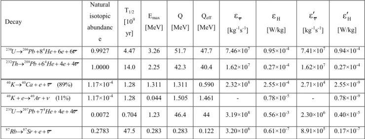
Geo-neutrinos are neutrinos produced in the decay chains of radioactive isotopes inside the Earth. To the present day few main nuclear isotopes (238U, 232Th, 40K, 235U and 87Rb) remained on the Earth. They have half-lives comparable or longer than Earth’s age. Actually neutrinos are produced only in electron capture of 40K. In contrast to Sun, Earth shines mainly antineutrinos. Main properties of these isotopes and (anti)neutrinos from them are summarized in Table 1.

Table 1. Properties of 238U, 232Th, 40K, 235U, and 87Rb and of (anti)neutrinos produced in their decay chains. For each nuclear isotope table presents the natural isotopic mass abundance, half-life, (anti)neutrino maximal energy. Q value, Q_eff Q E_{,} , antineutrino and heat production rates for unit mass of the isotope









MeV) are produced only in the decay chains of 238U, 232Th.

Decay Natural isotopic abundanc e T1/2 [109 yr] Emax [MeV] Q [MeV] Qeff [MeV] ν ε [kg-1_s-1_] H ε [W/kg] ν ε [kg-1_s-1_] H ε [W/kg]  6 6 84 206 238_{U Pb He e 0.9927 4.47 3.26 51.7 47.7 7.46×10}7 _0.95×10-4 _7.41×107 _0.94×10-4  4 4 64 208 232_{Th Pb He e} 1.0000 14.0 2.25 42.3 40.4 1.62×107 _0.27×10-4 _1.62×107 _0.27×10-4 %) 89 ( 40 40_{K Cae 1.17×10}-4 _{1.28 1.311 1.311 0.590 2.32×10}8 _2.55×10-4 _2.71×104 _2.55×10-9 %) 11 ( 40 40_{Ke Ar 1.17×10}-4 _{1.28 0.044 1.505 1.461 - 0.78×10}-5 _{- 0.78×10}-9  4 4 74 207 235_{U Pb He e} 0.0072 0.704 1.23 46.4 44 3.19×108 _0.56×10-3 _2.30×106 _0.40×10-5     Sr e Rb 87 87 _{0.2783 47.5 0.283 0.283 0.122 3.20×10}6 _0.61×10-7 _8.91×105 _0.17×10-7

The energy of antineutrinos from 87Rb is so low that unlikely their flux could be measured. Moreover heat production from Rb and some other rare elements (La, Lu, etc) account for the 1% of the total. Therefore only U, Th and 40K are considered further as the Heat

7 Producing Elements (HPEs) and unless otherwise specially stated geo-neutrinos refer to antineutrinos produced in the decay chains of these elements.

Geoneutrinos from different elements can be distinguished due to their different energy spectra, e.g. geoneutrinos with energy above 2.25 MeV can be produced only in 238U decay chain. The geoneutrino spectra are needed for calculation of the signal in a detector. Nowadays geoneutrinos are detected via inverse beta decay on free proton:

MeV 806 . 1     _{p e} _n e  (1.1)

where 1.806 MeV is a threshold of the reaction. Only neutrinos from 238U, 232Th (not those from

235_{U and} 40_{K) are above it. On these grounds the antineutrino energy spectra from} 238_{U and} 232_Th

decay chains are considered.

2.2 Geoneutrino spectra, cross section, oscillations

In general, the decay chain of an isotope involves many different β decays and the total antineutrino spectrum (in a case of radioactive equilibrium) results from the sum of the normalized individual spectra, with weights of production ratio of the isotopes and branching ratio of the beta decays. The detailed description of its calculation can be found in literature [Sanshiro, 2005, Fiorentini et al., 2007]. Here I present only general aspects of it.

The 238U decay chain has nine different β-decays Fig. 1. Only three of them (from 234Pa,

214_{Bi and} 210_{Tl) produce antineutrinos with energy larger than the threshold 1.806 MeV. The}

contribution from 210Tl is negligible, due to its small probability.

The 232Th decay chain has four β-decays Fig. 2. Only two of them (from 228Ac and 212Bi) produce antineutrinos with energy larger than the threshold 1.806 MeV.

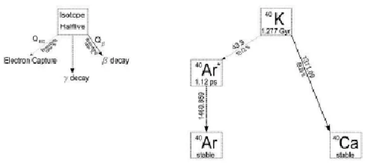
40_{K β-decay to} 40_{Ca. The simplified scheme is shown in Fig. 3. Antineutrinos from} 40_K

have lower energy than the threshold 1.806 MeV.

8 Fig. 1. The 238U decay chain [Fiorentini et al. 2007]. The two nuclides inside the grey boxes

(234Pa and 214Bi) are the main sources of geo-neutrinos.

Fig. 2. The 232Th decay chain [Fiorentini et al. 2007]. The two nuclides inside the grey boxes (228Ac and 212Bi) are the main sources of geo-neutrinos.

9 Fig. 3. Decay scheme of 40K [Fiorentini et al. 2007].

Fig. 4. Geo-neutrino spectra from U, Th and K decay chains. In this calculation, 82 beta decays in the U chain and 70 beta decays in the Th chain are considered. Neutrinos from 40K electron

capture are not shown in this figure. [Enomoto, 2005].

The total geoneutrino spectrum depends on the spectra of the individual decays, and on the abundances and spatial distribution of the HPE elements. In Fig. 5 it is shown for a specific model.

10 Fig. 5. Differential geo-neutrino luminosity, from [Enomoto, 2005]. One assumes the following global abundances: a(238U) =15 ppb, a(235U) = 0.1 ppb, a(232Th) = 55 ppb, a(40K) = 160 ppm [McDonough, 1999].

Geoneutrino cross section

A general discussion of neutrino/nucleon interaction cross section can be found in [Strumia and Vissani, 2003]. Here a simple approximation for the energies E_ 300MeV is considered:

,

,

]

[

10

)

(

_

_

_

_





p

cm

p

E

E

E

E

where Δ is the neutron-proton mass difference and all energies are in MeV. The uncertainty of cross section calculated by eq. (1.2) is 0.4%.

Calculation of geo-neutrino flux and signal

The number of geoneutrinos with energy E produced from the decay chain of element _

X (238U, 232Th) in time from a unit volume (dr) is:

 

r





_f

_E

_d

m

C

r

a

r

r

E

dN

_



(

)

(

)

)

(



11 where ρ – density, aX – elemental mass abundance, CX – isotopic concentration, τX –lifetime and

mX – mass of nucleus X. The energy distribution of antineutrinos fX

 

 



 dE_ f E_

n_{X X} . (1.4)

The geoneutrino flux decreases with distance as the inverse of square law and obtains by volume integration:

 













The flux arriving at detectors is smaller than produced due to neutrino oscillations. p





is the survival probability for antineutrino with energy E to reach the detector at _ R. Initially predicted theoretically, it was experimentally demonstrated in recent studies that neutrinos can change their flavor and at least two flavors have non zero masses.

        E R m P_ee 4 sin ) 2 ( sin 1 2 _ 2  2 _(1.6)

where δm is the difference of aqua red masses between two neutrinos, and θ is a mixing angle. The neutrino oscillation parameters δm and sin2(θ) are well determined be the recent studies [Fogli et al. 2011]. The survival probability averaged over a short distance with 1 σ uncertainty is equal to P_ee 0.5510.015 [Fogli et al. 2011] It gives







The measured signal depends on number of protons (Np), which have role of target in reaction

(1.1), detection efficiency ((E ) and cross section _) (E : _)



N  E_  E_ E_ dE_

X

S( ) _p ( ) ( ) _X( ) (1.8)

Assuming to have constant detection efficiency:



Calculation of an average cross section:

 





gives _(238_{U) 0.40410}44_cm2 _{and (}232_{Th) 0.12710}44_cm2_{. It results in ratio between}

12 ) ( ) ( ) (X N P X X S  _{p ee}   (1.11)

 

 









Signals are expressed in terms of a Terrestrial Neutrino Unit (TNU), defined as one event per 1032 target nuclei per year, or 3.17×10−40 s−1 per target nucleus. This unit is convenient, since, in practice, detectors, which utilize reaction (1.1) to measure antineutrino flux, contain about 1 kton of liquid scintillator. One kton of liquid scintillator contains about 1032 free protons (the precise value depending on the chemical composition) and the exposure times are of order of a few years.

2.3 Geoneutrinos and radiogenic heat generation

The total heat released from the Earth’s surface is believed to be between 30 and 46 TW [H.N.Pollack et al. 1993, A.M.Hofmeister, 2005, Jaupart et al., 2007]. Estimation is based on compilation of heat flow measurements at different sites. Where no observations are avaliable, heat flow is assumed to be the same as in the places with similar geological settings.

Different sources on the Earth may account for the released heat: radiogenic, gravitational, chemical, etc. According to existing BSE models, decay of radioactive elements contributes from 11 to 21 TW: 11 TW [Javoy et al. 2010], 16 TW [Lyubetskaya and Korenaga,

2007], 20 TW [McDonough and Sun, 1995], 21 TW [Palme and O’Neil, 2003].

Geochemical analysis evaluates the average abundances of HPEs in different layers of crust [Rudnick and Gao, 2003]. Seismic measurements determined thicknesses and densities of the layers [Bassin et al., 2000]. All together it allowed to estimate the mass of HPEs and released heat. On the ground of these data, the radiogenic heat production in the crust accounts for about 8 TW. The rest comes from the mantle and core.

The energy budget influences dynamics and thermal evolution of the Earth and observationally based determination of the radiogenic heat production would provide an important contribution for it understanding.

The minimal amount of radioactive elements in the Earth is the one compatible with lower bounds on measured abundances in the crust. In the same time, from available geochemical and/or geophysical knowledge, one cannot exclude that radioactivity in the present

13 Earth is enough to account for even the all terrestrial heat flow. This interval is rather large and can be reduced using geo-neutrino data. In fact, for each radioactive isotope there is a strict connection between the geoneutrino luminosity (L) (anti-neutrinos produced in the Earth per unit time), the radiogenic heat production rate (H) and the mass (m) of that isotope in the Earth [Fiorentini et al. 2007]: ) ( 16 . 23 ) ( 62 . 1 ) ( 49 . 31 ) ( 46 . 7 _m 238_{U m} 235_{U m} 232_{Th m} 40_K L        ) ( 85 . 2 ) ( 67 . 2 ) ( 53 . 55 ) ( 52 . 9 _m 238_{U m} 235_{U m} 232_{Th m} 40_K H_R        

where units are 1024 s-1, 1012 W, and 1017 kg respectively. Assuming to have natural isotopic abundances (Table 1), equations can be rewritten in terms of masses of these elements:

) ( 10 10 . 27 ) ( 62 . 1 ) ( 64 . 7 _{mU mTh} 4 _{m K} L        ) ( 10 33 . 3 ) ( 67 . 2 ) ( 85 . 9 _{mU mTh} 4 _{m K} H_R        

Thus after collecting required statistics geo-neutrino measurements would reduce allowed interval of radiogenic heat production in the Earth.

14

3 Global and local models for studying geoneutrinos in

Borexino

Deeper in the Earth, direct observations decrease dramatically, particularly, direct sampling of rocks for which geochemical data may be obtained. On the other hand, geoneutrinos are an extraordinary probe of the deep Earth. These particles carry to the surface information about the chemical composition of the whole planet and, in comparison with other emissions of the planet (e.g., heat or noble gases), they escape freely and instantaneously from the Earth’s interior.

The recent geoneutrino experimental results from KamLAND and Borexino detectors reveal the usefulness of analyzing the Earth’s geoneutrino flux, as it provides a constraint on the strength of the radiogenic heat power and this, in turn, provides a test of compositional models of the bulk silicate Earth (BSE). This flux is proportional to the amount and distribution of U and Th in the Earth’s interior.

A reference model (RM) for geo-neutrino production is a necessary starting point for studying the potential and expectations of detectors at different locations. It models the amount and distribution of neutrino sources inside the Earth. By definition, it should incorporate the best available geological, geochemical and geophysical information on our planet. In practice, it has to be based on selected geophysical and geochemical data and models (when available), on plausible hypotheses (when possible), and admittedly on arbitrary assumptions (when unavoidable) [Fogli et al., 2006].

In the last years several such models have been presented in the literature (Mantovani et al., 2004; Fogli et al., 2006; Enomoto et al., 2007; Dye 2010,). Review of these models is given in the next section. In general, geo-neutrino signal is calculated as a sum of contributions from three main reservoirs: crust, mantle and core.

Also a new RM is developed. Earth is considered as the sum of its metallic, silicate, and hydrospheric shells (see Fig. 1). The silicate shell of the Earth (equivalent to the BSE) is considered to be the main repository of U, Th and K, and attention is given on understanding internal differentiation of this region (Fig. 1). The BSE is composed of five dominant domains, or reservoirs: the DM (Depleted Mantle, which is the source of mid-ocean-ridge-basalts -- MORB), the EM (Enriched Mantle, which is the source of Ocean Island Basalts -- OIB), the CC (continental crust), the OC (oceanic crust), and the lithospheric mantle (LM). It follows that BSE = DM + EM + CC + OC + LM. The modern convecting mantle is composed of the DM and the

15 EM. We do not include a term for a hidden reservoir, which may or may not exist in the BSE; its potential existence is not a consideration of this paper.

Following the discussion in [McDonough, 2003], the Earth’s core is considered to have negligible amounts of K, Th and U.

Radiogenic heat production in the Earth is also determined by using developed reference model, because it is critical for understanding plate tectonics and the thermal evolution of the Earth.

16

3.1 Review of the previous estimations

Recently several reference models have been presented in the literature [Mantovani et al.,

2004, Fogli et al., 2005, Enomoto, 2005, Dye, 2010]. All these models rely on the geophysical 2°

× 2° crustal map of [Bassin et al., 2001, Laske et al. 2003] and on the density profile of the mantle as given by PREM [Dziewonski and Anderson, 1981].

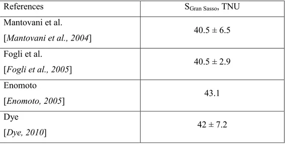
The geoneutrino signals at Gran Sasso National Laboratories predicted by these authors are compared in Table 3.1. Predicted signals are in good agreement with each other. The small differences are due to the adopted abundances of U and Th in the crust and upper mantle, and to the model of mantle. All papers use the BSE mass constraint in order to determine the abundances in the lower portion of the mantle.

Table 3.1. The geo-neutrino signal from U+Th at Gran Sasso area predicted by different authors.

References SGran Sasso, TNU

Mantovani et al. [Mantovani et al., 2004] 40.5 ± 6.5 Fogli et al. [Fogli et al., 2005] 40.5 ± 2.9 Enomoto [Enomoto, 2005] 43.1 Dye [Dye, 2010] 42 ± 7.2

17

3.2 Global model of the crust

Crust is a thin spherical shell on the top of the Earth. Its mass is negligible (about 0.5%) in the planetary scale. But, in spite of tiny volume and mass, crust contains about 40% of all radioactive elements presented in the Earth and contributes from 30% to 80% of the total geo-neutrino signal [Fiorentini et al. 2007]. Modern detectors are insensitive to directionality, and measure geo-neutrino flux generated from the whole planet (Crust+Mantle+Core). For the aim of the studying deep Earth one need to subtract contribution from the crust. Here the reference model of crust is build with the goal to encompass different published information and estimation of uncertainties, which comes from different constituents.

3.2.1 Geophysical model of the crust

All the previously considered reference models based their studies of crust on CRUST2.0 model of [Bassin et al. 2000]. CRUST2.0 has 16,200 tiles with resolution of 2°×2°. It was developed on refraction, reflection seismic measurements as an update of previously published 5°×5° CRUST5.1 model [Mooney et al., 1998]. Topography, bathymetry and thickness are given for each tile of 7 layers: ice, water, soft sediments, hard sediments, upper, middle and lower crust. Density and velocity of compressional (Vp) and shear waves (Vs) are determined for 360 key profiles for each tile. The Vp values are based on field measurements, while Vs and density are estimated by using empirical Vp-Vs and Vp-density relationships, respectively [Mooney et

al., 1998]. For regions lacking field measurements, the seismic velocity structure of the crust is

extrapolated from the average crustal structure for regions with similar crustal age and tectonic setting [Bassin et al., 2000]. Topography and bathymetry are adopted from a standard database (ETOPO-5). The same physical and elastic parameters are reported in a global sediment map digitized on a 1°×1° grid [Laske and Masters, 1997]. The accuracies of these models are not specified and they must vary with location and data coverage.

Evaluation of the uncertainties of the crustal structure is complex, as the physical parameters (thickness, density, Vp and Vs) are correlated, and their direct measurements are inhomogeneous over the globe [Mooney et al., 1998]. Seismic velocities generally have smaller relative uncertainties than thickness [Christensen and Mooney, 1995], since seismic velocities (Vp) are measured directly in the refraction method, while the depths of refracting horizons are successively calculated from the uppermost to the deepest layer measured. The uncertainties of seismic velocities in some previous global crustal models were estimated to be 3-4% [Holbrook

18

et al., 1992; Mooney et al., 1998]. To be conservative, 5% (1-sigma) uncertainties are adopted

for both Vp and Vs.

Fig. 3.1: Schematic drawing of the structure of the reference model (not to scale). Under the continental crust (CC; to the left of vertical dashed line), the lithospheric mantle (LM) from depleted mantle (DM), as discussed in the text is distinguished. The DM under the CC and the oceanic crust (OC) is assumed to be chemically homogeneous, but with variable thickness because of the depth variation of the Moho discontinuity as well as the continental lithospheric mantle. The boundary between DM and enriched mantle (EM) is determined by assuming that the mass of the enriched reservoir is 17% of the total mantle. The EM is a homogeneous symmetric shell between the DM and core mantle boundary (CMB).

In the reference model of Earth, presented here (see Fig. 3.1), the crust is digitalized on 1°x1° scale and consists of 8 reservoirs: ice, water, sediments 1, sediments 2, sediments 3, upper crust (UC), middle crust (MC) and lower crust (LC). Thicknesses of ice and water are well known and no uncertainties are associated with it. For each layer of crust model, the Vp, Vs, density and thickness are adopted for three sediment layers from the global sediment map [Laske

19 CRUST 2.0 [Bassin et al., 2000]. Thickness of crust is estimated from the comparison of different models, each crustal layer is proportionally rescaled. However thickness of CRUST2.0 gives reliable results and no significant geological discrepancies were found at 2°×2° scale, other existing models of crust obtained from different assumptions, are needed to be considered.

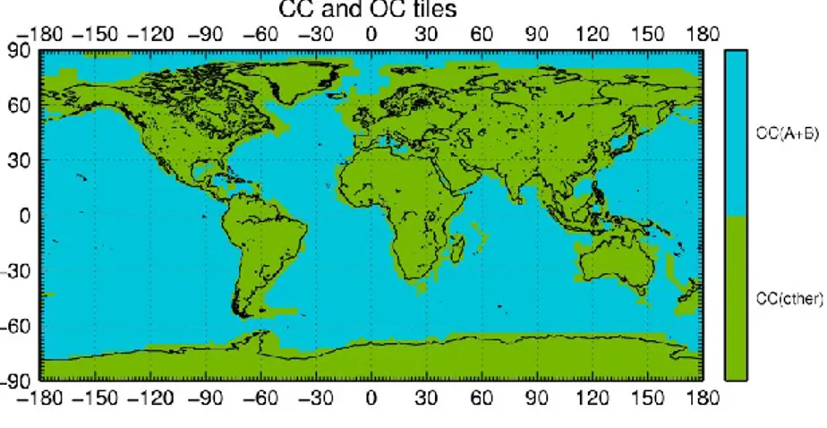
Determination of the CC-OC boundary is another crucial point. Amount of HPEs in the CC and OC crust can be several orders of magnitude different. The geo-neutrino signal, calculated for detectors placed far from the CC-OC boundary (SNO+, Hanohano, etc.), is not affected by small changes of its shape, but for others like KamLAND a movement of boundary can affect the final result. One way to obtain CC-OC boundary is to consider 360 key profiles of CRUST 2.0. Following [Huang et al. 2013] in the OC I include the oceanic plateaus and the melt affected oceanic crust of [Bassin et al. 2000]. The other crustal types identified in CRUST 2.0 are considered to be CC, including oceanic plateaus comprised of continental crust, which are mainly found in the north of the Scotia Plate, in the Seychelles Plate, in the plateaus around New Zealand (Campbell Plateau, Challenger Plateau, Lord Howe Rise and Chatham Rise), and on the northwest European continental shelf. The final 2°×2° map is presented in Fig. 3.2a. Another way can be based on gravimetrical measurements. The GOCE satellite (Gravity field and steady-state Ocean Circulation Explorer), launched in March, 2009, is the first gravity gradiometry satellite mission dedicated to providing an accurate and detailed global model of the Earth’s gravity field with a resolution of about 80 km and an accuracy of 1-2 cm in terms of geoid [Pail

et al., 2011]. The GEMMA project (GOCE Exploitation for Moho Modeling and Applications)

has developed the first global high-resolution map (0.5°×0.5°) of Moho depth by applying regularized spherical harmonic inversion to gravity field data collected by GOCE and preprocessed using the space-wise approach [Reguzzoni and Tselfes, 2009; Reguzzoni and

Sampietro, 2012]. This global crustal model is obtained by dividing the crust into different

geological provinces and defining a characteristic density profile for each of them. The gravity field is determined by multiplication of density with thickness. M. Reguzzoni and D. Sampietro have found that crossing of CC to OC is accompanied by a visible change of gravity. As a first approximation it can be considered as a boundary between CC and OC. Fig 3.2b shows the first 0.5°×0.5° map of CC-OC boundary obtained by this approach. The new countour decreases the mass of CC by 5%. The implication of the new CC-OC boundary on the geoneutrino signal needs to be studied in future. Here I consider determination of CC specified in CRUST 2.0, since all the previous models are based somehow on it.

20 (a)

(b)

Fig. 3.2 (a) CC-OC boundary determined on the ground of CRUST 2.0 model [Bassin et al.

2000]

(b) CC-OC boundary determined from gravity field measurements [Reguzzoni and Tselfes, 2009;

Reguzzoni and Sampietro, 2012].

The accuracy of the crustal thickness model is crucial to the calculations, as the uncertainties of all boundary depths affect the global crustal mass, the radiogenic heat power and the geoneutrino flux. In particular, uncertainties in Moho depths are a major source of uncertainty in the global crustal model. Although CRUST 2.0 does not provide uncertainties for global crustal thickness, the previous 3SMAC topographic model [Nataf and Richard, 1996] included the analysis of crust-mantle boundary developed by [Čadek and Martinec 1991], in

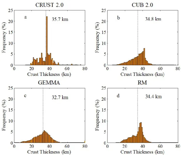
21 which the average uncertainties of continental and oceanic crustal thickness are 5 km and 3 km (1-sigma), respectively. Fig. 3.3a shows the dispersion of the thickness of all CC voxels in CRUST 2.0. The surface area weighted average continental and oceanic crustal thickness (ice and water excluded, sediment included) in CRUST 2.0 is 35.7 km and 7.5 km, respectively (Table 3.3). Distribution of crustal thicknes in CRUST 2.0 model is presented in Fig. 3.4a.

Fig. 3.3: Distributions of continental crustal thickness (without ice or water) in three global crustal models and the reference model (RM). The average thicknesses of the four models, as shown by the dots lines, are calculated from surface area weighted averaging, and so do not coincide with the mean of the distribution. CRUST 2.0: Laske et al. [2001]; CUB2.0: Shapiro

and Ritzwoller [2002]; GEMMA: Negretti et al. [2012].

The gravimetric method can be used to check the crustal thickness of CRUST2.0. It is particularly valuable because crustal density cannot be directly determined from seismic refraction field measurements [Mooney et al. 1998, Tenzer 2009]. Using the database of GEMMA [Negretti et al., 2012], the surface area weighted average thicknesses of CC and OC are 32.7 km and 8.8 km (Table 3.3), respectively (Fig. 3.3b, Fig 3.4b).

22 Another way to evaluate the global crustal thickness is by utilizing the phase and group velocity measurements of the fundamental mode of Rayleigh and Love waves. [Shapiro and

Ritzwoller 2002] used a Monte Carlo method to invert surface wave dispersion data for a global

shear-velocity model of the crust and upper mantle on a 2°×2° grid (CUB 2.0), with a priori constraints (including density) from the CRUST 5.1 model [Mooney et al., 1998]. The surface area weighted average thicknesses of the CC and OC are 34.8 km and 7.6 km, respectively (Fig. 3.3c, Fig. 3.4, Table 3.3).

The three global crustal models described above were obtained by different approaches and the constraints on the models are slightly dependent. Ideally, the best solution for a geophysical global crustal model is to combine data from different approaches: reflection and refraction seismic body wave, surface wave dispersion, and gravimetric anomalies. In the reference model the thickness and its associated uncertainty of each 1°×1° crustal voxel is obtained as the mean and the half-range of the three models. The surface area weighted average thicknesses of CC and OC are 34.4 ±4.1 km (Fig. 2d, Fig3.5) and 8.0±2.7 km (1-sigma) for our reference crustal model, respectively. The uncertainties reported here are not based on the dispersions of thicknesses of CC and OC voxels, but are the surface area weighted average of uncertainties of each voxel’s thickness. The estimated average CC thickness is about 16% less than 41 km determined previously by [Christensen and Mooney 1995] (see their Fig. 3.3) on the basis of available seismic refraction data at that time and assignment of crustal type sections for areas that were not sampled seismically. However, their compilation did not include continental margins, nor submerged continental platforms, which are included in the three global crustal models used here. Inclusion of these areas will make the CC thinner, on average, than that based solely on exposed continents.

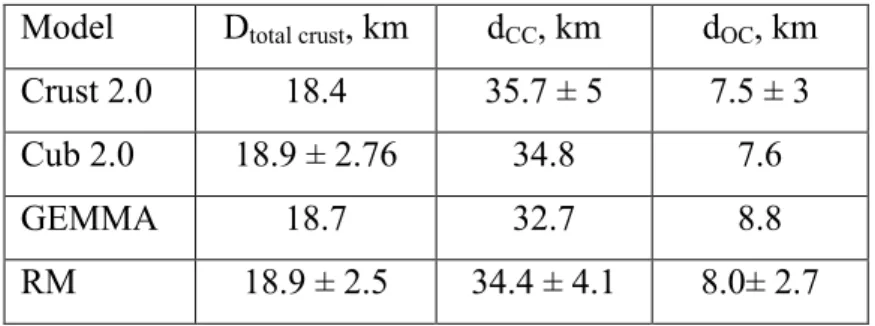
Table 3.2. Thickness of crust and its 1 σ uncertainty (where available) in different models. Model Dtotal crust, km dCC, km dOC, km

Crust 2.0 18.4 35.7 ± 5 7.5 ± 3

Cub 2.0 18.9 ± 2.76 34.8 7.6

GEMMA 18.7 32.7 8.8

RM 18.9 ± 2.5 34.4 ± 4.1 8.0± 2.7

The calculated thickness and mass of crust for all layers are presented in Table 3.3. Summing the masses of sediment, upper, middle and lower crust, the total masses of CC and OC are estimated to be MCC = (20.6±2.5) ×1021 kg and MOC = (6.7±2.3) ×1021 kg (1-sigma). Thus,

23 the fractional mass contribution to the BSE of the CC is 0.51% and the contribution of the OC is 0.17%. The uncertainty of crustal thickness of one cell is correlated somehow with the others, since the three crustal models are mutually dependent, and the estimates of crustal thicknesses for some cells are extrapolated from the others. Considering these complexities, a conservative assumption was made, the uncertainty of Moho depth in each cell is totally dependent on that of all the others.

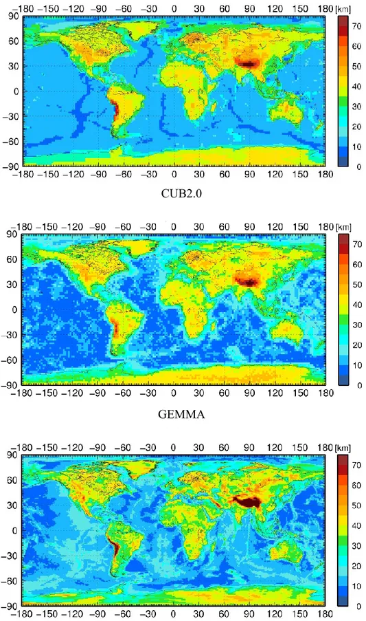
24 CRUST 2.0

CUB2.0

GEMMA

Fig. 3.4 Distributions of crustal thickness (without ice or water) in three global crustal models. CRUST 2.0: Laske et al. [2001]; CUB2.0: Shapiro and Ritzwoller [2002]; GEMMA: Negretti et

25 Table 3.3: Global average physical (density, thickness, mass and radiogenic heat power) and chemical (abundance and mass of HPEs) properties of each reservoir as described in the reference model. The BSE model is based on [McDonough and Sun 1995] and [Arevalo et al. 2009]. The physical structure of BSE above and beneath the Moho is based on this study and PREM, respectively. The uncertainty in density is about the same as that of Vp (3-4%) [Mooney et al., 1998]. We adopt a simple model for the mantle and do not report any uncertainties for its properties. [Sramek et al. 2012] review different mantle models and predict the consequences to the surface geoneutrino flux.

ρ, g/cm3 d, km M, 10 21 _kg Abundance Mass H, TW U, μg/g Th, μg/g K, % U, 1015 kg Th, 10 15 kg K, 10 19 _kg CC Sed 2.25 1.5±0.3 0.7±0.1 1.73±0.09 8.10±0.59 1.83±0.12 0.2 0.2 1.2  5.81.11.1   1.30.20.2   0.30.10.1   UC 2.76 11.6±1.3 6.7±0.8 2.7±0.6 10.5±1.0 2.32±0.19 4.8 4.3 18.2  70.7 10.710.2   15.62.32.1   4.20.70.6   MC 2.88 11.4±1.3 6.9±0.9 0.58 0.36 0.97  4.864.302.25   0.81 0.52 1.52  6.64.12.5   33.330.015.5   10.45.73.7   0.9 0.6 1.9  LC 3.05 10.0±1.2 6.3±0.7 0.14 0.07 0.16  0.961.180.51   0.650.340.22   1.00.90.4   6.07.73.3   4.12.21.4   0.40.30.1   LM 3.37 140±71 97±47 0.05 0.02 0.03  0.150.280.10   0.030.040.02   2.9 5.42.0   14.529.49.4   3.14.71.8   0.81.10.6   OC Sed 2.03 0.6±0.2 0.3±0.1 1.73±0.09 8.10±0.59 1.83±0.12 0.2 0.2 0.6  0.9 0.9 2.8  0.2 0.2 0.6  0.1 0.1 0.2  C 2.88 7.4±2.6 6.3±2.2 0.07±0.02 0.21±0.06 0.07±0.02 0.2 0.2 0.4  1.30.70.5   0.4 0.20.2   0.10.040.03   DM 4.66 2090 3207 0.008 0.022 0.015 25.7 70.6 48.7 6.0 EM 5.39 710 704 0.034 0.162 0.041 24.0 113.7 28.7 6.3 BSE 4.42 2891 4035 0.020 0.079 0.028 80.7 318.8 113.0 20.1

26

3.2.2 Composition of the crust

Crust is an onliest reservoir which can be directly sampled. Its composition can be estimated better than of the other reservoirs.

Compositional estimates for some portions of the crust are adopted from previous work, whereas the composition of the deep continental crust is re-evaluated.

Sediments: The average composition of sediments and uncertainties are adopted from the GLOSS II model (GLObal Subducting Sediments) [Plank, 2013].

Oceanic Crust: An average oceanic crust composition is adopted from [White and Klein

2013] with a conservative uncertainty of 30%. The three seismically defined layers of basaltic

oceanic crust reported by [Mooney et al. [1998] is treated as one reservoir.

Upper Continental Crust: The compositional model reported by [Rudnick and Gao 2003] for the upper continental crust and the uncertainties are adopted. Following [Mooney et al. 1998], the upper continental crust is defined seismically as the uppermost crystalline region in CRUST 2.0, having an average Vp of between 5.3 and 6.5 km s-1.

Middle and Lower Crust: Composition of these layers was calculated following [Huang

et al. 2013]. The correlation between seismic velocities and rock types was used for quantitative

estimates of deep crustal composition and associated uncertainties. Middle and lower CC are assumed to be a binary mixture of felsic and mafic rocks.

Intermediate rocks, which have intermediate seismic velocities compared to those of felsic and mafic rocks, are not considered. As pointed out by [Rudnick and Fountain 1995], the very large range in velocities makes determination of their deep crustal abundances using seismic velocities impossible. It is assumed that a negligible amount of intermediate rocks is hidden in the deep crust. Since they have higher abundances of HPEs than mafic rocks and similar HPE contents to felsic rocks, ignoring their presence may lead to an underestimation of HPEs in the deep continental crust. Thus, estimates perfumed here should be regarded as minima.

At room temperature and 600 MPa pressure, amphibolite facies felsic rocks and mafic amphibolites, which represent felsic and mafic rocks in middle crust, have an average Vp of 6.34±0.16 km/s and Vp of 6.98±0.20 km/s (1-sigma) respectively. Granulite-facies felsic rocks and mafic granulites (felsic and mafic rocks in lower crust) have average Vp of 6.52±0.19 km/s and 7.21±0.20 km/s (see Table 3.4).

Because seismic velocities of rocks in the deep crust are strongly influenced by pressure and temperature, the laboratory-measured velocities for all rock groups (which were attained at

27 0.6 GPa and room temperature) were corrected to seismic velocities appropriate for pressure-temperature conditions in the deep crust. The pressure and pressure-temperature derivatives of 2 × 10-4 km s-1 MPa-1 and -4 × 10-4 km s-1 ºC-1 were applied respectively [Christensen and Mooney, 1995;

Rudnick and Fountain, 1995], and assume a typical conductive geotherm equivalent to a surface

heat flow of 60 mW·m-2 [Pollack and Chapman, 1977]. Using the in situ Vp and Vs profiles for the middle (or lower) CC of each voxel given in CRUST 2.0, the fractions of felsic and mafic rocks were evaluated:

1   m f (Eq. 3.1) f m crust f v  m v v (Eq. 3.2)

where f and m are the mass fractions of felsic and mafic end members in the middle (or lower) CC; vf, vm and vcrust are Vp or Vs of the felsic and mafic end members (pressure- and

temperature- corrected) and in the crustal layer, respectively. Only Vp is used to constrain the felsic fraction (f) in the middle or lower CC for three main reasons: using Vs gives results for (f) in the deep crust that are in good agreement with those derived from the Vp data, the larger overlap of Vs distributions for the felsic and mafic end-members in the deep crust limits its usefulness in distinguishing the two end-members [Huang et al. 2012], and Vs data in the crust are deduced directly from measured Vp data in CRUST 2.0.

The distributions of the HPE abundances in felsic and mafic amphibolite and granulite facies rocks are taken from compilation of [Huang et al. 2012] and presented in Table 3.4 with associated 1 σ uncertainties. These values were calculated on the basis of compositional databases of representative rocks. The abundances have asymmetrical uncertainties due to log-normal distribution of the applied fit.

Table 3.4. Average laboratory-measured Vp (600 MPa, room temperature) and HPE abundances in amphibolite facies, granulite facies and peridotite rocks with 1σ uncertainty.

Rock type Vp, km/s K2O, wt.% Th, μg/g U, μg/g Amphibolite Facies (MC) Felsic 6.34±0.16 1.81 11 . 1 89 . 2   8.27 84..1210   1.37 10..0359   Mafic 6.98±0.20 0.41 23 . 0 50 . 0 _ 0.57 29 . 0 58 . 0 _ 0.39 19 . 0 37 . 0 _ Granulite Facies (LC) Felsic 6.52±0.19 2.05 17 . 1 71 . 2 _ 7.53 54 . 2 87 . 3 _ 0.41 21 . 0 42 . 0 _ Mafic 7.21±0.20 0.31 17 . 0 39 . 0   0.3000..4618 0.1000..0614

28

3.2.3 Calculation of amount of HPE and geoneutrino signal from the crust

Calculated amount of HPEs (Table 3.3), which determines the radiogenic heat power and geoneutrino signal is based on the physical (density and thickness) and chemical (abundance of HPEs) characteristics of each crustal layer in the reference model. For the middle and lower CC, Vp and composition of amphibolite and granulite facies rocks were used to determine the average abundance of HPEs, as it was discussed:

f m

a f a  m a (Eq. 3.3)

where af and am is the abundance of HPEs in the felsic and mafic end member, respectively; a is

the average abundance in the reservoir. Equations 3.1 and 3.2 define the mass fractions of felsic and mafic end members (f and m) in the MC and LC reservoirs. In the rare circumstance when the calculated average abundance is more (or less) than the felsic (or mafic) end member, it is assumes that the average abundance should be the same as the felsic (or mafic) end member. The calculated radiogenic heat power is a direct function of the masses of HPEs and their heat production rates: 9.85×10-5, 2.63×10-5 and 3.33×10-9 W/kg for U, Th and K, respectively [Dye,

2012].

The distribution of HPEs in these different reservoirs affects the geoneutrino flux on the Earth’s surface. Summing the antineutrino flux produced by HPEs in each volume of the model, the geoneutrino unoscillated flux (unosc.) expected in Gran Sasso area can be calculated. The flux from U and Th arriving at detectors is smaller than that produced, due to neutrino oscillations, (osc.)

U, Th = <Pee> (unosc.)U, Th, where <Pee> = 0.55 is the average survival probability

[Fiorentini et al., 2012]. The geoneutrino event rate in a liquid scintillator detector depends on the number of free protons in the detector, the detection efficiency, the cross section of the inverse beta reaction, and the differential flux of antineutrinos from 238U and 232Th decay arriving at the detector. Taking into account the U and Th distribution in the Earth, energy distribution of antineutrinos [Fiorentini et al., 2010], the cross section of inverse beta reaction [Bemporad et al., 2002], and mass-mixing oscillation parameters [Fogli et al., 2011], the geoneutrino event rate from the decay chain of 238U and 232Th at the site of Borexino detector was computed (Table 3.5). For simplicity, the finite energy resolution of the detector is neglected, and 100% detection efficiency is assumed. The expected signal is expressed in TNU.

29 Table 3.5. Geoneutrino signal at the site of Borexino detector from each reservoir as described in the reference Earth model. The unit of signal is TNU as defined in Section 3.1. The reported uncertainties are 1 σ. ROC is defined as Rest of Crust with the geoneutrino signal originated from the 24 closest 1°×1° crustal voxels excluded from the total crustal signal (see Section 3.3).

Borexino 42.45 N, 13.57 E S(U) S(Th) S(U+Th) Sed_CC 0.3 0.3 1.3_ 0.09 0.09 0.4_ 0.3 0.3 1.8_ UC 3.6 3.4 13.7  3.7 0.60.5   17.53.63.4   MC 3.3 1.8 4.7  1.81.70.9 7.03.92.5 LC 0.8 0.4 1.0_ 0.9 0.3 0.5_ 1.3 0.7 1.7_ CLM 2.7 1.0 1.4  0.41.00.3   2.23.11.3   Sed_OC 0.06 0.05 0.2_ 0.02 0.02 0.06_ 0.1 0.1 0.2_ OC 0.02 0.02 0.05  0.010.0050.004   0.060.020.02   Bulk Crust 5.2 4.6 21.4  6.82.31.4 29.06.05.0 ROC 10.3 2.62.2   3.2 1.10.7   13.7 2.82.3   Total LS 6.8 5.2 23.6  7.62.91.8   31.97.35.8   DM 4.1 0.8 4.9 EM 2.7 0.8 3.5 Grand Total 7.3 5.8 40.2  --

30

3.2.4 Estimation of uncertainties

Estimation of the uncertainties in the reference model is not straightforward. The commonly used quadratic error propagation method [Bevington and Robinson, 2003] is only applicable for linear combinations (addition and subtraction) of errors of normally distributed variables. For non-linear combinations (such as multiplication and division) of uncertainties, the equation provides an approximation when dealing with small uncertainties, and it is derived from the first-order Taylor series expansion applied to the output. Moreover, the error propagation equation cannot be applied when combining asymmetric uncertainties (non-normal distributions). Because of this, the most common procedure for combining asymmetric uncertainties is separately tracking the negative error and the positive error using the error propagation equation. This method has no statistical justification and may yield the wrong approximation.

To trace the error propagation in the reference model, MATLAB was used to perform a Monte Carlo simulation [Huang et al., 2012; Robert and Casella, 2004; Rubinstein and Kroese,

2008]. Monte Carlo simulation is suitable for detailed assessment of uncertainty, particularly

when dealing with larger uncertainties, non-normal distributions, and/or complex algorithms. The only requirement for performing Monte Carlo simulation is that the probability functions of all input variables (for example, the abundance of HPEs, seismic velocity, thickness of each layer in the reference model) are determined either from statistical analysis or empirical assumption. Monte Carlo analysis can be performed for any possible shape probability functions, as well as varying degrees of correlation. The Monte Carlo approach consists of three clearly defined steps using MATLAB. The first step is generating large matrices with pseudorandom samples of input variables according to the specified individual probability functions (Here 105 random numbers were enough to achieve stable result after series of iterations). Then the output variable (such as mass of HPEs, radiogenic heat power and geoneutrino flux) is calculated from the matrixes that are generated following the specified algorithms function. The final step is to do statistical analysis of the calculated matrix for the output variable (evaluation of the distribution, central value and uncertainty).

31

3.2.5. Discussion

Physical and Chemical Structure of the Reference Crustal Model

The thickness of the reference crustal model is obtained by averaging the three geophysical global crustal models obtained from different approaches, as described in Section 3.2.1. The distributions of crustal thickness and associated relative uncertainty in the model are shown in Figs. 3.5a and 3.5b, respectively. The uncertainties of the continental crustal thickness are not homogeneous: platform, Archean and Proterozoic shields, the main crustal types composing the interior of stable continents and covering ~50% surface area of the whole CC, have thickness uncertainties rarely exceeding 10%, while the thickness of continental margin crust is more elusive. Larger uncertainties for the thickness estimates occur in the OC, especially for the mid ocean ridges (Fig. 3.5b). The average crustal thicknesses (including the bulk CC, bulk OC and different continental crustal types) and masses of the reference model are compared with the three geophysical models. The global average thicknesses of platforms, Archean and Proterozoic shields are all previously estimated to be 40-43 km [Christensen and Mooney, 1995;

Rudnick and Fountain, 1995]. Although GEMMA yields the thinnest thicknesses for shields and

platforms, considering that the typical uncertainty in estimating global average CC thickness is more than 10% [Čadek and Martinec, 1991], the reference model, as well as the other three crustal models, fall within uncertainty of estimates by [Christensen and Mooney 1995] at the 1-sigma level. Extended crust and orogens in the three input models and in the average model show average thicknesses higher than, but within 1 σ of the estimations made by [Christensen

and Mooney 1995]. The surface area weighted average thicknesses of bulk CC for the three input

models and our reference model are smaller than the ~41 km estimated by [Christensen and

Mooney 1995], likely due to the fact that they did not include continental margins, submerged

continental platforms and other thinner crustal types in their compilation. The thickness of OC is generally about 7-8 km, with the exception of the GEMMA model, which yields 8.8 km thick average OC. The possible reason for the thick OC in GEMMA is due to the poorly global density distribution under the oceans. However, considering that the average uncertainty in determining the crustal thickness in the oceans is about 2-3 km [Čadek and Martinec, 1991], the three input models yield comparable results.

32 (a)

(b)

33 (a)

(b)

Fig. 3.6. The abundance of U in the middle (a) and lower (b) CC obtained by using seismic velocity argument.

34 As shown in Fig. 3.6 the middle and lower CC of the reference model are compositionally heterogeneous on a global scale. The average middle CC derived here has

0.58 0.36 0.97_ g/g U, 4.30 2.25 4.86_ g/g Th and 0.81 0.52

1.52_ wt.% K, while the average abundances of U, Th and K in the lower CC are 0.14

0.07 0.16  g/g, 0.96 1.180.51   g/g and 0.65 0.340.22   wt.%, respectively (Table

3.6; Fig. 3.6). The uncertainties reported for the new estimates of the HPE abundances in the deep crust are significantly larger than reported in previous global crustal geochemical models [e.g., Rudnick and Fountain, 1995; Rudnick and Gao, 2003], due to the large dispersions of HPE abundances in amphibolite and granulite facies rocks.

Because of these large uncertainties, all of the estimates for HPEs in the deep crust of the reference model agree with most previous studies at the 1 σ level (Table 3.6). For the middle CC, the central values of estimates for HPEs are generally only ~10% to 30% lower than those made by [Rudnick and Fountain 1995] and [Rudnick and Gao 2003]. For the lower CC, the difference in HPEs between this model and several previous studies is significantly larger than that of the middle CC. The reference model has lower U and Th, but higher K concentrations, agreeing at the 1 σ level, than the previous estimates of the lower CC by [Rudnick and Fountain 1995] and [Rudnick and Gao 2003]. Taylor and McLennan [Taylor and McLennan 1995], McLennan [McLennan 2001], Wedepohl [Wedepohl 1995] and Hacker et al. [Hacker et al. 2011] constructed two-layer crustal models with the top layer being average upper CC (from either their own studies, or [Rudnick and Gao 2003] in the case of [Hacker et al. 2011]) and the bottom layer equal to the average of the middle and lower CC in the reference model presented here (see Fig. 3 in [Hacker et al. 2011]). The abundances of U, Th and K in the combined middle and lower CC of this model are 0.32

0.20 0.60  g/g, 3.22 2.351.35   g/g, and 1.14 0.450.32   wt.%, respectively, which

agrees within 1 σ uncertainty of the estimates of [Hacker et al. 2011] and within uncertainty of the Th and U abundances of [McLennan 2001] and of K abundance of [Wedepohl 1995], but are significantly higher than the abundance estimates of [Taylor and McLennan 1995] for all elements, and the K abundance estimate of [McLennan 2001], while lower than the Th and U abundances of [Wedepohl, 1995]. Similarly, for the bulk CC, estimates of HPE abundances presented here are close to those determined by [Rudnick and Fountain 1995], and [Rudnick and

Gao 2003]. Obtained results also agree with those of [Hacker et al. 2011], though their Th

concentration is at the 1 σ upper bound of our model. By contrast, the reference model has significantly higher concentrations of HPEs, beyond the 1 σ level, than estimates by [McLennan

2001] and [Taylor and McLennan 1995], and lower than estimates by [Wedepohl 1995]. The

35 and 28%, respectively, of their total amount in the BSE [McDonough and Sun, 1995]. The estimates of the K/U ( 3,512

2,516

11,656_ ) and Th/U ( 1.6 1.0

4.4_ ) in the bulk CC agree with all previous studies at the 1-σ level, due to the large uncertainties associated these two ratios derived from large uncertainties of HPE abundance in the CC.

Geoneutrino Flux and Radiogenic Heat Power

In the past decade different authors have presented models for geoneutrino production from the crust, and associated uncertainties. Mantovani et al. [Mantovani et al., 2004] adopted minimal and maximal HPE abundances in the literature for each crustal layer of CRUST 2.0 in order to obtain a range of acceptable geoneutrino fluxes. Based on the same geophysical crustal model, Fogli et al. [Fogli et al.,2006] and Dye [Dye, 2010] estimated the uncertainties of fluxes based on uncertainties of the HPE abundances reported by [Rudnick and Gao, 2003].

Fig. 3.7 shows the map of geoneutrino signal at Earth’s surface. The reference model was built to estimate the 1 σ uncertainties of geoneutrino fluxes and radiogenic heat power taking into account two main sources of uncertainties: the physical structure (geophysical uncertainty) and the abundances of HPEs in the reservoirs (geochemical uncertainty). This approach allowed to evaluate the geophysical and geochemical contributions to the uncertainties of the model, particularly for the lithosphere. With respect to the previous estimates the asymmetrical distribution of the uncertainties as a consequence of the non-Gaussian distributions of HPE abundances in the deep CC and CLM was pointed out. Within 1 σ uncertainties, obtained results for U and Th geoneutrino signal from the crust predicted for Borexino detector (Table 3.5) is comparable to that reported by [Mantovani et al., 2004] and [Dye, 2010], for which symmetrical and homogeneous uncertainties were adopted. Reported in Table 3.5 asymmetrical 1 σ uncertainties of the geoneutrino signal are a consequence of the detailed characterization of the crustal structure and its radioactivity content.

The different contributions from geophysical and geochemical uncertainties to the 1-σ uncertainties of total crustal geoneutrino signals were studied. In the developed reference model the total predicted signal for Borexino is 6.0

5.0

29.0_ TNU. Fixing the HPE abundances in all crustal reservoirs constant at their central values, uncertainties associated with the geophysical model contribute ±2.7 TNU to the total uncertainties of the crustal geoneutrino signal at Borexino. By fixing the crustal thickness of all voxels constant, the geochemical uncertainties contribute 5.0

4.3  

36 TNU to the total uncertainties crustal geoneutrino signal at Borexino. The geochemical uncertainties clearly dominate the total uncertainty of the crustal geoneutrino signals.

Precise estimation of crustal contribution to the total geoneutrino signal together with experimental measurement of the signal would provide constraints on permissible BSE compositional models [Dye, 2010; Fiorentini et al., 2012; Sramek et al., 2012]. In particular, by subtracting the predicted crustal signal (Scrust) from the experimental total rates (Stot, exp), it is

expected to infer the mantle contributions (Smantle). Furthermore, refined model of the crustal

structure in the region close to the detector gives the uncertainty of the signal from LOcal Crust (SLOC, see next section 3.3), which reduce the uncertainty of global crustal signal [Coltorti et al.,

2011]. Since Scrust in this study is the sum of SLOC and SROC (the signal from the Rest Of the

Crust after excluding local crust), Table3.5 reports the geoneutrino signal SROC (expected from

Rest Of Crust + CLM) on the base of the reference model of all crust. In the next future all these calculations and experimental measurements of geoneutrino flux at different sites on the Earth surface can be used for extracting the mantle geoneutrino signals, following this equation:

Smantle = Stot, exp – SROC – SLOC.

The CC in the reference model contributes 1.4 1.1

7.0

 TW radiogenic heat power to the total

20.1 TW radiogenic power generated in the considered BSE, which agrees with previous estimates by Hacker et al. [Hacker et al., 2011], Rudnick and Fountain [Rudnick and

Fountain,1995], and Rudnick and Gao [Rudnick and Gao, 2003] and at the 1 σ level, but is

higher than estimates by McLennan [McLennan, 2001] and Taylor and McLennan [Taylor and

McLennan, 1995], and lower than estimate by Wedepohl [Wedepohl, 1995] (Table 3.6). The

geophysical and geochemical contribution of to the total uncertainties of radiogenic heat power were estimated, they are: ±0.8 TW and 1.1

0.8 

 TW at 1-σ respectively.

Although the mass of OC (excluding the overlying sediment) is poorly known, its contribution to the anticipated geoneutrino signals is less than 0.2 TNU at the 1-σ level.

37 Fig. 3.7. Geoneutrino signal at Earth’s surface. The unit is TNU.

Table 3.6. Estimates of the K, Th and U concentrations and radiogenic heat power (P) in the continental crust. K, Th and U concentrations are listed as wt. %, μg/g, and μg/g, respectively, P in TW (1012 W). Keys to models: TM [Taylor and McLennan, 1995]; M [McLennan, 2001]; W [Wedepohl, 1995]; H [Hacker et al., 2011]; RF [Rudnick and Fountain, 1995]; RG [Rudnick and

Gao, 2003]. Radiogenic heat power is calculated from the bulk CC assuming it has a mass of

20.6×1021 kg as developed here reference model.

TM M W H RF RG RM Upper Crust K 2.8 2.8 2.87 _{2.32 2.8 2.32±0.19 2.32±0.19} Th 10.7 10.7 10.3 _{10.5 10.7 10.5±1.0 10.5±1.0} U 2.8 2.8 2.5 2.7 2.8 2.7±0.6 2.7±0.6 Middle Crust K - - - - 1.67 1.91 0.81 0.52 1.52_ Th - - - - 6.1 6.5 4.30 2.25 4.86  U - - - - 1.6 1.3 0.97 0.580.36   Lower Crust K 0.28 0.53 1.31 1.24 0.50 0.50 0.34 0.22 0.65_ Th 1.06 2.0 6.6 5.6 1.2 1.2 1.18 0.51 0.96  U 0.28 0.53 0.93 0.7 0.2 0.2 0.16 0.140.07   Bulk CC P 5.6 6.3 8.5 7.9 7.7 7.4 6.81.14.1

38

3.3 Local model of the crust

The major contribution to geo-neutrino signal comes from the region close to the detector due to its proximity. For KamLAND and Borexino, Mantovani et al. [Mantovani et al., 2004] estimated that about one half of the signal originates from an area surrounding the detector within a radius of 400 km and 800 km, respectively (Fig. 3.8). This region, although containing a globally negligible amount of U and Th, produces a large contribution to the signal as a consequence of its proximity to the detector.

100

km

200

km

200

km

100

km

Fig. 3.8 (a) 50% of the total geo-neutrino signal in Borexino originates within 900 km around detector; (b) 50% of the total geo-neutrino signal in KamLAND originates within 600 km around detector.

39 Current reference models [Mantovani et al., 2004, Fogli et al. 2005, Enomoto 2007, Dye

2010] for the Earth’s crust use the map of [Bassin et al. 2000] divided into 2°x 2°horizontally homogeneous tiles, which is clearly a very rough approximation for describing the region surrounding the detector. Moreover, worldwide averages for the chemical composition of different regions of the Earth (e.g., upper crust, lower crust, and mantle) are used to estimate U and Th concentrations. However, if one wants to extract from the total signal relevant information on the deep Earth, the regional/local contribution needs to be determined on the grounds of a more detailed geological, geochemical and geophysical study of the region. The reasonable refinement of the model supposes that the local contribution to the geo-neutrino signal needs to be determined with an accuracy that is comparable to the uncertainties from the contributions of the rest of the Earth.

This highlights the need for a detailed study for the region around detector, which improves the accuracy of the reference model. Such a study was performed in [Fiorentini et al.,

2005; Enomoto et al., 2007] for Kamioka; a refined reference model for Gran Sasso is presented

in this chapter.

According to the reference model [Mantovani et al. 2004] the total predicted geo-neutrino signal at Gran Sasso area is 40.5 TNU. The last column of Table 3.7 shows the contributions of the different reservoirs to the signal in this model. The mantle contributes 9 TNU, about 20% of the total signal, while crust and sediments all over the world provide the rest of the contribution (31.5 TNU). Half of this originates from the six tiles depicted in Fig. 3.9 which provide a “local contribution”:

Sreg =15.3 TNU

Within this region, the 2° x 2° Central Tile, indicated as CT in Fig. 3.9, generates a “local contribution” of:

SCT =11.8 TNU

Geological units and structures, which present in the detector area, might be washed out in the 2°×2° crustal map. To improve the knowledge of this region a three dimensional (3D) geological model of the 2°x 2° area around Gran Sasso was build. It is based on the results of a deep seismic exploration of the Mediterranean and Italy (the CROP project) [Finetti, 2005a], as well as geological and stratigraphical distribution of the sedimentary covers (SC) recognizable from geological maps, integrated with data from deep oil and gas wells. The main feature of this area is a thick sedimentary cover, which was not adequately accounted for in the averages leading to the 2° x 2° crustal map