Waste management analysis in developing countries through unsupervised classification of mixed data

¥

Article

Waste Management Analysis in Developing Countries

through Unsupervised Classification of Mixed Data

Department of Philosophical, Pedagogical and Economic-Quantitative Sciences, University G. d’Annunzio Chieti-Pescara, Vle Pindaro n. 42, 65127 Pescara, Italy; gattone@unich.it

* Correspondence: giulia.caruso@unich.it

Received: 7 May 2019; Accepted: 6 June 2019; Published: 13 June 2019

Abstract: The increase in global population and the improvement of living standards in developing countries has resulted in higher solid waste generation. Solid waste management increasingly represents a challenge, but it might also be an opportunity for the municipal authorities of these countries. To this end, the awareness of a variety of factors related to waste management and an efficacious in-depth analysis of them might prove to be particularly significant. For this purpose, and since data are both qualitative and quantitative, a cluster analysis specific for mixed data has been implemented on the dataset. The analysis allows us to distinguish two well-defined groups. The first one is poorer, less developed, and urbanized, with a consequent lower life expectancy of inhabitants. Consequently, it registers lower waste generation and lower CO2emissions. Surprisingly, it is more

engaged in recycling and in awareness campaigns related to it. Since the cluster discrimination between the two groups is well defined, the second cluster registers the opposite tendency for all the analyzed variables. In conclusion, this kind of analysis offers a potential pathway for academics to work with policy-makers in moving toward the realization of waste management policies tailored to the local context.

Keywords: cluster analysis; unsupervised classification; mixed data; circular economy; waste management

1. Introduction

In recent years, the term circular economy has gained much attention. It refers to a system of production and consumption providing minimal losses of materials and energy through extensive reuse, recycling, and recoveryHaupt et al.(2017). In other words, it is an economic system for which is essential to recycle materials from waste in order “to close the cycle”.

Furthermore, the increase in global population and the improvement of living standards in developing countries has resulted in higher solid waste generation in the areas under investigation Abarca-Guerrero et al. (2013); Minghua et al. (2009). Consequently, nowadays waste management is at the center of a very lively debate Fernández-González et al. (2017);

Schneider et al.(2017).

Waste disposal should be gradually eliminated, and where this is not possible, it should be monitored in order to be safe for human health and the environment. Consequently, solid waste management increasingly represents a challenge since municipalities must provide an efficient system to their population. However, they often have to struggle with complexity and with lack of both organization and financial resourcesBurntley(2007).

Among other things, sustainable waste management is able to reduce the incidence of health problems, the emission of greenhouse gases, and the deterioration of landscape, water, and air caused by landfillingCucchiella et al.(2017). However, it not only represents a contribution to environmental

protection, but it also pays off economicallyNelles et al.(2016): waste management practices, indeed, can be cost-saving and generate revenue opportunitiesRomero-Hernández and Romero(2018).

In fact, waste can be a useful source of raw materials and energy, too. Metals, glass, and textiles have long been collected and put to new use; for example, the extraction of nickel and cobalt from raw materials, as well as from waste, is strategically important for industry and society

Komnitsas et al.(2019). Waste can be turned into energy too, enabling the value of products, materials, and resources to be maintained on the market for as long as possible, minimizing waste and resource use in the wake of the objectives of circular economyMalinauskaite et al.(2017).

For all these reasons, and since the circular economy is an important issue for the future and the competitiveness of businessesGarcia-Muiña et al.(2018), solid waste management might represent an opportunity for the municipal authorities of developing countries, especially those characterized by a low-incomeMinghua et al.(2009).

In conclusion, in a circular economy wastes are considered a resource, especially from an economic point of view, consequently attracting an increasing number of industrial actors, policy-makers, and researchersCucchiella et al.(2017). Thus, in the last years, a large number of studies have tried to detect factors influencing waste management systems in developing countries.

Therefore, since the awareness of a variety of factors related to waste management might prove to be particularly significantGhinea and Gavrilescu(2019);Zeller et al.(2019);Zohoori and Ghani(2017), this paper aims to analyze some of them in the developing countries involved in the study.

From our analysis, it may be concluded that a study of this kind offers a potential pathway for academics to work with policy-makers in moving toward the realization of waste management policies tailored to the local context.

2. Materials and Methods

Real data often consists of mixed variables, that is, both continuous and categorical ones; an example is provided by the dataset analyzed in this paper, produced byAbarca-Guerrero(2014), the variables of which are described in Table 1. Traditionally, cluster analysis has only focused on datasets composed of a single type of variable (all quantitative or all qualitative). For this reason, researchers dealing with mixed data usually convert them into a single data type, transform the categorical variables into binary ones and consequently apply methods for numeric variables, or transform continuous variables into categorical onesDougherty et al.(1995);

Ichino and Yaguchi(1994).

Indeed, clustering methods specific to mixed data are less encountered in the literature. Some traditional methods are:

• data pre-processing, that is, all variables are converted to the same scale, either numerical to categorical or vice-versa;

• distance measures specifically developed for mixed datasets.

With regards to data pre-processing, these algorithms are essentially created for purely categorical attributes, although they have also been applied to mixed data after a transformation of numerical attributes to categorical ones (discretization). In general, these kinds of algorithms can be applied to mixed data through a discretization process that may, nevertheless, produce a loss of important informationCaruso et al.(2018).

One example is represented by the dummy coding of all categorical variables. But this increases the dataset’s dimensionality, representing a problem when the number of categorical variables simultaneously increases with the size of the data. Another disadvantage is that any semantic similarity in the original dataset is lost in the transformed one. Finally, coding strategies imply a difficult choice of weights representing categorical attributesFoss et al.(2016).

An alternative to recoding categorical or continuous variables is to use a dissimilarity measure, taking into account the different types of dataCaruso(2019). A common approach is to use the Gower distanceGower(1971).

2.1. Clustering Mixed Data

Let X = {x1, x2, . . . , xn}denote a set of n objects and xi = [xi1, xi2, . . . , xiL] indicate an object

constituted by L variables. Since the L variables of the considered dataset are both continuous and categorical, it is possible to write L=Q+C, where Q corresponds to the number of numeric variables and C to the number of categorical ones.C = {lC₁, . . . lC_C}is a subset identifying the qualitative variables andQ = {lQ₁, . . . lQ_Q}is a subset denoting the quantitative ones. The aim of clustering is to assign the n objects contained in X to K separate clusters. When clustering mixed datasets, the main problem is to determine how close or how far apart objects are from each other.

There are different approaches presenting different ways to combine distance measures for numerical variables and distance measures for categorical ones into a single cost functionCaruso

(2019);Caruso et al.(2019,in printb);Everitt(1974);Huang(1997). 2.2. The Huang Method

Huang(1998) presented a so-called K-prototypes algorithm, which is based on the K-means method but overcomes its quantitative data limitation, preserving, at the same time, its efficiency. The algorithm groups the objects in clusters against k prototypes. The updates occur in a dynamical manner, so as to minimize the following objective function:

E= K

∑

∑

where uikis an element of a partition matrix Un×k, andΦH(xi, Vk)is a dissimilarity measure for mixed

data between the objects xiand Vk.

Vk= [vk1, vk2, . . . , vkL]is the prototype or representative vector for cluster k. U represents a hard

partition matrix, where uik∈ {0, 1}, and uik=1 if xiis allocated to cluster k.

The Huang dissimilarity measure for mixed data is defined as ΦH(xi, Vk) =

∑

l∈Q

(xil−vkl)2+γk

∑

δ(xil, vkl), (2)

where the first term is the squared Euclidean distance, whereas the second one is defined as δ(r, t) =0 for r=t and δ(r, t) =1 for r6=t. γkis a weight for categorical variables in cluster k.

The internal term in Equation (1) can be defined as Ek = n

∑

i=1

uikS(xi, Vk). It measures the total

dissimilarity of objects in cluster k from their prototype Vk. The quantity Ekcould be considered as the

total cost of allocating the objects xi(i∈Ck)to cluster k.

This term may be rewritten as Ek = n

∑

∑

∑

∑

where EQ_k and EC_k represent the dissimilarity of the objects in cluster k for the quantitative and the qualitative variables, respectively. In order to minimize these two components, let V_kQand V_kCbe the prototypes for cluster k for the numerical and categorical variables, respectively.

E_kQis minimized with the usual update of the K-means algorithm for continuous variables. That is, the generic component of V_kQis the arithmetic mean:

vkl= 1 nk n

∑

where nkis the number of objects in cluster k. LetWl = {wl,1, wl,2, . . . , wl,ml}be the set enclosing the

distinct values of the l-th categorical variable, and let pl(wl,j|k)be the probability that value wl,jis

observed in cluster k.

It is possible to rewrite EC_k in (3) as EC_k =

∑

l∈C

nk[1−p(vkl∈ Wl|k)] . (5)

In Equation (5), E_kCis minimized by selecting the categorical values of the prototype W_kC, such that p(vkl∈ Wl|k) ≥p(wlj ∈ Wl|k)for vkl6=wl,jfor all categorical variables.

On the basis of the Huang algorithm, by minimizing (1), we implemented a cluster analysis with a number of clusters equal to K=2. This choice was made based on the Silhouette indexRousseeuw

(1987); since higher values corresponds to better results, the resultant (optimal) maximum value precisely corresponds to 2.

3. Results 3.1. The Dataset

The datasetAbarca-Guerrero(2014) used in this application has been extracted from the data archive of the “4TU.Centre for Research Data” in the Netherlands, and it regards the period of 1985–2011. It contains information on factors influencing the municipal waste management system in 22 developing countries; each of these is associated with more than one observation.

The dataset considers some key factors affecting waste management systems, in particular the country performance in terms of public health (life expectancy at birth), economy (gross domestic product/capita/year), and environment (CO2-emissions/capita).

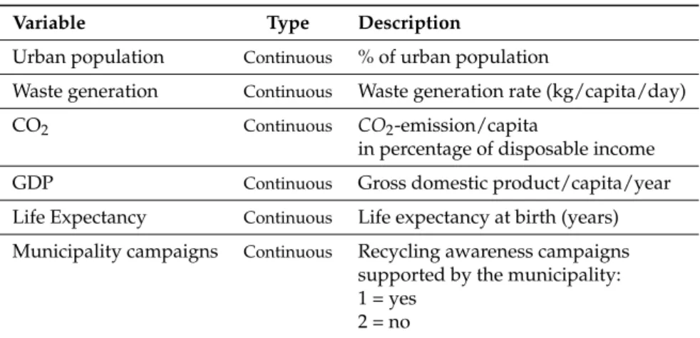
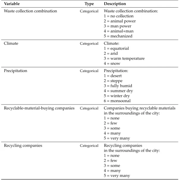
Other general parameters characterizing the countries are the urban population, the kind of climate, and precipitation. Furthermore, waste-specific parameters have been considered: the waste generation rate (kg/capita/day) and the sophistication of waste collection. The latter can be articulated as 1 = no organized collection of solid waste; 2 = collection based on manpower only; 3 = collection based on both manpower and draught animal; 4 = collection based on motorized transport but no compactor used; and 5 = collection based on motorized transport and compactor used. Other parameters include the existence of a recycling culture and the presence of municipality awareness campaigns, of recyclable-material-buying companies, and of recycling companies, the latter two specifically in the surroundings of the city. In conclusion, the analyzed data consist of a selection of 11 variables (6 continuous and 5 categorical), described in detail in Table 1, for a total of 50 observationsAbarca-Guerrero(2014).

Table 1.Description of all of the analyzed variables.

Variable Type Description

Urban population Continuous % of urban population

Waste generation Continuous Waste generation rate (kg/capita/day) CO2 Continuous CO2-emission/capita

in percentage of disposable income GDP Continuous Gross domestic product/capita/year Life Expectancy Continuous Life expectancy at birth (years) Municipality campaigns Continuous Recycling awareness campaigns

supported by the municipality: 1 = yes

Table 1. Cont.

Variable Type Description

Waste collection combination Categorical Waste collection combination: 1 = no collection

2 = animal power 3 = man power 4 = animal+man 5 = mechanized Climate Categorical Climate:

1 = equatorial 2 = arid

3 = warm temperature 4 = snow

Precipitation Categorical Precipitation: 1 = desert 2 = steppe 3 = fully humid 4 = summer dry 5 = winter dry 6 = monsoonal

Recyclable-material-buying companies Categorical Companies buying recyclable materials in the surroundings of the city:

1 = none 2 = few 3 = some 4 = many 5 = very many Recycling companies Categorical Recycling companies

in the surroundings of the city: 1 = none 2 = few 3 = some 4 = many 5 = very many 3.1.1. Internal Indexes

Since the ground truth (i.e., an empirical evidence)Han et al.(2011) is not given for this dataset, it is not possible to compute the external indexes. The internal ones are shown below.

We compared several methods for clustering mixed data types, namely those of:Huang(1997),

Ahmad and Dey(2007), andCheung and Jia(2013).

The relevant validity of cluster results was evaluated through the above-mentioned indexes and the Huang method proved to be the one yielding the best results, namely the highest values of the Calinski–Harabasz index (CH)Calinski and Harabasz(1974) and of the Silhouette index (SHI)

Rousseeuw(1987), both computed on quantitative variables. The results provided by these methods are shown in Table2.

Table 2.Internal indexes. CH—Calinski–Harabasz index; SHI—Silhouette index.

Method CH SHI

Huang 13.23 0.21

Ahmad & Dey 10.15 0.209

3.1.2. Analysis of Quantitative Variables

First of all, we provide the descriptive analysis of the quantitative variables used: the mean, the standard deviation, and the values corresponding to the 1st, the 2nd, and the 3rd quartiles, as shown in Table3.

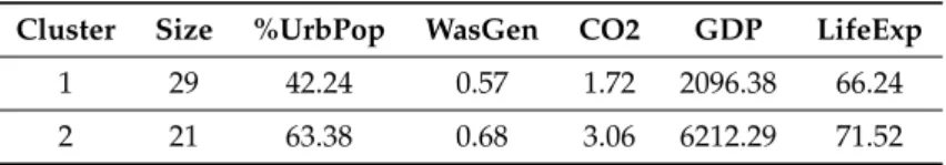
Table4displays, for each cluster, the mean value of the analyzed quantitative attributes. With regards to the variable “waste generation”, the two groups have a weak cluster structure, that is clusters values are very similar between them, whereas they have a strongest structure with regards to the variable “GDP”. With regards to the “percentage of urban population”, the relevant overall mean equals 51.12. Thus, the first cluster mean is lower than the average one, whereas the second one is higher. For what concerns the “waste generation rate”, instead, the overall mean corresponds to 0.61. In this case as well, the first cluster mean is lower than the overall one, whereas the second one is higher. However, in this case the separation between clusters is less marked. With regards to the “CO2emissions”, the overall mean value is 2.28, so the first cluster mean is lower than the overall one,

whereas the second one is higher. For what concerns the “GDP”, the overall mean value is equal to 3825, so the first cluster mean is lower than the average, whereas the second one is significantly higher. With regards to “life expectancy”, the overall mean equals 68.46; in this case as well, the first mean is lower and the second one is higher. In summary, for all of the analyzed quantitative variables, the first cluster is below the overall mean whereas the second cluster overcomes it.

Table 3.Descriptive statistics of quantitative variables.

Variables Mean Standard Deviation Q1 Q2 Q3

%UrbPop 51.12 19.35 33.50 57 65.75

WasGen 0.61 0.28 0.41 0.50 0.82

CO2 2.28 2.51 0.80 1.40 3.50

GDP 3825 6747.90 1069 2349 4469

LifeExp 68.46 8.27 66 71 73

Table 4.Mean values of quantitative variables for each cluster.

Cluster Size %UrbPop WasGen CO2 GDP LifeExp

1 29 42.24 0.57 1.72 2096.38 66.24 2 21 63.38 0.68 3.06 6212.29 71.52

3.1.3. Analysis of Qualitative Variables

Table5shows the overall distribution of the variable “municipality campaigns”. The prevailing modality is represented by the presence of recycling awareness campaigns supported by the municipality. Table 6, instead, shows more in detail the distribution of the categorical variable “municipality campaigns” for each of the two clusters. The first one, which has the strongest cluster structure, is characterized by the presence of recycling awareness campaigns supported by the municipality, whereas the second cluster is characterized by their absence.

Table 5.Overall distribution of the categorical variable “municipality campaigns”.

Municipality Campaigns Distribution

Yes 0.68

Table 6.Distribution of the categorical variable “municipality campaigns”.

Municipality Campaigns Clusters

1 2

Yes 0.90 0.38 No 0.10 0.62

Table 7 shows the overall distribution of the variable “waste collection combination”. The prevailing modality is represented by “animal power”, followed by “mechanized methods”.

In Table8, the two clusters are clearly outlined. In the first, the prevailing modality is represented by “animal power”, whereas in the second one it corresponds to “mechanized” methods. By comparing the obtained clusters with the relevant overall distribution, the first cluster registers a higher use of methods based on “animal power” than in the overall distribution. The same applies to the modality “mechanized” methods in the second cluster.

Table 7.Overall distribution of the categorical variable “waste collection combination”.

Waste Collection Combination Distribution

No collection 0.02

Animal power 0.42

Man power 0.12 Animal + man 0.12

Mechanized 0.32

Table 8.Distribution of the categorical variable “waste collection combination”.

Waste Collection Combination Clusters

1 2 No collection 0.00 0.05 Animal power 0.66 0.10 Man power 0.17 0.05 Animal + man 0.00 0.29 Mechanized 0.17 0.52

Table 9 shows the overall distribution of the variable “climate”. The modality with the overwhelming majority is “equatorial”.

Table10shows that in both clusters, the prevailing modality is represented by the modality “equatorial”, in the wake of the overall distribution.

Table 9.Overall distribution of the categorical variable “climate”.

Climate Distribution

Arid 0.18

Equatorial 0.72

Snow 0.02 Warm 0.08

Table 10.Distribution of the categorical variable “climate”. Climate Clusters 1 2 Arid 0.17 0.19 Equatorial 0.76 0.67 Snow 0.03 0.00 Warm 0.03 0.14

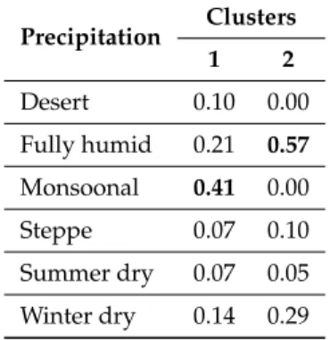
Table11, instead, shows the overall distribution of the variable “precipitation”. The prevailing modality is represented by “fully humid”.

In Table12, the distribution of the two clusters is shown. The first cluster is characterized by the prevalence of the modality “monsoonal”, whereas in the second cluster the most frequent modality is “fully humid”, exactly like in the overall distribution.

Table 11.Overall distribution of the categorical variable “precipitation”.

Precipitation Distribution Desert 0.06 Fully humid 0.36 Monsoonal 0.24 Steppe 0.08 Summer dry 0.06 Winter dry 0.20

Table 12.Distribution of the categorical variable “precipitation”.

Precipitation Clusters 1 2 Desert 0.10 0.00 Fully humid 0.21 0.57 Monsoonal 0.41 0.00 Steppe 0.07 0.10 Summer dry 0.07 0.05 Winter dry 0.14 0.29

Table13shows the overall distribution of the variable “recyclable-material-buying companies”. The prevailing modality is represented by “some”.

In Table14, the distribution of the two clusters is shown. The first cluster is characterized by a prevalence of the modality “some”, exactly as in the overall distribution, whereas in the second cluster the most frequent modality is “none”.

Table15shows the overall distribution of the variable “recycling companies in the surroundings of the city”. The prevailing modality is represented by “none”.

In Table16, the distribution of the two clusters is shown. The first cluster has a prevalence of the modality “some”, whereas in the second cluster the most frequent modality is “none”, exactly as in the overall distribution.

Table 13.Overall distribution of the categorical variable “recyclable-material-buying companies”.

Recyclable-Material-Buying Companies Distribution

none 0.28

few 0.18

some 0.38

many 0.16

very many 0.00

Table 14.Distribution of the categorical variable “recyclable-material-buying companies”.

Recyclable-Material-Buying Companies Clusters

1 2 none 0.00 0.67 few 0.10 0.29 some 0.62 0.05 many 0.28 0.00 very many 0.00 0.00

Table 15.Overall distribution of the categorical variable “recycling companies in the surroundings of

the city”.

Recycling Companies Distribution

none 0.34

few 0.30

some 0.24

many 0.10

very many 0.02

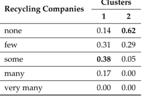
Table 16.Distribution of the categorical variable “recycling companies in the surroundings of the city”.

Recycling Companies Clusters

1 2 none 0.14 0.62 few 0.31 0.29 some 0.38 0.05 many 0.17 0.00 very many 0.00 0.00 4. Discussion

On the basis of our analysis of quantitative variables, it appears that the first cluster is characterized by a lower percentage of urban population, lower levels of GDP, and a lower life expectancy. As a consequence of limited urbanization and greater poverty, this group registers lower rates of waste generation and of CO2 emissions. Since the cluster discrimination between

the two groups is well defined, the second cluster registers the opposite tendency for all of the above-mentioned variables, namely higher levels of GDP and a stronger percentage of urban population, with a consequently higher life expectancy. The higher urbanization corresponds to higher levels of waste generation and of CO2emissions. In more detail, in order to better describe the

distribution of the quantitative variables analyzed, each of these has been represented through a box plotCleveland(1993).

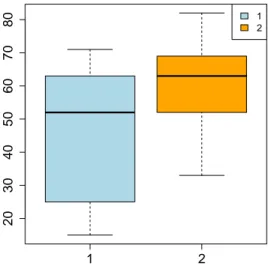
With regards to the percentage of urban population (Figure 1), the overall median of the distribution equals 57.00, whereas the overall mean is 51.12; the mean of the first cluster is lower than this, whereas the one associated with the second cluster is higher. In the first cluster, the interquartile distance is much higher than in the second one, denoting a greater dispersion of the 50% most central observations around the median. On the other hand, since the interquartile distance of the second cluster is lower, the 50% most central observations are highly concentrated around the median. Furthermore, since in the first cluster the distances between each quartile and the median are quite different from one another, the distribution is asymmetric. In the second cluster, instead, the distances are more similar between these, denoting a lower asymmetry of the distribution.

1 2 20 30 40 50 60 70 80 1₂

Figure 1.Boxplot of the variable “urban population” in clusters 1 and 2.

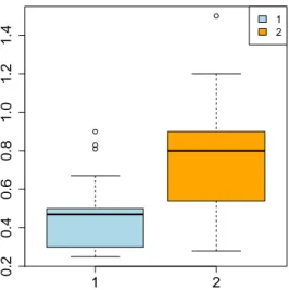
For what concerns the waste generation (Figure2), the overall median of the distribution equals 0.50, whereas the overall mean is 0.61; the mean of the first cluster is lower than this, whereas the one associated with the second cluster is higher. In the first cluster, the interquartile distance is lower than in the second one. Thus, in the first group there is a low dispersion of the 50% most central observations around the median. On the other hand, since the interquartile distance of the second cluster is higher, the 50% most central observations are less concentrated around the median. Furthermore, in the first cluster the two distances are quite different from one another, denoting a very asymmetric distribution, whereas in the second group these distances are more similar, resulting in a slightly lower asymmetry of the distribution.

With regards to the CO2emissions (Figure3), the overall median of the distribution equals 1.40,

whereas the overall mean is 2.28; the mean of the first cluster is lower than this, whereas the one associated to the second cluster is higher. In the first cluster, the interquartile distance is lower than in the second one. Thus in the first group, the dispersion of the 50% most central observations around the median is lower. On the other hand, since the interquartile distance of the second cluster is higher, the 50% most central observations are less concentrated around the median. Furthermore, in the first cluster the two distances are very similar to one another, denoting a symmetric distribution, whereas in the second cluster they are less similar, indicating the asymmetry of the distribution.

1 2 0.2 0.4 0.6 0.8 1.0 1.2 1.4 1 2

Figure 2.Boxplot of the variable “waste generation” in clusters 1 and 2.

1 2 0 2 4 6 8 10 12

Figure 3.Boxplot of the variable “CO2” in clusters 1 and 2.

With regards to the GDP (Figure4), the overall median of the distribution equals 2349, whereas the mean is 3825; the median of the first cluster is lower than this, whereas the one associated with the second cluster is higher. In the first cluster, the interquartile distance is lower than in the second one. Thus, in the first group the dispersion of the the 50% most central observations around the median is lower. Since the interquartile distance of the second cluster is higher, instead, the 50% most central observations are less concentrated around the median. Furthermore, in the first cluster the two interquartile distances are quite different from one another, so the distribution is asymmetric. In the second cluster, instead, they are more similar, denoting the lower asymmetry of the distribution.

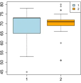
For what concerns life expectancy (Figure5), the overall median of the distribution equals 71.00, whereas the overall mean is 68.46, thus the mean of the first cluster is lower than this, whereas the one associated with the second cluster is higher. In the first group, the interquartile distance is higher than in the second one. Thus, in the first group the dispersion of the 50% most central observations around the median is higher. On the other hand, since the interquartile distance of the second cluster is lower, the 50% most central observations are highly concentrated around the median. Furthermore, in the first cluster the two distances are quite different from one another, so the distribution is asymmetric, whereas in the second group the distances are more similar, denoting the lower asymmetry of the distribution.

1 2 2000 4000 6000 8000 1 2

Figure 4.Boxplot of the variable “GDP” in clusters 1 and 2.

1 2 45 50 55 60 65 70 75 80 1 2

Figure 5.Boxplot of the variable “life expectancy” in clusters 1 and 2.

With regards to qualitative variables, instead, the first cluster is characterized by the overwhelming majority of recycling awareness campaigns supported by the municipality, the waste is mainly collected through animal power, and there are some recyclable-material-buying companies and some recycling companies in the surrounding areas of the cities. The countries falling under this category are mostly characterized by monsoonal precipitation and are the following: Ethiopia, Sri Lanka, Thailand, China, Peru, Tanzania, India, Bangladesh, Nepal, Malawi, Zambia, Nicaragua, Kenya, and the Philippines.

The second cluster, instead, is mainly characterized by the absence of recycling awareness campaigns supported by the municipality, the waste is mainly collected through mechanized tools, but it is mostly characterized by the absence of recyclable-material-buying companies and of recycling companies in the surrounding areas of the cities. Furthermore, it is characterized by the prevalence of a fully humid climate. The countries falling into this cluster are Turkey, Suriname, Costa Rica, Ecuador, Pakistan, and Bhutan, whereas Indonesia and South Africa are in the overlapping area of the two clusters.

5. Conclusions

Since nowadays more and more applications are based on datasets composed of mixed data, there is an ever-growing interest in cluster analysis. Due to their characteristics, traditional methods are unable to capture, store, manage, and analyze these datasets. A cluster analysis implemented on such

a dataset has huge potential; however, most clustering algorithms are designed to exclusively handle one type of data at a time, being unable to analyze mixed data simultaneously. The use of cluster analysis for mixed data represents an element of innovation, especially in the waste management sector, since until now only the traditional cluster analysis has been applied in this framework.

Certainly, the research in this area is far from being complete. There are quite a few methods in the literature, but further advancements in this field are neededCaruso(2019). Furthermore, in the wake of this work, future research will be focused on the development of new cluster analysis techniques for mixed data and on the consequent creation of dedicated software packages, also with the aim of widening the number of potential users of this methodCaruso et al.(2019).

The basis for future developments will take into consideration the results yielded from the applications described in Section3and from an interesting insight provided by the work of Diday and GovaertDiday and Govaert(1977). They propose an adaptive clustering that consists in a dynamic procedure and is useful for calibrating the weights of variables used in the clustering.

Usually, indeed, all of the variables participate in the cluster analysis with the same importance, but since some of them may be more discriminant than others, or better characterize a cluster, there are some ways to correctly consider their different valuesIrpino et al.(2016).

One strategy consists in assigning a weight to each variable in advance, on the basis of a prior knowledge, and then performing a cluster analysis; a future development could consist in computing the weights for each variable in an automatic wayCaruso(2019). In this context, Diday and GovertDiday and Govaert(1977) proposed using an adaptive distance when clustering real data. It is necessary to introduce a weighting step in the optimization process, generating a set of weights; each of these corresponds to a variable and measures its importance in the cluster analysis. While Diday and Govert’s proposal is only focused on quantitative variables, a further advancement could be to extend it to both quantitative and qualitative data.

Furthermore, an additional input for our future research could be to extend this kind of analysis to our recent studyCaruso et al.(in printa). Moreover, since clustering is also at the center of a very lively debateDi Battista et al.(2016),Di Battista and Fortuna(2016),Fortuna and Maturo(2018),

Fortuna et al.(2018) in the functional framework, a further and interesting possible development could be to also consider this kind of approach in our future research.

Author Contributions:Conceptualization G.C.; methodology G.C.; software, G.C.; formal analysis, G.C.; data

curation, G.C.; supervision, S.A.G.

Funding:This research received no external funding.

Conflicts of Interest:The authors declare no conflict of interest.

References

Abarca-Guerrero, Lilliana. 2014. Municipal Waste Management Data Set. Eindhoven University of Technology. Available online: https://doi.org/10.4121/uuid:31d9e6b3-77e4-4a4c-835e-5c3b211edcfc (accessed on 6 June 2019).

Abarca-Guerrero, Lilliana, Ger Maas, and William Hogland. 2013. Solid waste management challenges for cities in developing countries. Waste Management 33: 220–32. [CrossRef] [PubMed]

Ahmad, Amir, and Lipika Dey. 2007. A k-mean clustering algorithm for mixed numeric and categorical data. Data & Knowledge Engineering 63: 503–27.

Burntley, Stephen. 2007. A review of municipal solid waste composition in the United Kingdom. Waste Management Journal 27: 1274–85. [CrossRef] [PubMed]

Calinski, Tadeusz, and Joachim Harabasz. 1974. A dendrite method for cluster analysis. Communications in Statistics 3: 1–27.

Caruso, Giulia. 2019. Cluster Analysis for Mixed Data. Ph.D. Dissertation, University G. d’Annunzio Chieti-Pescara, Chieti, Italy.

Caruso, Giulia, Stefano Antonio Gattone, Francesca Fortuna, and Tonio Di Battista. 2018. Cluster Analysis as a Decision-Making Tool: A Methodological Review. In Decision Economics: In the Tradition of Herbert A. Simon’s Heritage. Advances in Intelligent Systems and Computing. Edited by Edgardo Bucciarelli, Shu-Heng Chen and Juan Corchado. Berlin: Springer International Publishing, Vol. 618, pp. 48–55.

Caruso, Giulia, Stefano Antonio Gattone, Antonio Balzanella, and Tonio Di Battista. 2019. Cluster analysis: An application to a real mixed-type data set. In Models and Theories in Social Systems. Studies in Systems, Decision and Control. Edited by Cristina Flaut, Sarka Hoskova-Mayerova and Daniel Flaut. Berlin: Springer International Publishing, Vol. 179, pp. 525–33.

Caruso, Giulia, Tonio Di Battista, and Stefano Antonio Gattone. In printa. A micro-level analysis of regional economic activity through a PCA approach. In Decisions Economics: Complexity of Decisions and Decisions for Complexity. Advances in Intelligent Systems and Computing. Edited by Edgardo Bucciarelli, Shu-Heng Chen and Juan Corchado. Berlin: Springer International Publishing.

Caruso, Giulia, Stefano Antonio Gattone, Francesca Fortuna, and Tonio Di Battista. In printb. Cluster Analysis for mixed data: An application to credit risk evaluation. In Book of Short Papers IES 2019. Advances in Intelligent Systems and Computing. Edited by Matilde Bini, Pietro Amenta, Antonello D’Ambra and Ida Camminatiello. Naples: Cuzzolin.

Cheung, Yiu-ming, and Hong Jia. 2013. Categorical-and-numerical-attribute data clustering based on a unified similarity metric without knowing cluster number. Pattern Recognition 46: 2228–38. [CrossRef]

Cleveland, William. 1993. Visualizing Data. New York: Murray Hill.

Cucchiella, Federica, Idiano D’Adamo, Massimo Gastaldi, Lenny Koh, and Paolo Rosa. 2017. A comparison of environmental and energetic performance of European countries: A sustainability index. Renewable and Sustainable Energy Reviews 78: 401–13. [CrossRef]

Di Battista, Tonio, and Francesca Fortuna. 2016. Clustering dichotomously scored items through functional data analysis. Electronic Journal of Applied Statistical Analysis 9: 433–50.

Di Battista, Tonio, Angela De Sanctis, and Francesca Fortuna. 2016. Clustering functional data on convex function spaces. In Studies in Theoretical and Applied Statistics, Selected Papers of the Statistical Societies. Berlin: Springer, pp. 105–14.

Diday, Edwin, and Gerard Govaert. 1977. Classification Automatique avec Distances Adaptatives. R.A.I.R.O. Informatique Computer Science 11: 329–49.

Dougherty, James, Ron Kohavi, and Mehran Sahami. 1995. Supervised and unsupervised discretization of continuous features. In Machine Learning: Proceedings of the Twelfth International Conference, Tahoe City, CA, USA, July 9–12. San Francisco: Morgan Kaufmann Publishers, pp. 194–202.

Everitt, Brian. 1974. Cluster Analysis. London: Heinemann Educational Books Ltd.

Fernández-Gonzalez, Jose-Manuel, Alejandro Luis Grindlay, Francisco Serrano-Bernardo, Maria Isabel Rodríguez-Rojas, and Montserrat Zamorano. 2017. Economic and environmental review of Waste-to-Energy systems for municipal solid waste management in medium and small municipalities. Waste Management 67: 360–74. [CrossRef]

Fortuna, Francesca, and Fabrizio Maturo. 2018. K-means clustering of item characteristic curves and item information curves via functional principal component analysis. Quality and Quantity [CrossRef]

Fortuna, Francesca, Fabrizio Maturo, and Tonio Di Battista. 2018. Clustering functional data streams: Unsupervised classification of soccer top players based on Google trends. Quality and Reliability Engineering International 34: 1448–60. [CrossRef]

Foss, Alex, Marianthi Markatou, Bonnie Ray, and Aliza Heching. 2016. A semiparametric method for clustering mixed data. Machine Learning 105: 419–58. [CrossRef]

Garcia-Muiña, Fernando, Rocio González-Sánchez, Anna Maria Ferrari, and Davide Settembre-Blundo. 2018. The Paradigms of Industry 4.0 and Circular Economy as Enabling Drivers for the Competitiveness of Businesses and Territories: The Case of an Italian Ceramic Tiles Manufacturing Company. Social Sciences 7: 255. [CrossRef]

Ghinea, Cristina, and Maria Gavrilescu. 2019. Solid Waste Management for Circular Economy: Challenges and Opportunities in Romania—The Case Study of Iasi County. In Towards Zero Waste. Greening of Industry Networks Studies. Edited by Maria-Laura Franco-García, Jorge Carlos Carpio-Aguilar and Hans Bressers. Berlin: Springer International Publishing, vol. 6, pp. 25–60.

Han, Jiawei, Micheline Kamber, and Jian Pei. 2011. Data Mining: Concepts and Techniques, 3rd ed. Burlington: Morgan Kaufmann.

Haupt, Melanie, Carl Vadenbo, and Stefanie Hellweg. 2017. Do we have the right performance indicators for the circular economy?: Insight into the Swiss waste management system. Journal of Industrial Ecology 21: 615–27. [CrossRef]

Huang, Zhexue. 1997. Clustering large data sets with mixed numeric and categorical values. Paper presented at the First Pacific-Asia Conference on Knowledge Discovery and Data Mining, Singapore, February 23–24; pp. 21–34.

Huang, Zhexue. 1998. Extensions to the k-means algorithm for clustering large data sets with categorical values. Data Mining and Knowledge Discovery 2: 283–304. [CrossRef]

Ichino, Manabu, and Hirotake Yaguchi. 1994. Generalized Minkowski metrics for mixed feature type data analysis. IEEE Transactions on Systems, Man and Cybernetics 24: 698–708. [CrossRef]

Irpino, Antonio, Rosanna Verde, and Francisco De Carvalho. 2016. Fuzzy clustering of distribution-valued data using adaptive L2 Wasserstein distances. arXiv: ArXiv:1605.00513

Komnitsas, Kostas, Evangelos Petrakis, Georgios Bartzas, and Vassiliki Karmali. 2019. Column leaching of low-grade saprolitic laterites and valorization of leaching residues. Science of The Total Environment 665: 347–57. [CrossRef]

Malinauskaite, Jurgita, Hussam Jouhara, Dina Czajczy ´nska, Peter Stanchev, Evina Katsou, Pawel Rostkowski, and Lorna Anguilano. 2017. Municipal solid waste management and waste-to-energy in the context of a circular economy and energy recycling in Europe. Energy 141: 2013–44. [CrossRef]

Minghua, Zhu, Xiumin Fan, Alberto Rovetta, Qichang He, Federico Vicentini, Bingkai Liu, Alessandro Giusti, and Yi Liu. 2009. Municipal solid waste management in Pudong New Area, China. Waste Management Journal 29: 1227–33. [CrossRef] [PubMed]

Nelles, Michael, Jennifer Gruenes, and Gert Morscheck. 2016. Waste management in Germany-development to a sustainable circular economy? In Procedia Environmental Sciences 35: 6–14. [CrossRef]

Romero-Hernández, Omar, and Sergio Romero. 2018. Maximizing the value of waste: From waste management to the circular economy. Thunderbird International Business Review 60: 757–64. [CrossRef]

Rousseeuw, Peter. 1987. Silhouettes: A graphical aid to the interpretation and validation of cluster analysis. Journal of Computational and Applied Mathematics 20: 53–65. [CrossRef]

Schneider, Petra, Le Hung Anh, Joerg Wagner, Jan Reichenbach, and Anja Hebner. 2017. Solid waste management in Ho Chi Minh City, Vietnam: Moving towards a circular economy? Sustainability 9: 286. [CrossRef] Zeller, Vanessa, Edgar Towa, Marc Degrez, and Wouter Achten. 2019. Urban waste flows and their potential for a

circular economy model at city-region level. Waste Management 83: 83–94. [CrossRef] [PubMed]

Zohoori, Mahmood, and Ali Ghani. 2017. Municipal Solid Waste Management Challenges and Problems for Cities in Low-Income and Developing Countries. International Journal of Science and Engineering Applications 2: 39–48. [CrossRef]

c

2019 by the authors. Licensee MDPI, Basel, Switzerland. This article is an open access article distributed under the terms and conditions of the Creative Commons Attribution (CC BY) license (http://creativecommons.org/licenses/by/4.0/).