Feasibility and physics potential of detecting
8B solar neutrinos at
JUNOXurong Che
*Angel Abusleme5 Thomas Adam45 Shakeel Ahmad67 Sebastiano Aiello55 Nawab Ali67 Fengpeng An(安丰鹏)29 Guangpeng An(安广鹏)10 Qi An(安琪)22 Giuseppe Andronico55 Nikolay Anfimov68 Vito Antonelli58
Tatiana Antoshkina68 Burin Asavapibhop72 João Pedro Athayde Marcondes de André45 Andrej Babic71 Wander Baldini57 Marica Baldoncini57 Andrea Barresi59 Eric Baussan45 Marco Bellato61 Enrico Bernieri65
David Biare68 Thilo Birkenfeld48 Sylvie Blin43 David Blum54 Simon Blyth40 Clément Bordereau44,39 Augusto Brigatti58 Riccardo Brugnera62 Antonio Budano65 Pit Burgbacher54 Mario Buscemi55 Severino Bussino65
Jose Busto46 Ilya Butorov68 Anatael Cabrera43 Hao Cai(蔡浩)34 Xiao Cai(蔡啸)10 Yanke Cai(蔡严克)10 Zhiyan Cai(蔡志岩)10 Antonio Cammi60 Agustin Campeny5 Chuanya Cao(曹传亚)10 Guofu Cao(曹国富)10 Jun Cao(曹俊)10 Rossella Caruso55 Cédric Cerna44 Irakli Chakaberia25 Jinfan Chang(常劲帆)10 Yun Chang39
Pingping Chen(陈平平)18 Po-An Chen40 Shaomin Chen(陈少敏)13 Shenjian Chen(陈申见)27 Xurong Chen(陈旭荣)26 Yi-Wen Chen38 Yixue Chen(陈义学)11 Yu Chen(陈羽)20 Zhang Chen(陈长)10
Jie Cheng(程捷)10 Yaping Cheng50 Alexander Chepurnov70 Fabrizio Chiarello61 Davide Chiesa59 Pietro Chimenti3 Artem Chukanov68 Anna Chuvashova68 Catia Clementi63 Barbara Clerbaux2 Selma Conforti Di Lorenzo43 Daniele Corti61 Salvatore Costa55 Flavio Dal Corso61 Christophe De La Taille43
Jiawei Deng(邓佳维)34 Zhi Deng(邓智)13 Ziyan Deng(邓子艳)10 Wilfried Depnering52 Marco Diaz5 Xuefeng Ding58 Yayun Ding(丁雅韵)10 Bayu Dirgantara74 Sergey Dmitrievsky68 Tadeas Dohnal41 Georgy Donchenko70 Jianmeng Dong(董建蒙)13 Damien Dornic46 Evgeny Doroshkevich69 Marcos Dracos45 Frédéric Druillole44 Shuxian Du(杜书先)37 Stefano Dusini61 Martin Dvorak41 Timo Enqvist42 Heike Enzmann52
Andrea Fabbri65 Lukas Fajt71 Donghua Fan(范东华)24 Lei Fan(樊磊)10 Can Fang(方灿)28 Jian Fang(方建)10 Anna Fatkina68 Dmitry Fedoseev68 Vladko Fekete71 Li-Cheng Feng38 Qichun Feng(冯启春)21
Giovanni Fiorentini57 Richard Ford58 Andrey Formozov58 Amélie Fournier44 Sabrina Franke53 Haonan Gan(甘浩男)32 Feng Gao48 Alberto Garfagnini62 Alexandre Göttel50,48 Christoph Genster50
Marco Giammarchi58 Agnese Giaz62 Nunzio Giudice55 Franco Giuliani30 Maxim Gonchar68 Guanghua Gong(龚光华)13 Hui Gong(宫辉)13 Oleg Gorchakov68 Yuri Gornushkin68 Marco Grassi62 Christian Grewing51 Maxim Gromov70 Vasily Gromov68 Minghao Gu(顾旻皓)10 Xiaofei Gu(谷肖飞)37
Yu Gu(古宇)19 Mengyun Guan(关梦云)10 Nunzio Guardone55 Maria Gul67 Cong Guo(郭聪)10 Jingyuan Guo(郭竞渊)20 Wanlei Guo(郭万磊)10 Xinheng Guo(郭新恒)8 Yuhang Guo(郭宇航)35,50 Michael Haacke5 Paul Hackspacher52 Caren Hagner49 Ran Han(韩然)7 Yang Han43 Miao He(何苗)10
Wei He(何伟)10 Tobias Heinz54 Yuekun Heng(衡月昆)10 Rafael Herrera5 Daojin Hong(洪道金)28 Shaojing Hou(侯少静)10 Yee Hsiung40 Bei-Zhen Hu40 Hang Hu(胡航)20 Jianrun Hu(胡建润)10 Jun Hu(胡俊)10
Shouyang Hu(胡守扬)9 Tao Hu(胡涛)10 Zhuojun Hu(胡焯钧)20 Chunhao Huang(黄春豪)20 Guihong Huang(黄桂鸿)10 Hanxiong Huang(黄翰雄)9 Qinhua Huang45 Wenhao Huang(黄文昊)25 Received 8 September 2020
* This work was supported by the Chinese Academy of Sciences, the National Key R&D Program of China, the CAS Center for Excellence in Particle Physics, the Joint Large-Scale Scientific Facility Funds of the NSFC and CAS, Wuyi University, and the Tsung-Dao Lee Institute of Shanghai Jiao Tong University in China, the In-stitut National de Physique Nucléaire et de Physique de Particules (IN2P3) in France, the IIn-stituto Nazionale di Fisica Nucleare (INFN) in Italy, the Fond de la Recher-che Scientifique (F.R.S-FNRS) and FWO under the “Excellence of Science – EOS” in Belgium, the Conselho Nacional de Desenvolvimento Científico e Tecnològico in Brazil, the Agencia Nacional de Investigación y Desarrollo in Chile, the Charles University Research Centre and the Ministry of Education, Youth, and Sports in Czech Republic, the Deutsche Forschungsgemeinschaft (DFG), the Helmholtz Association, and the Cluster of Excellence PRISMA+ in Germany, the Joint Institute of Nuclear Research (JINR), Lomonosov Moscow State University, and Russian Foundation for Basic Research (RFBR) in Russia, the MOST and MOE in Taiwan, the Chu-lalongkorn University and Suranaree University of Technology in Thailand, and the University of California at Irvine in USA
Content from this work may be used under the terms of the Creative Commons Attribution 3.0 licence. Any further distribution of this work must main-tain attribution to the author(s) and the title of the work, journal citation and DOI. Article funded by SCOAP3 and published under licence by Chinese Physical Society
and the Institute of High Energy Physics of the Chinese Academy of Sciences and the Institute of Modern Physics of the Chinese Academy of Sciences and IOP Pub-lishing Ltd
Xingtao Huang(黄性涛)25 Yongbo Huang(黄永波)28 Jiaqi Hui(惠加琪)30 Lei Huo(霍雷)21 Wenju Huo(霍文驹)22 Cédric Huss44 Safeer Hussain67 Antonio Insolia55 Ara Ioannisian1 Daniel Ioannisyan1 Roberto Isocrate61
Kuo-Lun Jen38 Xiaolu Ji(季筱璐)10 Xingzhao Ji(吉星曌)20 Huihui Jia(贾慧慧)33 Junji Jia(贾俊基)34 Siyu Jian(蹇司玉)9 Di Jiang(蒋荻)22 Xiaoshan Jiang(江晓山)10 Ruyi Jin(金如意)10 Xiaoping Jing(荆小平)10
Cécile Jollet44 Jari Joutsenvaara42 Sirichok Jungthawan74 Leonidas Kalousis45 Philipp Kampmann50,48 Li Kang(康丽)18 Michael Karagounis51 Narine Kazarian1 Amir Khan20 Waseem Khan35
Khanchai Khosonthongkee74 Patrick Kinz38 Denis Korablev68 Konstantin Kouzakov70 Alexey Krasnoperov68 Svetlana Krokhaleva69 Zinovy Krumshteyn68 Andre Kruth51 Nikolay Kutovskiy68 Pasi Kuusiniemi42 Benoit Lachacinski44 Tobias Lachenmaier54 Frederic Lefevre47 Liping Lei(雷丽萍)13 Ruiting Lei(雷瑞庭)18
Rupert Leitner41 Jason Leung38 Chao Li(李超)25 Demin Li(李德民)37 Fei Li(李飞)10 Fule Li(李福乐)13 Haitao Li(李海涛)20 Huiling Li(李慧玲)10 Jiaqi Li(李佳褀)20 Jin Li(李瑾)10 Kaijie Li(李凯杰)20 Mengzhao Li(李梦朝)10 Nan Li(李楠)10 Nan Li(李楠)16 Qingjiang Li(李清江)16 Ruhui Li(李茹慧)10 Shanfeng Li(黎山峰)18 Shuaijie Li(李帅杰)20 Tao Li(李涛)20 Teng Li(李腾)25 Weidong Li(李卫东)10 Weiguo Li(李卫国)10 Xiaomei Li(李笑梅)9 Xiaonan Li(李小男)10 Xinglong Li(李兴隆)9 Yi Li(李仪)18
Yufeng Li(李玉峰)10 Zhibing Li(李志兵)20 Ziyuan Li(李紫源)20 Hao Liang(梁浩)9 Hao Liang(梁昊)22 Jingjing Liang(梁静静)28 Jiajun Liao(廖佳军)20 Daniel Liebau51 Ayut Limphirat74 Sukit Limpijumnong74 Guey-Lin Lin38 Shengxin Lin(林盛鑫)18 Tao Lin(林韬)10 Yen-Hsun Lin38 Jiajie Ling(凌家杰)20 Ivano Lippi61
Fang Liu(刘芳)11 Haidong Liu(刘海东)37 Hongbang Liu(刘宏帮)28 Hongjuan Liu(刘红娟)23 Hongtao Liu(刘洪涛)20 Hu Liu(刘虎)20 Hui Liu(刘绘)19 Jianglai Liu(刘江来)30,31 Jinchang Liu(刘金昌)10
Min Liu(刘敏)23 Qian Liu(刘倩)14 Qin Liu(刘钦)22 Runxuan Liu(刘润轩)10 Shuangyu Liu(刘双雨)10 Shubin Liu(刘树彬)22 Shulin Liu(刘术林)10 Xiaowei Liu(刘小伟)20 Yan Liu(刘言)10 Alexey Lokhov70 Paolo Lombardi58 Kai Loo42 Sebastian Lorenz52 Chuan Lu(陆川)32 Haoqi Lu(路浩奇)10 Jingbin Lu(陆景彬)15
Junguang Lu(吕军光)10 Shuxiang Lu(路书祥)37 Xiaoxu Lu(卢晓旭)10 Bayarto Lubsandorzhiev69
Sultim Lubsandorzhiev69 Livia Ludhova50,48 Fengjiao Luo(罗凤蛟)10 Guang Luo(罗光)20 Pengwei Luo(罗朋威)20 Shu Luo(罗舒)36 Wuming Luo(罗武鸣)10 Vladimir Lyashuk69 Qiumei Ma(马秋梅)10 Si Ma(马斯)10 Xiaoyan Ma(马骁妍)10 Xubo Ma(马续波)11 Yury Malyshkin65 Fabio Mantovani57 Yajun Mao(冒亚军)12
Stefano M. Mari65 Filippo Marini62 Sadia Marium67 Cristina Martellini65 Gisele Martin-Chassard43 Agnese Martini64 Jacques Martino47 Davit Mayilyan1 Axel Müller54 Guang Meng61 Yue Meng(孟月)30
Anselmo Meregaglia44 Emanuela Meroni58 David Meyhöfer49 Mauro Mezzetto61 Jonathan Miller6 Lino Miramonti58 Salvatore Monforte55 Paolo Montini65 Michele Montuschi57 Nikolay Morozov68 Akram Muhammad67 Pavithra Muralidharan51 Massimiliano Nastasi59 Dmitry V. Naumov68 Elena Naumova68
Igor Nemchenok68 Alexey Nikolaev70 Feipeng Ning(宁飞鹏)10 Zhe Ning(宁哲)10 Hiroshi Nunokawa4 Lothar Oberauer53 Juan Pedro Ochoa-Ricoux75,5 Alexander Olshevskiy68 Fausto Ortica63 Hsiao-Ru Pan40 Alessandro Paoloni64 Nina Parkalian51 Sergio Parmeggiano58 Teerapat Payupol72 Viktor Pec41 Davide Pedretti62
Yatian Pei(裴亚田)10 Nicomede Pelliccia63 Anguo Peng(彭安国)23 Haiping Peng(彭海平)22 Frédéric Perrot44 Pierre-Alexandre Petitjean2 Luis Felipe Pineres Rico3 Artyom Popov70 Pascal Poussot45 Wathan Pratumwan74
Ezio Previtali59 Fazhi Qi(齐法制)10 Ming Qi(祁鸣)27 Sen Qian(钱森)10 Xiaohui Qian(钱小辉)10 Hao Qiao(乔浩)12 Zhonghua Qin(秦中华)10 Shoukang Qiu(丘寿康)23 Muhammad Rajput67 Gioacchino Ranucci58
Neill Raper20 Alessandra Re58 Henning Rebber49 Abdel Rebii44 Bin Ren(任斌)18 Jie Ren(任杰)9 Taras Rezinko68 Barbara Ricci57 Markus Robens51 Mathieu Roche44 Narongkiat Rodphai72 Lars Rohwer49
Aldo Romani63 Bedřich Roskovec5 Christian Roth51 Xiangdong Ruan(阮向东)28 Xichao Ruan(阮锡超)9 Saroj Rujirawat74 Arseniy Rybnikov68 Andrey Sadovsky68 Paolo Saggese58 Giuseppe Salamanna65 Anut Sangka73 Nuanwan Sanguansak74 Utane Sawangwit73 Julia Sawatzki53 Fatma Sawy62 Michaela Schever50,48
Jacky Schuler45 Cédric Schwab45 Konstantin Schweizer53 Dmitry Selivanov68 Alexandr Selyunin68 Andrea Serafini57 Giulio Settanta65 Mariangela Settimo47 Muhammad Shahzad67 Gang Shi(施刚)13 Jingyan Shi(石京燕)10 Yongjiu Shi(石永久)13 Vitaly Shutov68 Andrey Sidorenkov69 Fedor Simkovic71
Chiara Sirignano62 Jaruchit Siripak74 Monica Sisti59 Maciej Slupecki42 Mikhail Smirnov20 Oleg Smirnov68 Thiago Sogo-Bezerra47 Julanan Songwadhana74 Boonrucksar Soonthornthum73 Albert Sotnikov68 Ondrej Sramek41 Warintorn Sreethawong74 Achim Stahl48 Luca Stanco61 Konstantin Stankevich70 Dus Stefanik71 Hans Steiger53
Jochen Steinmann48 Malte Stender49 Virginia Strati57 Alexander Studenikin70 Gongxing Sun(孙功星)10 Liting Sun(孙丽婷)10 Shifeng Sun(孙世峰)11 Xilei Sun(孙希磊)10 Yongjie Sun(孙勇杰)22
Yongzhao Sun(孙永昭)10 Narumon Suwonjandee72 Michal Szelezniak45 Jian Tang(唐健)20 Qiang Tang(唐强)20 Quan Tang(唐泉)23 Xiao Tang(唐晓)10 Alexander Tietzsch54 Igor Tkachev69 Konstantin Treskov68 Giancarlo Troni5 Wladyslaw Trzaska42 Cristina Tuve55 Stefan van Waasen51 Johannes Vanden Boom51 Nikolaos Vassilopoulos10 Vadim Vedin66 Giuseppe Verde55 Maxim Vialkov70 Benoit Viaud47 Cristina Volpe43 Vit Vorobel41 Lucia Votano64 Pablo Walker5 Caishen Wang(王彩申)18 Chung-Hsiang Wang39 En Wang(王恩)37
Guoli Wang(王国利)21 Jian Wang(王坚)22 Jun Wang(王俊)20 Kunyu Wang(王坤宇)10 Lu Wang(汪璐)10 Meifen Wang(王美芬)10 Meng Wang(王萌)25 Meng Wang(王孟)23 Ruiguang Wang(王瑞光)10
Siguang Wang(王思广)12 Wei Wang(王为)20 Wei Wang(王维)27 Wenshuai Wang(王文帅)10 Xi Wang(王玺)16 Xiangyue Wang(王湘粤)20 Yangfu Wang(王仰夫)10 Yaoguang Wang(王耀光)34 Yi Wang(王义)13 Yi Wang(王忆)24 Yifang Wang(王贻芳)10 Yuanqing Wang(王元清)13 Yuman Wang(王玉漫)27 Zhe Wang(王喆)13
Zheng Wang(王铮)10 Zhimin Wang(王志民)10 Zongyi Wang(王综轶)13 Apimook Watcharangkool73 Lianghong Wei(韦良红)10 Wei Wei(魏微)10 Yadong Wei(魏亚东)18 Liangjian Wen(温良剑)10
Christopher Wiebusch48 Steven Chan-Fai Wong(黄振輝)20 Bjoern Wonsak49 Chia-Hao Wu38 Diru Wu(吴帝儒)10 Fangliang Wu(武方亮)27 Qun Wu(吴群)25 Wenjie Wu(吴文杰)34 Zhi Wu(吴智)10 Michael Wurm52 Jacques Wurtz45 Christian Wysotzki48 Yufei Xi(习宇飞)32 Dongmei Xia(夏冬梅)17 Yuguang Xie(谢宇广)10
Zhangquan Xie(谢章权)10 Zhizhong Xing(邢志忠)10 Donglian Xu(徐东莲)31,30 Fanrong Xu(徐繁荣)19 Jilei Xu(徐吉磊)10 Jing Xu(徐晶)8 Meihang Xu(徐美杭)10 Yin Xu(徐音)33 Yu Xu50,48 Baojun Yan(闫保军)10
Xiongbo Yan(严雄波)10 Yupeng Yan74 Anbo Yang(杨安波)10 Changgen Yang(杨长根)10 Huan Yang(杨欢)10 Jie Yang(杨洁)37 Lei Yang(杨雷)18 Xiaoyu Yang(杨晓宇)10 Yifan Yang2 Haifeng Yao(姚海峰)10 Zafar Yasin67
Jiaxuan Ye(叶佳璇)10 Mei Ye(叶梅)10 Ugur Yegin51 Frédéric Yermia47 Peihuai Yi(易培淮)10 Zhengyun You(尤郑昀)20 Boxiang Yu(俞伯祥)10 Chiye Yu(余炽业)18 Chunxu Yu(喻纯旭)33
Hongzhao Yu(余泓钊)20 Miao Yu(于淼)34 Xianghui Yu(于向辉)33 Zeyuan Yu(于泽源)10 Chengzhuo Yuan(袁成卓)10 Ying Yuan(袁影)12 Zhenxiong Yuan(袁振雄)13 Ziyi Yuan(袁子奕)34 Baobiao Yue(岳保彪)20 Noman Zafar67 Andre Zambanini51 Pan Zeng(曾攀)13 Shan Zeng(曾珊)10
Tingxuan Zeng(曾婷轩)10 Yuda Zeng(曾裕达)20 Liang Zhan(占亮)10 Feiyang Zhang(张飞洋)30 Guoqing Zhang(张国庆)10 Haiqiong Zhang(张海琼)10 Honghao Zhang(张宏浩)20 Jiawen Zhang(张家文)10 Jie Zhang(张杰)10 Jingbo Zhang(张景波)21 Peng Zhang(张鹏)10 Qingmin Zhang(张清民)35 Tao Zhang(张涛)30
Xiaomei Zhang(张晓梅)10 Xuantong Zhang(张玄同)10 Yan Zhang(张岩)10 Yinhong Zhang(张银鸿)10 Yiyu Zhang(张易于)10 Yongpeng Zhang(张永鹏)10 Yuanyuan Zhang(张圆圆)30 Yumei Zhang(张玉美)20 Zhenyu Zhang(张振宇)34 Zhijian Zhang(张志坚)18 Fengyi Zhao(赵凤仪)26 Jie Zhao(赵洁)10 Rong Zhao(赵荣)20
Shujun Zhao(赵书俊)37 Tianchi Zhao(赵天池)10 Dongqin Zheng(郑冬琴)19 Hua Zheng(郑华)18 Minshan Zheng(郑敏珊)9 Yangheng Zheng(郑阳恒)14 Weirong Zhong(钟伟荣)19 Jing Zhou(周静)9
Li Zhou(周莉)10 Nan Zhou(周楠)22 Shun Zhou(周顺)10 Xiang Zhou(周详)34 Jiang Zhu(朱江)20 Kejun Zhu(朱科军)10 Honglin Zhuang(庄红林)10 Liang Zong(宗亮)13 Jiaheng Zou(邹佳恒)10
1
Yerevan Physics Institute, Yerevan, Armenia
2
Université Libre de Bruxelles, Brussels, Belgium
3Universidade Estadual de Londrina, Londrina, Brazil 4
Pontificia Universidade Catolica do Rio de Janeiro, Rio, Brazil
5Pontificia Universidad Católica de Chile, Santiago, Chile 6
Universidad Tecnica Federico Santa Maria, Valparaiso, Chile
7Beijing Institute of Spacecraft Environment Engineering, Beijing, China 8
Beijing Normal University, Beijing, China
9China Institute of Atomic Energy, Beijing, China 10
Institute of High Energy Physics, Beijing, China
11North China Electric Power University, Beijing, China
12
School of Physics, Peking University, Beijing, China
13
Tsinghua University, Beijing, China
14
University of Chinese Academy of Sciences, Beijing, China
15
Jilin University, Changchun, China
16
College of Electronic Science and Engineering, National University of Defense Technology, Changsha, China
17Chongqing University, Chongqing, China 18
Dongguan University of Technology, Dongguan, China
19Jinan University, Guangzhou, China 20
Sun Yat-Sen University, Guangzhou, China
21Harbin Institute of Technology, Harbin, China 22
University of Science and Technology of China, Hefei, China
23The Radiochemistry and Nuclear Chemistry Group in University of South China, Hengyang, China 24
Wuyi University, Jiangmen, China
25Shandong University, Jinan, China 26
Institute of Modern Physics, Chinese Academy of Sciences, Lanzhou, China
27Nanjing University, Nanjing, China 28
Guangxi University, Nanning, China
29East China University of Science and Technology, Shanghai, China 30
School of Physics and Astronomy, Shanghai Jiao Tong University, Shanghai, China
31
Tsung-Dao Lee Institute, Shanghai Jiao Tong University, Shanghai, China
32
Institute of Hydrogeology and Environmental Geology, Chinese Academy of Geological Sciences, Shijiazhuang, China
33
Nankai University, Tianjin, China
34Wuhan University, Wuhan, China 35
Xi’an Jiaotong University, Xi’an, China
36Xiamen University, Xiamen, China 37
School of Physics and Microelectronics, Zhengzhou University, Zhengzhou, China
38Institute of Physics National Chiao-Tung University, Hsinchu 39
National United University, Miao-Li
40Department of Physics, National Taiwan University, Taipei 41
Charles University, Faculty of Mathematics and Physics, Prague, Czech Republic
42University of Jyvaskyla, Department of Physics, Jyvaskyla, Finland 43
IJCLab, Université Paris-Saclay, CNRS/IN2P3, 91405 Orsay, France
44Université de Bordeaux, CNRS, CENBG-IN2P3, F-33170 Gradignan, France 45
IPHC, Université de Strasbourg, CNRS/IN2P3, F-67037 Strasbourg, France
46Centre de Physique des Particules de Marseille, Marseille, France 47
SUBATECH, Université de Nantes, IMT Atlantique, CNRS-IN2P3, Nantes, France
48
III. Physikalisches Institut B, RWTH Aachen University, Aachen, Germany
49
Institute of Experimental Physics, University of Hamburg, Hamburg, Germany
50
Forschungszentrum Jülich GmbH, Nuclear Physics Institute IKP-2, Jülich, Germany
51
Forschungszentrum Jülich GmbH, Central Institute of Engineering, Electronics and Analytics - Electronic Systems(ZEA-2), Jülich, Germany
52
Institute of Physics, Johannes-Gutenberg Universität Mainz, Mainz, Germany
53Technische Universität München, München, Germany 54
Eberhard Karls Universität Tübingen, Physikalisches Institut, Tübingen, Germany
55INFN Catania and Dipartimento di Fisica e Astronomia dell Università di Catania, Catania, Italy 56
INFN Catania and Centro Siciliano di Fisica Nucleare e Struttura della Materia, Catania, Italy
57Department of Physics and Earth Science, University of Ferrara and INFN Sezione di Ferrara, Ferrara, Italy 58
INFN Sezione di Milano and Dipartimento di Fisica dell Università di Milano, Milano, Italy
59INFN Milano Bicocca and University of Milano Bicocca, Milano, Italy 60
INFN Milano Bicocca and Politecnico of Milano, Milano, Italy
61INFN Sezione di Padova, Padova, Italy 62
Dipartimento di Fisica e Astronomia dell’Universita’ di Padova and INFN Sezione di Padova, Padova, Italy
63INFN Sezione di Perugia and Dipartimento di Chimica, Biologia e Biotecnologie dell’Università di Perugia, Perugia, Italy 64
Laboratori Nazionali di Frascati dell’INFN, Roma, Italy
65University of Roma Tre and INFN Sezione Roma Tre, Roma, Italy 66
Institute of Electronics and Computer Science, Riga, Latvia
67
Pakistan Institute of Nuclear Science and Technology, Islamabad, Pakistan
68
Joint Institute for Nuclear Research, Dubna, Russia
69
Institute for Nuclear Research of the Russian Academy of Sciences, Moscow, Russia
70
Lomonosov Moscow State University, Moscow, Russia
71
Comenius University Bratislava, Faculty of Mathematics, Physics and Informatics, Bratislava, Slovakia
72Department of Physics, Faculty of Science, Chulalongkorn University, Bangkok, Thailand 73
National Astronomical Research Institute of Thailand, Chiang Mai, Thailand
74Suranaree University of Technology, Nakhon Ratchasima, Thailand 75
Department of Physics and Astronomy, University of California, Irvine, California, USA
8 Abstract: The Jiangmen Underground Neutrino Observatory (JUNO) features a 20 kt multi-purpose underground liquid scintillator sphere as its main detector. Some of JUNO's features make it an excellent experiment for B solar neutrino measurements, such as its low-energy threshold, its high energy resolution compared to water Cherenkov
8 238 232 −17 ∆m2 21=4.8 × 10⁻⁵(7.5 × 10⁻⁵) 2 σ σ ∆m2 21 8 ∆m2 21
detectors, and its much larger target mass compared to previous liquid scintillator detectors. In this paper we present a comprehensive assessment of JUNO's potential for detecting B solar neutrinos via the neutrino-electron elastic scattering process. A reduced 2 MeV threshold on the recoil electron energy is found to be achievable assuming the intrinsic radioactive background U and Th in the liquid scintillator can be controlled to 10 g/g. With ten years of data taking, about 60,000 signal and 30,000 background events are expected. This large sample will enable an examination of the distortion of the recoil electron spectrum that is dominated by the neutrino flavor transforma-tion in the dense solar matter, which will shed new light on the inconsistency between the measured electron spectra and the predictions of the standard three-flavor neutrino oscillation framework. If
eV , JUNO can provide evidence of neutrino oscillation in the Earth at the about 3 (2 ) level by measuring the non-zero signal rate variation with respect to the solar zenith angle. Moreover, JUNO can simultaneously measure using B solar neutrinos to a precision of 20% or better depending on the central value and to sub-percent pre-cision using reactor antineutrinos. A comparison of these two measurements from the same detector will help under-stand the current mild inconsistency between the value of reported by solar neutrino experiments and the KamLAND experiment.
Keywords: neutrino oscillation, solar neutrino, JUNO DOI: I. INTRODUCTION νe νe νµ ντ ν− e 8
Solar neutrinos, produced during the nuclear fusion in the solar core, have played an important role in the his-tory of neutrino physics, from the first observation and appearance of the solar neutrino problem at the Homes-take experiment [1], to the measurements at Kamiokande [2], GALLEX/GNO [3, 4], and SAGE [5], and then to the precise measurements at Super-Kamiokande [6], SNO [7,
8], and Borexino [9]. In the earlier radiochemical experi-ments only the charged-current (CC) interactions of on the nuclei target could be measured. Subsequently, solar neutrinos were detected via the neutrino electron elastic scattering (ES) process in water Cherenkov or liquid scin-tillator detectors, which are predominantly sensitive to with lower cross sections for and . Exceptionally, the heavy water target used by SNO allowed observa-tions of all the three processes, including ES, CC, and neutral-current (NC) interactions on deuterium [10]. The NC channel is equally sensitive to all active neutrino flavors allowing a direct measurement of the B solar neutrino flux at production. Thus, SNO gave the first model-independent evidence of the solar neutrino flavor conversion and solved the solar neutrino problem.
7 8
At present, there are still several open issues to be ad-dressed in solar neutrino physics. The solar metallicity problem [11, 12] will profit from either the precise meas-urements of the Be and B solar neutrino fluxes, or the observation of solar neutrinos from the CNO cycle. In the elementary particle side, validation tests of the large mix-ing angle (LMA) Mikheyev-Smirnov-Wolfenstein (MSW) [13, 14] solution and the search for new physics beyond the standard scenario [15–18] constitute the main
νe Pee σ ∆m2 21 ∆m2 21=4.8+1.3−0.6× 10⁻⁵ 2 ∆m2 21=7.53+0.18−0.18× 10⁻⁵ 2
goals. The standard scenario of three neutrino mixing pre-dicts a smooth upturn in the survival probability ( ) in the neutrino energy region between the high (MSW dominated) and the low (vacuum dominated) ranges, and a sizable Day-Night asymmetry of the percentage level. However, by comparing between the global analysis of solar neutrino data and the KamLAND reactor antineut-rino data, we observe a mild inconsistency at the 2 level1) for the mass-squared splitting . The com-bined Super-K and SNO fitting favors
eV [20], while KamLAND gives eV [21].
∆m221 8
To resolve whether this inconsistency is a statistical fluctuation or a physical effect beyond the standard neut-rino oscillation framework, requires further measure-ments. The Jiangmen Underground Neutrino Observat-ory (JUNO), a 20 kt multi-purpose underground liquid scintillator (LS) detector, can measure to an unpre-cedented sub-percent level using reactor antineutrinos [22]. Measurements of B solar neutrinos will also bene-fit primarily due to the large target mass, which affords excellent self-shielding and comparable statistics to Su-per-K. A preliminary discussion of the radioactivity re-quirements and the cosmogenic isotope background can be found in the JUNO Yellow Book [22]. In this paper we present a more comprehensive study with the follow-ing updates. The cosmogenic isotopes are better sup-pressed with improved veto strategies. The analysis threshold on the recoil electrons can be lowered to 2 MeV assuming an achievable intrinsic radioactivity back-ground level, which compares favourably with the cur-rent world-best 3 MeV threshold in Borexino [23]. The
σ
1) From the latest results at the Neutrino 2020 conference [19], the inconsistency is reduced to around 1.4 due to the larger statistics and the update of analysis methods.
8 ∆m2
21
8
lower threshold leads to larger signal statistics and a more sensitive examination on the spectrum distortion of re-coil electrons. New measurement of non-zero signal rate variation versus the solar zenith angle (Day-Night asym-metry) is also expected. After combining with the B neutrino flux from the SNO NC measurement, the precision is expected to be similar to the current global fitting results [24]. This paper has the following structure: Sec. 2 presents the expected B neutrino signals in the JUNO detector. Section 3 describes the background budget, including the internal and external natural radio-activity, and the cosmogenic isotopes. Section 4 summar-izes the results of sensitivity studies.
II. SOLAR NEUTRINO DETECTION AT JUNO In LS detectors the primary detection channel of sol-ar neutrinos is their elastic scattering with electrons. The signal spectrum is predicted with the following steps: generation of neutrino flux and energy spectrum consid-ering oscillation in the Sun and the Earth, determination of the recoil electron rate and kinematics, and implement-ation of the detector response. A two-dimensional spec-trum of signal counts with respect to the visible energy and the solar zenith angle is produced and utilized in sensitivity studies.
8
A. B neutrino generation and oscillation 8 ±0.20) × 106 2 8.25 × 10³ 2 hep 3 8 hep ± 8
In this study, we assume an arrival B neutrino flux of (5.25 /cm /s provided by the NC channel measurement at SNO [25]. The relatively small contribu-tion ( /cm /s) from neutrinos, produced by the capture of protons on He, is also included in the cal-culation of ES signals. The B and neutrino spectra are taken from Refs. [26, 27] as shown in Fig. 1. The neutrino spectrum shape uncertainties (a shift of about 100 keV) are mainly due to the uncertain energy levels of Be excited states. The shape uncertainties are propag-ated into the energy-correlpropag-ated systematic uncertainty on the recoil electron spectrum. The radial profile of the neutrino production in the Sun for each component is from from Ref. [28].
The calculation of solar neutrino oscillation in the Sun follows the standard MSW framework [13, 14]. The oscillation is affected by the coherent interactions with the medium via forward elastic weak CC scattering in the Sun. The neutrino evolution function can be modified by the electron density in the core, which is the so-called MSW effect. However, due to the slow change in elec-tron density, the neutrino evolution function reduces to an adiabatic oscillation from the position where the neutrino is produced to the surface of the Sun. Moreover, effects of evolution phases with respect to the effective mass ei-genstates average out to be zero due to the long enough propagation distance of the solar neutrinos, resulting in
decoherent mass eigenstates prior to arrival at Earth. The survival probability of solar neutrinos is derived by tak-ing all these effects into account.
νe o o cosθz θz cosθz<0 cosθz>0 νe
During the Night solar neutrinos must pass through the Earth prior to reaching the detector, which via the MSW effect can make the effective mass eigenstates co-herent again, leading to regenerations. Compared to Super-K (36 N), the lower latitude of JUNO (22 N) slightly enhances this regeneration. This phenomenon is quantized by measuring the signal rate variation versus the cosine of the solar zenith angle ( ). The defini-tion of and the effective detector exposure with re-spect to 1 A.U. in 10 years of data taking are shown in
Fig. 2. In the exposure calculation, the sub-solar points
are calculated with the python library PyEphem [29] and the Sun-Earth distances given by the library AACGM-v2 [30]. The results are consistent with those in Ref. [31]. The Day is defined for , and the Night for . The regeneration probability is calculated assuming a spherical Earth and using the averaged 8-lay-er density from the Preliminary Ref8-lay-erence Earth Model (PREM) [32]. νe Pee Eν ∆m221 Pee Pee(Eν) ∆m221 Pee(Eν) 8
Taking the MSW effects in both the Sun and the Earth into consideration, the survival probabilities ( ) with respect to the neutrino energy for two values are shown in Fig. 3. The other oscillation paramet-ers are taken from PDG-2018 [33]. The shadowed area shows the variation at different solar zenith angles. A transition energy region connecting the two oscillation re-gimes is found between 1 MeV to 8 MeV. A smooth up-turn trend of in this transition energy range is also expected. The smaller the value is, the steeper up-turn at the transition range and the larger size of Day-Night asymmetry at high energies can be found. Further-more, the in the transition region is especially sensitive to non-standard interactions [15]. Thus, by de-tecting B neutrinos, the existence of new physics which sensitively affects the transition region can be tested, and the Day-Night asymmetry can be measured.
8 νe
Fig. 1. B spectrum together with the shape uncertainties. The data are taken from Ref. [26].
ν− e B. elastic scattering ν− e νe W± Z0 νµ,τ Z0 νe−e νµ,τ− e
In the elastic scattering process, can interact with electrons via both and boson exchange, while can only interact with electrons via exchange. This leads to an about six times larger cross section of compared to that of , as shown in Fig. 4. For the cross section calculation, we use:
dσ dTe(Eν,Te) = σ0 me ⎡ ⎢⎢⎢⎢⎢ ⎣g21+g22 $ 1 −TEe ν %2 − g1g2meTe E2 ν ⎤ ⎥⎥⎥⎥⎥ ⎦ , (1) Eν Te me σ0=2G 2 Fm2e π ≃ 88.06 × 10−46 2 g1 g2 g(ν1e)=g(ν2e)≃ 0.73 g(νe) 2 =g(ν1e)≃ 0.23 g (νµ,τ) 1 =g (νµ,τ) 2 ≃ −0.27 g (νµ,τ) 2 =g (νµ,τ) 1 ≃ 0.23
where is the neutrino energy, is the kinetic energy of the recoil electron, is the electron mass,
cm [34]. The quantities and depend on neutrino flavor: ,
, , .
After scattering, the total energy and momentum of the neutrino and electron are redistributed. Physics stud-ies rely on the visible spectrum of recoil electrons,
pre-×1032 ∆m2 21=4.8 (7.5) × 10−5 2 √ E Evis √ E
dicted in the following steps. First, apply the ES cross section to the neutrino spectrum to obtain the kinetic en-ergy spectrum of recoil electrons. To calculate the reac-tion rate, the electron density is 3.38 per kt using the LS composition in Ref. [22]. The expected signal rate in the full energy range is 4.15 (4.36) counts per day per kt (cpd/kt) for eV . A simplified detector response model, including the LS's light output nonlinearity from Daya Bay [35] and the 3%/ energy resolution, is applied to the kinetic energy of recoil elec-tron, resulting in the visible energy . To calculate the fiducial volumes, the ES reaction vertex is also smeared by a 12 cm/ resolution. Eventually, the number of sig-nals are counted with respect to the visible energy and the solar zenith angle as shown in Fig. 5. The two-dimension-al spectrum will be used to determine the neutrino oscilla-tion parameters, since it carries informaoscilla-tion on both the
θz
Fig. 2. Definition of the solar zenith angle , and the effect-ive detector exposure with respect to 1 A.U. in ten years of data taking.
νe Pee
Pee ∆m2
21
Fig. 3. Solar survival probabilities ( ) with respect to the neutrino energy. A transition from the MSW dominated oscillation to the vacuum dominated is found when neutrino energy goes from high to low ranges. The shadowed area shows the variation of at different solar zenith angles. A smaller leads to a larger Day-Night asymmetry effect.
νe− e νµ,τ− e νµ,τ− e
νµ,τ
Fig. 4. Differential cross section of (blue) and (black) elastic scattering for a 10 MeV neutrino. The stronger energy dependence of the cross section, as illustrated in red, produces another smooth upturn in the visible electron spectrum compared to the case of no appearance.
8 ν− e cosθz
Fig. 5. B ES signal counts with respect to the visible energy of recoil electron and the cosine of the solar zenith angle . The spectrum carries information on neutrino os-cillation both in the Sun and the Earth, and will be used to de-termine the neutrino oscillation parameters.
spectrum distortion primarily from oscillation in the Sun, and the Day-Night asymmetry from oscillation in the Earth. Table 1 provides the expected signal rates during Day and Night within two visible energy ranges.
III. BACKGROUND BUDGET
8
238 232 −17
Unlike the correlated signals produced in the Inverse Beta Decay reaction of reactor antineutrinos, the ES sig-nal of solar neutrinos is a single event. A good sigsig-nal-to- signal-to-background ratio requires extremely radiopure detector materials, sufficient shielding from surrounding natural radioactivity and an effective strategy to reduce back-grounds from unstable isotopes produced by cosmic-ray muons passing through the detector. Based on the R&D of JUNO detector components, a background budget has been built for B neutrino detection at JUNO. Assuming an intrinsic U and Th radioactivity level of 10 g/g, the 2 MeV analysis threshold could be achieved, yielding a sample from 10 years of data taking of about 60,000 ES signal events and 30,000 background candid-ates.
11 β+
11
The threshold cannot be further reduced below 2 MeV due to the large background from cosmogenic C, which is a isotope with a decay energy of 1.982 MeV and a half-life of 20.4 minutes with production rate in the JUNO detector of more than 10,000 per day. The huge yield and long life-time of C makes it very difficult to suppress this background to a level similar to the signal, limiting the analysis threshold to 2 MeV.
A. Natural radioactivity
As shown in Fig. 6, the 20 kt liquid scintillator is con-tained in a spherical acrylic vessel with an inner diameter of 35.4 m and a thickness of 12 cm. The vessel is suppor-ted by a 600 t stainless steel (SS) structure composed of 590 SS bars connected to acrylic nodes. Each acrylic node includes an about 40 kg SS ring providing enough strength. The LS is instrumented with about 18,000 20-inch PMTs and 25,000 3-20-inch small PMTs. The 18,000 20-inch PMTs comprise 5,000 Hamamatsu dynode PMTs and 13,000 PMTs with a microchannel plate (MCP-PMT) instead of a dynode structure. All the PMTs are installed on the SS structure and the glass bulbs of the large PMTs
are positioned about 1.7 m away from the LS. Pure water in the pool serves as both passive shielding and a Cheren-kov muon detector instrumented with about 2,000 20-inch PMTs. The natural radioactivity is divided into in-ternal and exin-ternal parts, where the inin-ternal part is the LS intrinsic background and the external part is from other detector components and surrounding rocks. The radio-activity of each to-be-built detector component has been measured [36] and is used in the Geant4 (10.2) based simulation [37]. 1. External radioactivity 208 γ 238 232 238 232
Among the external radioactive isotopes, Tl is the most critical one due to that it has the highest energy (2.61 MeV) from its decay. This was also the primary reason that Borexino could not lower the analysis threshold to below 3 MeV [23]. The problem is over-come in JUNO due to its much larger detector size. In ad-dition, all detector materials of JUNO have been care-fully selected to fulfill radiopurity requirements [38]. The U and Th contaminations in SS are measured to be less than 1 ppb and 2 ppb, respectively. In acrylic both are at 1 ppt level. An improvement is from the glass bulbs of MCP-PMTs, in which the U and Th contamina-tions are 200 ppb and 125 ppb, respectively [39]. They are 2 to 4 times lower than those of the 20-inch Hama-matsu PMTs.
γ 208
With the measured radioactivity values, a simulation is performed to obtain the external 's deposited energy spectrum in LS as shown in Fig. 7. Tl decays in the PMT glass and in the SS rings of the acrylic nodes dom-inate the external background, which is responsible for the peak at 2.6 MeV. The continuous part from 2.6 to 3.5
8 ν− e
Table 1. JUNO B E signal rates in terms of per day per kt (cpd/kt) during the Day and Night, in different visible energy ranges.
Rate [cpd/kt] (0, 16) MeV (2, 16) MeV
Day Night Day Night
∆m2
21=4.8 × 10⁻⁵eV2 2.05 2.10 1.36 1.40 ∆m2
21=7.5 × 10⁻⁵eV2 2.17 2.19 1.44 1.46
Fig. 6. Diagram of the JUNO detector. The 20 kt LS is con-tained in a spherical acrylic vessel with an inner diameter of 35.4 m, and the vessel is supported by stainless steel latticed shell and the shell also holds about 18,000 pieces of 20-inch PMTs and 25,000 pieces of 3-inch PMTs.
γ 208 208
MeV is due to the multiple 's released from a Tl de-cay. Limited by the huge computing resources required to simulate enough Tl decays in the PMT glass, an extra-polation method is used to estimate its contribution in the region of spherical radius less than 15 m based on the simulated results in the outer region. According to the simulation results, an energy dependent fiducial volume (FV) cut, in terms of the reconstructed radial position (r) in the spherical coordinate system, is designed as:
<Evis! r <
● 2 3 MeV, 13 m, 7.9 kt target mass;
<Evis! r <
● 3 5 MeV, 15 m, 12.2 kt target mass;
Evis> r <
● 5 MeV, 16.5 m, 16.2 kt target mass. In this way the external radioactivity background is suppressed to less than 0.5% compared to signals in the whole energy range, while the signal statistic is maxim-ized at high energies.
γ n, γ α,n 238 γ r <
In addition to the decays of natural radioactive iso-topes, another important source of high energy 's is the ( ) reaction in rock, PMT glass, and the SS structure [23, 40]. Neutrons mainly come from the ( ) reaction and the spontaneous fission of U, and are named as ra-diogenic neutrons. The neutron fluxes and spectra are cal-culated using the neutron yields from Refs. [23, 41] and the measured radioactivity levels. Then the simulation is performed to account for the neutron transportation and capture, high energy release and energy deposit. In the FV of 16.5 m, this radiogenic neutron background contribution is found to be less than 0.001 per day and can be neglected.
2. Internal radioactivity
With negligible external background after the FV cuts, the LS intrinsic impurity levels and backgrounds from cosmogenic isotopes determine the lower analysis threshold of recoil electrons. JUNO will deploy four LS
238 232 −17 238 232 222 210 210 10−24 210 210 8 α
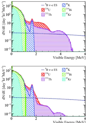
purification approaches. Three of them focus on the re-moval of natural radioactivity in LS during distillation, water extraction and gas stripping [42]. An additional on-line monitoring system (OSIRIS [43]) will be built to measure the U, Th, and Radon contaminations be-fore the LS filling. As a feasibility study, following the assumptions in the JUNO Yellow Book [22], we start with 10 g/g U and Th in the secular equilibrium, which are close to those of Borexino Phase I [44]. However, from Borexino's measurements the daughter nuclei of Rn, i.e., Pb and Po, are likely off-equi-librium. In this study g/g Pb and a Po decay rate of 2600 cpd/kt are assumed [45]. The left plot of Fig. 8 shows the internal background spectrum under the as-sumptions above, and the B neutrino signal is also drawn for comparison. Obviously, an effective back-ground reduction method is needed. The peaks are not included since after LS quenching their visible energies are usually less than 1 MeV, much smaller than the 2 MeV analysis threshold.
214 212
Above the threshold the background is dominated by five isotopes as listed in Table 2. Bi and 64% of Bi decays can be removed by the coincidence with their
γ
γ 208
Fig. 7. Deposited energy spectra in LS by external 's after different FV cuts. The plot is generated by the simulation with measured radioactivity values of all external components. The multiple 's of Tl decays in acrylic and SS nodes account for the background in 3 to 5 MeV. With a set of energy-de-pendent FV cuts, the external background is suppressed to less than 0.5% compared to signals.
8
3 − 5 208
214 212
Fig. 8. Internal radioactivity background compared with B signal before (left) and after (right) time, space and energy correlation cuts to remove the Bi-Po/Bi-Tl cascade decays. The events in the MeV energy range are dominated by Tl decays, while those between 2 and 3 MeV are from Bi and Bi.
214 τ∼ 231 µ 212 τ∼ 431 214 µ 212 212 212 212 212 212
short-lived daughter nuclei, Po ( s) and Po ( ns), respectively. The removal efficiency of Bi can reach to about 99.5% with less than 1% loss of signals. Based on the current electronics design, which records PMT waveforms in a 1 s readout window with a sampling rate of 1 G samples/s [46], it is assumed that Po cannot be identified from its parent Bi if it de-cays within 30 ns. Thus, for the Bi- Po cascade de-cays the removal efficiency is only 93%. For the residual 7%, the visible energies of Bi and Po decays are ad-ded together because they are too close to each other.
214 212 208 212 208 α 208 τ∼ 212 α 208 210 α 3 − 5
Besides removing Bi and Bi via the prompt cor-relation which was also used in previous experiments, a new analysis technique of this study is the reduction of
Tl. 36% of Bi decays to Tl by releasing an particle. The decay of Tl ( 4.4 minutes) dominates the background in the energy range of 3 to 5 MeV. With a 22 minutes veto in a spherical volume of radius 1.1 m around a Bi candidate, 99% Tl decays can be re-moved. The fraction of removed good events, estimated with the simulation, is found to be about 20%, because there are more than 2600 cpd/kt Po decays in the sim-ilar energy range. Eventually, the signal over back-ground ratio in the energy range of MeV is signific-antly improved from 0.6 to 35.
228 234 m
238 232
However, for Ac and Pa , both of which have decay energies slightly larger than 2 MeV, there are no available cascade decays for background elimination. If the U and Th decay chains are in secular equilibri-um, their contributions can be statistically subtracted with the measured Bi-Po decay rates. Otherwise the analysis threshold should be increased to about 2.3 MeV.
238 232 10−16 10−15 208 238 232 10−17 210 208 208
Considering higher radioactivity level assumptions, if the U and Th contaminations are g/g, the 2 MeV threshold is still achievable but with a worse S/B ra-tio in the energy range of 3 to 5 MeV. A g/g con-tamination would result in a 5 MeV analysis threshold de-termined by the end-point energy of Tl decay. If U and Th contaminations reach to g/g, but the Po decay rate is more than 10,000 cpt/kt as in the Borexino Phase I [44], the Tl reduction mentioned above cannot be performed. Consequently, the Tl
background could only be statistically subtracted. The in-fluence of these radioactivity level assumptions on the neutrino oscillation studies will be discussed in Sec. 4.3.
B. Cosmogenic isotopes
2
11
In addition to natural radioactivity, another crucial background comes from the decays of light isotopes pro-duced by the cosmic-ray muon spallation process in LS. The relatively shallow vertical rock overburden, about 680 m, leads to a 0.0037 Hz/m muon flux with an aver-aged energy of 209 GeV. The direct consequence is the about 3.6 Hz muons passing through the LS target. More than 10,000 C isotopes are generated per day, which constrains the analysis threshold to 2 MeV, as shown in
Fig. 9. Based on the simulation and measurements of
pre-vious experiments, it is found that other isotopes can be suppressed to a 1% level with a cylindrical veto along the muon track and the Three-Fold Coincidence cut (TFC) among the muon, the spallation neutron capture, and the isotope decay [48, 49]. Details are presented in this sec-tion.
1. Isotope generation
e± γ π± π0
γ π
When a muon passes through the LS, along with the ionization, many secondary particles are also generated, including , , , and . Neutrons and isotopes are produced primarily via the ( , n) and inelastic scatter-ing processes. More daughters could come from the neut-ron inelastic scattering on carbon. Such a process is defined as a hadronic shower in which most of the cos-mogenic neutrons and light isotopes are generated. More discussion on the muon shower process can be found in Refs. [52, 53]. To understand the shower physics and de-velop a reasonable veto strategy, a detailed muon simula-tion has been carried out. The simulasimula-tion starts with CORSIKA [54] for the cosmic air shower simulation at the JUNO site, which gives the muon energy, momentum and multiplicity distributions arriving the surface. Then MUSIC [55] is employed to track muons traversing the rock to the underground experiment hall based on the loc-al geologicloc-al map. The muon sample after transportation is used as the event generator of Geant4, with which the
238 232 214
212 208
Table 2. Isotopes in the U and Th decay chains with decay energies larger than 2 MeV. With correlation cuts most of Bi, Bi and Tl decays can be removed. The decay data are taken from Ref. [47].
Isotope Decay mode Decay energy τ Daughter Daughter's τ Removal eff. Removed signal
214Bi β− 3.27 MeV 28.7 min 214Po 237 sµ >99.5% <1%
212Bi β−: 64% 2.25 MeV 87.4 min 212Po 431 ns 93% ∼0
212Bi α: 36% 6.21 MeV 87.4 min 208Tl 4.4 min N/A N/A
208Tl β− 5.00 MeV 4.4 min 208Pb Stable 99% 20%
234Pam β− 2.27 MeV 1.7 min 234U 245500 years N/A N/A
228Ac β− 2.13 MeV 8.9 h 228Th 1.9 years N/A N/A
detector simulation is performed and all the secondary particles are recorded. A simulation data set consisting of 16 million muon events is prepared, corresponding to about 50 days statistics.
In the simulation the average muon track length in LS
is about 23 m and the average deposited energy via ioniz-ation is 4.0 GeV. Given the huge detector size, about 92% of the 3.6 Hz LS muon events consist of one muon track, 6% have two muon tracks, and the rest have more than two. Events with more than one muon track are called muon bundles. In general, muon tracks in one bundle are from the same air shower and are parallel. In more than 85% of the bundles, the distance between muon tracks is larger than 3 m. E0.74 µ Eµ γ π 11 10 11 12 γ,n 10 12 π+,np
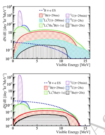
The cosmogenic isotopes affecting this analysis are listed in Table 3. The simulated isotope yields are found to be lower than those measured by KamLAND [50] and Borexino [51]. Thus, in our background estimation the yields are scaled to the results of the two experiments, by empirically modelling the production cross section as be-ing proportional to , where is the average energy of the muon at the detector. Because the mean free paths of 's, 's and neutrons are tens of centimeter in LS, the generation positions of the isotopes are close to the muon track, as shown in Fig. 10. For more than 97% of the iso-topes, the distances are less than 3 m, leading to an effect-ive cylindrical veto along the reconstructed muon track. However, the veto time could only be set to 3 to 5 s to keep a reasonable detector live time, which removes a small fraction of C and C. Thus, as mentioned before, the C, primarily from the C ( ) reaction, with the largest yield and a long life time, will push the analysis threshold of the recoil electron to 2 MeV. The removal of C, mainly generated in the C ( ) reaction, relies on the TFC among the muon, the neutron capture, and the isotope decay.
To perform the cylindrical volume veto, the muon track reconstruction is required. There have been several reconstruction algorithms developed for JUNO as repor-ted in Refs. [56–59]. A precision muon reconstruction al-gorithm was also developed in Double Chooz [60]. Based
Table 3. Summary of the cosmogenic isotopes in JUNO. The isotope yields extracted from the Geant4 simulation, as well as the ones scaled to the measurements, are listed. The TFC fraction means the probability of finding at least one spallation neutron capture event between the muon and the isotope decay.
Isotope Decay mode Decay energy (MeV) τ Yield in LS (/day) TFC fraction
Geant4 simulation Scaled
12B β− 13.4 29.1 ms 1059 2282 90% 9Li β−: 50% 13.6 257.2 ms 68 117 96% 9C β+ 16.5 182.5 ms 21 160 >99% 8Li β−+ α 16.0 1.21 s 725 649 94% 6He β− 3.5 1.16 s 526 2185 95% 8B β++ α ∼18 1.11 s 35 447 >99% 10C β+ 3.6 27.8 s 816 878 >99% 11Be β− 11.5 19.9 s 9 59 96% 11C β+ 1.98 29.4 min 11811 46065 98% 11
Fig. 9. Cosmogenic background before (left) and after veto (right). The isotope yields shown here are scaled from the KamLAND's [50] and Borexino's measurements [51]. The huge amount of C constrains the analysis threshold to 2 MeV. The others isotopes can be well suppressed with veto strategies discussed in the text.
on these studies the muon reconstruction strategy in JUNO is assumed as: 1) If there is only one muon in the event, the track could be well reconstructed. 2) If there are two muons with a distance larger than 3 m in one event, which contributes 5.5% to the total events, the two muons could be recognized and both well reconstructed. If the distance is less than 3 m (0.5%), the number of muons could be identified via the energy deposit but only one track could be reconstructed. 3) If there are more than two muons in one event (2%), it is conservatively as-sumed no track information can be extracted and the whole detector would be vetoed for 1 s. 4) If the energy deposit is larger than 100 GeV (0.1%), no matter how many muons in the event, it is assumed no track can be reconstructed from such a big shower.
To design the TFC veto, the characteristics of neut-ron production are obtained from the simulation. About 6% of single muons and 18% of muon bundles produce neutrons, and the average neutron numbers are about 11 and 15, respectively. Most of the neutrons are close to each other, forming a spherical volume concentrated with the neutrons. This volume can be used to estimate the shower position. The simulated neutron yields are com-pared with the data in several experiments, such as Daya Bay [61], KamLAND [50] and Borexino [62]. The differ-ences are found to be less than 20%. The spatial distribu-tion of the neutrons, defined as the distance between the neutron capture position and its parent muon track, are shown in Fig. 10. More than 90% of the neutrons are cap-tured within 3 m from the muon track, consistent with KamLAND's measurement. The advantage of LS detect-ors is the high detection efficiency of the neutron capture on hydrogen and carbon, which could be as high as 99%. If there is at least one neutron capture between the muon and the isotope decay, the event is defined as TFC tagged. Then the TFC fraction is the ratio of the number of tagged isotopes to the total number of generated iso-tope. In Table 3 the TFC fraction in simulation is
sum-11 10
marized. The high TFC fraction comes from two aspects: the first one is that a neutron and an isotope are simultan-eously produced, like the C and C. The other one is the coincidence between one isotope and the neutron(s) generated in the same shower. If one isotope is produced, the median of neutrons generated by this muon is 13, and for more than one isotopes, the number of neutrons in-creases to 110, since isotopes are usually generated in showers with large energy deposit. The red line in Fig. 10
shows the distance between an isotope decay and the nearest neutron capture, which is mostly less than 2 m.
2. Veto strategy
Based on the information above, the muon veto strategy is designed as below.
● Whole detector veto:
Veto 2 ms after every muon event, either passing through LS or water;
Veto 1 s for the muon events without reconstructed tracks.
● The cylindrical volume veto, depending on the dis-tance (d) between the candidate and the muon track:
d < Veto 1 m for 5 s; <d < Veto 1 m 3 m for 4 s; <d < Veto 3 m 4 m for 2 s; <d < Veto 4 m 5 m for 0.2 s. ● The TFC veto:
Veto a 2 meter spherical volume around a spallation neutron candidate for 160 s.
8 8 12 12 n, p γ π 10 11 8 8 6
In the cylindrical volume veto, the 5 s and 4 s veto time is determined based on the life of B and Li. The volume with d between 4 and 5 m is mainly to remove B, which has a larger average distance because the primary generation process is C( ) and neutrons have larger mean free path than 's and 's. For muon bundles with two muon tracks reconstructed, the above cylindric-al volume veto will be applied to each track. Compared to the veto strategies which reject any signal within a time window of 1.2 s and a 3 m cylinder along the muon track [22, 63], the above distance-dependent veto significantly improves the signal to background ratio. The TFC veto is designed for the removal of C and Be. Moreover, it effectively removes B, Li, and He generated in large showers and muon bundles without track reconstruction abilities.
The muons not passing through LS, defined as extern-al muons, will contribute to about 2% of isotopes, con-centrated at the edge of the LS. Although there is no available muon track for the background suppression, the FV cut can effectively eliminate these isotopes and reach a background over signal ratio of less than 0.1%, which can be safely neglected.
8
To estimate the dead time induced by the veto strategy and the residual background, a toy Monte Carlo sample is generated by mixing the B neutrino signal
Fig. 10. Distribution of the simulated distance between an isotope and its parent muon track (black), and the distance between the isotope and the closest spallation neutron candid-ate (red). The distance between a spallation neutron capture and its parent muon is also shown in blue.
12 8 6 10 11
e− 10 e++ γ
with the simulated muon data. The whole detector veto and the cylindrical volume veto introduce 44% dead time, while the TFC veto adds an additional 4%. The residual backgrounds above the 2 MeV analysis threshold consist of B, Li, He, C, and Be, as shown in Fig. 9. A potential improvement on the veto strategy may come from a joint likelihood based on the muon energy deposit density, the number of spallation neutrons, time and dis-tance distributions between the isotope and muon, and among the isotope and neutrons. In addition, this study could profit from the developing topological method for the discrimination between the signal ( ) and back-ground ( C, ) [56],
in situ
12 8
6 10 11
The actual isotope yields, distance distributions, and TFC fractions will be measured - in future. Estima-tion of residual backgrounds and uncertainties will rely on these measurements. Currently the systematic uncer-tainties are assumed based on KamLAND's measure-ments [40], given the comparable overburden (680 m and 1000 m): 1% uncertainty to B, 3% uncertainty to Li and He, and 10% uncertainty to C and Be.
C. Reactor antineutrinos 2 × 10⁷ 2 νe νx e+ µ ν− e 8 ν
The reactor antineutrino flux at JUNO site is about /cm /s assuming 36 GW thermal power. Combin-ing the oscillated antineutrino flux with the correspond-ing cross section [64], the Inverse Beta Decay (IBD) re-action rate between and proton is about 4 cpd/kt, and the elastic scattering rate between and electron is about 1.9 cpd/kt in the energy range of 0 to 10 MeV. The products of IBD reaction, and neutron, can be rejected to less than 0.5% using the correlation between them. The residual mainly comes from the two signals falling into one electronics readout window (1 s). The recoil elec-tron from the ES channel, with a rate of 0.14 cpd/kt when the visible energy is larger than 2 MeV, cannot be distinguished from B signals. A 2% uncertainty is as-signed to this background according to the uncertainties of antineutrino flux and the ES cross section.
IV. Expected results
After applying all the selection cuts, about 60,000
re-212 −208
12
coil electrons and 30,000 background events are expec-ted in 10 years of data taking as lisexpec-ted in Table 4 and shown in Fig. 11. The dead time due to muon veto is about 48% in the whole energy range. As listed in Table 2, the Bi Tl correlation cut removes 20% of sig-nals in the energy range of 3 to 5 MeV, and less than 2% in other energy ranges. The detection efficiency uncer-tainty, mainly from the FV cuts, is assumed to be 1% ac-cording to Borexino's results[23]. Given that the uncer-tainty of the FV is determined using the uniformly dis-tributed cosmogenic isotopes, the uncertainty is assumed to be correlated among the three energy-dependent FVs. Since a spectrum distortion test will be performed, anoth-er important uncanoth-ertainty source is the detector enanoth-ergy scale. For electrons with energies larger than 2 MeV, the nonlinear relationship between the LS light output and the deposited energy is less than 1%. Moreover, elec-trons from the cosmogenic B decays, with an average energy of 6.4 MeV, can set strong constraints to the en-ergy scale, as it was done in Daya Bay [35] and Double Chooz [65]. Thus, a 0.3% energy scale uncertainty is used in this analysis following the results in Ref. [35]. Three analyses are reported based on these inputs.
∆m2⋆
21 4.8 × 10⁻⁵ 2 ∆m2†21 7.5 × 10⁻⁵ 2
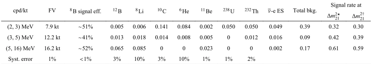
Table 4. Summary of signal and background rates in different visible energy ranges with all selection cuts and muon veto methods applied. = eV , and = eV
cpd/kt FV 8B signal eff. 12B 8Li 10C 6He 11Be 238U 232Th ν-e ES Total bkg. Signal rate at ∆m2⋆ 21 ∆m2†21 (2, 3) MeV 7.9 kt ∼51% 0.005 0.006 0.141 0.084 0.002 0.050 0.050 0.049 0.39 0.32 0.30 (3, 5) MeV 12.2 kt ∼41% 0.013 0.018 0.014 0.008 0.005 0 0.012 0.016 0.09 0.42 0.39 (5, 16) MeV 16.2 kt ∼52% 0.065 0.085 0 0 0.023 0 0 0.002 0.17 0.61 0.59 Syst. error 1% <1% 3% 10% 3% 10% 1% 1% 2% ∆m2 21 4.8 × 10⁻⁵ 2
Fig. 11. Expected signal and background spectra in ten years of data taking, with all selection cuts and muon veto methods applied. Signals are produced in the standard LMA-MSW framework using = eV . The energy dependent fiducial volumes account for the discontinuities at 3 MeV and 5 MeV.
A. Spectrum distortion test νµ,τ Pee ∆m221 4.8 × 10⁻⁵ 2 νe ×106 2 ∆m221 7.5 × 10⁻⁵ 2 ∆m221
In the observed spectrum, the upturn comes from two aspects: the presence of , and the upturn in . A background-subtracted Asimov data set is produced in the standard LMA-MSW framework using =
eV , shown as the black points in the top panel of Fig. 12. The other oscillation parameters are taken from PDG 2018 [33]. The error bars show only the statistical uncer-tainties. The ratio to the prediction of no-oscillation is shown as the black points in the bottom panel of Fig. 12. Here no-oscillation is defined as pure with an arrival flux of 5.25 /cm /s. The signal rate variation with re-spect to the solar zenith angle has been averaged. The ex-pected signal spectrum using = eV is also drawn as the red line for comparison. More signals can be found at the low energy range. The spectral differ-ence provides the sensitivity that enables measurement of
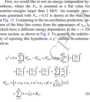
. Pee Pee=0.32 νµ,τ ν− e χ2
First, we would like to test an energy-independent hy-pothesis, where the is assumed as a flat value for neutrino energies larger than 2 MeV. An example spec-trum generated with is drawn as the blue line
in Fig. 12. Comparing to the no-oscillation prediction,
up-turn of the blue line comes from the appearance of 's, which have a different energy dependence in the ES cross section, as shown in Fig. 4. To quantify the sensitiv-ity of rejecting this hypothesis, a statistic is construc-ted as: χ2=2 × 140 ) i=1 ⎛ ⎜⎜⎜⎜⎝Ni
pre− Nobsi +Nobsi × log Ni obs Ni pre ⎞ ⎟⎟⎟⎟⎠+$εd σd %2 + $ε f σf %2 + $ εs σs %2 + $ εe σe %2 + 10 ) j=1 ⎛ ⎜⎜⎜⎜⎜ ⎝ εbj σbj ⎞ ⎟⎟⎟⎟⎟ ⎠ 2 , Nipre= 0 1 + εd+ εf+ αi× εs+ βi×0.3%εe 1 × Ti + 10 ) j=1 (1 + εbj) × Bi j, (2) Ni obs ith
where is the observed number of events in the
en-Ni pre Ti Pee Bi j σd σf σbj jth εd εf εbj
ergy bin in the LMA-MSW framework, is the pre-dicted one in this energy bin, by adding the signal gen-erated under the flat hypothesis with the back-grounds , which is summing over j. Systematic uncer-tainties are summarized in Table 5. The detection effi-ciency uncertainty is (1%), the neutrino flux uncer-tainty is (3.8%), and is the uncertainty of the background summarized in Table 4. The corresponding nuisance parameters are , , and , respectively.
8 ν σs σe αi βi σ αi εs βi
The two uncertainties relating to the spectrum shape, the B spectrum shape uncertainty and the detector energy scale uncertainty , are implemented in the stat-istic using coefficients and , respectively. The neut-rino energy spectrum with 1 deviation is converted to the visible spectrum of the recoil electron. Its ratio to the visible spectrum converted from the nominal neutrino spectrum is denoted as . In this way, the corresponding nuisance parameter, , follows the standard Gaussian distribution. For the 0.3% energy scale uncertainty, is derived from the ratio of the electron visible spectrum
8 ν αi σs
Table 5. Summary of the systematic uncertainties. Since the uncertainty of B spectrum shape is absorbed in the coefficients , equals to 1. See text for details.
Notation Value Reference
Detection efficiency σd 1% Borexino [23]
Detector energy scale σe 0.3% Daya Bay [35], Double Chooz [65]
8 ν
The B flux σf 3.8% SNO [25]
8 ν
The B spectrum shape σs 1 Ref. [26]
jth
The background σbj Table 4 This study
∆m2 21
Pee=0.32(Eν>2 MeV)
Fig. 12. Background subtracted spectra produced in the standard LMA-MSW framework for two values (black dots and red line, respectively), and the
assumption (blue line). Their comparison with the no flavor conversion is shown in the bottom panel. Only statistical un-certainties are drawn. Details can be found in the text.
shifted by 0.3% to the visible spectrum without shifting. χ2 Pee(Eν>2 MeV) ∆χ2 σf Pee ∆m2 21 ∆m221 7.5 × 10⁻⁵ 2 σ Pee ∆χ2=4.9 ∆m2 21=4.8 × 10⁻⁵ 2 7.5 × 10⁻⁵ 2 ∆χ2=7.1
By minimizing the , the abilities of excluding the flat hypothesis, in terms of values, are listed in Table 6. The total neutrino flux is con-strained with a 3.8% uncertainty ( ) from the SNO NC measurement, while the value is free in the minimiza-tion. The sensitivity is higher at larger values due to the larger upturn in the visible energy spectrum. If the true value is eV , the hypothesis could be rejected at 2.7 level. The statistics-only sensitivity of re-jecting the flat hypothesis is (18.9) for eV ( eV ) for 3 MeV threshold, comparing to (24.9) for 2 MeV threshold.
∆m221 7.5 × 10⁻⁵ 2
σs
σe
To understand the effect of systematics, the impact of each systematic uncertainty is also provided in Table 6. The sensitivity is significantly reduced after introducing the systematics. For instance, with =
eV , including the neutrino spectrum shape uncertainty ( ) almost halved the sensitivity, because the shape un-certainty could affect the ratio of events in the high and low visible energy ranges. If the detector energy scale un-certainty ( ) is included, the sensitivity is also signific-antly reduced due to the same reason above.
B. Day-Night asymmetry ∆m2 21 ∆m2 21 4.8 × 10⁻⁵ 2 7.5 × 10⁻⁵ 2 ∆m2 21
Solar neutrino propagation through the Earth is ex-pected, via the MSW effect, to cause signal rate variation versus the solar zenith angle. This rate variation observ-able also provides additional sensitivity to the value, as shown in Fig. 13. The blue and red dashed lines represent the average ratio of the measured signal to the no-oscillation prediction, and they are calculated with = eV and eV , respectively. The solid lines show the signal rate variations versus sol-ar zenith angle. Smaller values result in a larger MSW effect in the Earth and increased Day-Night asym-metry. The error bars are the expected uncertainties.
The variation is quantified by defining the Day-Night asymmetry as: ADN= RD− RN (RD+RN)/2, (3) RD RN cosθz<0 cosθz>0 σ ∆m221 4.8 × 10⁻⁵ 2 10 σ ∆m221 7.5 × 10⁻⁵ 2 A DN (−1.6 ± 0.9) ADN ∆m2 21
where and are the background-subtracted signal rates during the Day ( ) and Night ( ), re-spectively. They are obtained by dividing the signal num-bers listed in Table 7 by the effective exposure in Fig. 2. The uncertainties are propagated with a toy Monte Carlo program to correctly include the correlation among sys-tematics. With ten years data taking, JUNO has the poten-tial to observe the Day-Night asymmetry at a signific-ance of 3 if = eV . Even when restrict-ing to an energy range from 5 to 16 MeV, within which neither natural radioactivity nor C are significant, a 2.8 significance can still be achieved. If = eV , the expected is for the 2 to 16 MeV energy range. The different values also contribute to the determination.
ADN
The measurement uncertainty is dominated by
Pee(Eν>2 MeV) ∆m2
21
Table 6. Rejection sensitivity for the flat hy-pothesis with 10 years data taking for the two values. The impact of each systematic uncertainty is also listed separ-ately.
∆χ2 4.8 × 10⁻⁵ eV2 7.5 × 10⁻⁵ eV2
Stat. only 7.1 24.9
8
Stat. + B flux error 6.8 24.2
8
Stat. + B shape error 3.6 11.8
Stat. + energy scale error 4.7 15.5
Stat. + background error 3.6 14.0
Final 2.0 7.3
∆m2 21 4.8 × 10⁻⁵ 2
Table 7. Number of the background-subtracted signals dur-ing Day and Night in ten years of data takdur-ing for = eV . A set of energy-dependent FV cuts are used and the values of the three energy ranges are provided. The uncertainties are dominated by signal and background statist-ics.
Energy Exposure Day Night ADN
∼ 2 3 MeV 41 kt y· 4334 4428 (-2.1 3.2)%± ∼ 3 5 MeV 51 kt y· 8686 8906 (-2.5 1.7)%± ∼ 5 16 MeV 84 kt y· 17058 17644 (-3.4 1.2)%± ∼ 2 16 MeV N/A 30078 30977 (-2.9 0.9)%± 8
Fig. 13. Ratio of B neutrino signals produced in the stand-ard LMA-MSW framework to the no-oscillation prediction at different solar zenith angles. The uncertainties are propagated with a toy Monte Carlo simulation, and most of the systemat-ic uncertainties are cancelled.