Corso di Perfezionamento in Fisica
Critical Behavior of Systems with
Complex Symmetries
Supervisor
Candidate
Prof. Ettore Vicari
Pasquale Calabrese
Contents
Introduction
1
1 Multicoupling Landau Ginzburg Wilson Hamiltonian
3
1.1 Mean-Field Theory . . . .
4
1.2 RG approach . . . .
5
1.3 The field-theoretical approach to LGW Hamiltonians with a single quadratic
invariant . . . .
5
1.3.1
The fixed-dimension expansion . . . .
6
1.3.2
The ² expansion . . . .
8
1.3.3
The MS scheme without ² expansion . . . .
9
1.3.4
The pseudo-² expansion . . . 10
1.4 The Analysis of perturbative series . . . 10
1.4.1
Large order behavior . . . 11
1.4.2
Resummation of the perturbative series . . . 15
1.5 Other Field-Theoretical Methods . . . 16
1.5.1
The 1/N expansion . . . 16
1.5.2
The non-linear σ model and d − 2 expansion . . . 18
1.5.3
The so-called exact RG . . . 19
1.6 Lattice techniques . . . 20
1.6.1
Monte Carlo simulations . . . 20
1.6.2
High Temperature expansion . . . 21
2 O(N ) Models
23
2.1 Overview . . . 23
2.2 Stability of the three-dimensional O(N ) fixed point . . . 26
2.2.1
Comparison with experiments . . . 28
3 Critical crossover
29
3.1 Crossover in φ
4theories . . . 31
3.2 Crossover behavior in multicoupling systems . . . 32
3.2.1
RG trajectories . . . 33
3.2.2
Crossover functions in multicoupling Hamiltonians . . . 34
3.3 Universal Ratios of scaling correction amplitudes . . . 34
4 The Cubic and the M N Models
37
4.1 Three-Dimensional Results . . . 40
4.1.1
RG dimensions of bilinear operators in the cubic-symmetric theory . . . 42
4.2 The Three-Dimensional M N model . . . 43
iii
4.2.2
Fixed points from resummation of perturbative series. . . 45
4.2.3
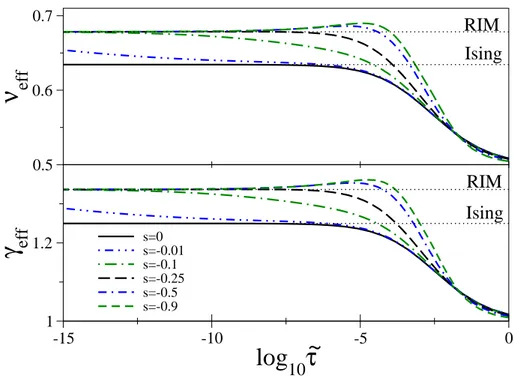
Crossover behavior and effective exponents. . . 47
4.3 The two dimensional cubic model . . . 48
4.3.1
Field-Theoretical Results . . . 48
4.3.2
The M N model for N, M ≥ 2 . . . 53
5 Random Systems
55
5.1 The Harris Criterion . . . 56
5.2 The Randomly Dilute Ising Model . . . 57
5.2.1
Field-theoretical approach: an overview . . . 57
5.2.2
Re-analysis of MZM series . . . 59
5.3 Random O(M ) model . . . 60
5.4 Crossover in three-dimensional dilute spin systems . . . 61
5.4.1
RG trajectories for dilute spin systems . . . 62
5.4.2
Crossover from Gaussian to random critical behavior in Ising systems . 63
5.4.3
Crossover from Ising to random critical behavior . . . 64
5.4.4
Crossover in randomly dilute multicomponent spin systems . . . 68
5.4.5
Universal ratios of scaling correction amplitudes for dilute spin systems
69
5.5 Random impurities and softening: General considerations . . . 71
5.6 Randomly Dilute Spin Models with Cubic Symmetry . . . 72
5.6.1
General considerations on the RG flow . . . 73
5.6.2
The RG flow near four dimensions . . . 74
5.6.3
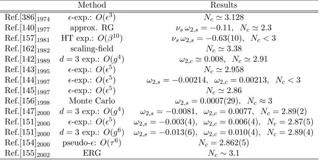
Analysis of the six-loop fixed-dimension expansion. . . 74
5.7 The Random Field Ising Model . . . 76
5.7.1
Crossover from random exchange to random field critical behavior in
Ising models . . . 76
6 Spin models with random anisotropy and reflection symmetry
79
6.1 Effective Φ
4Hamiltonians . . . 81
6.2 General renormalization-group properties . . . 83
6.2.1
Fixed points of the theory . . . 83
6.2.2
Crossover behavior close to the pure spin model . . . 84
6.2.3
Stable fixed points . . . 86
6.2.4
Critical behavior for infinitely strong random anisotropy . . . 87
6.3 Renormalization-group flow in the quartic-coupling space . . . 88
6.3.1
Results . . . 88
7 3D Frustrated Models with non-collinear order
91
7.1 LGW Hamiltonian . . . 92
7.2 Experimental results and Monte Carlo simulations . . . 93
7.3 A brief overview of FT results . . . 95
7.3.1
Mean-Field approximation . . . 95
7.3.2
² expansion . . . 96
7.3.3
Other FT investigations . . . 97
7.4 Five-loop ² expansion results . . . 99
7.4.1
Critical exponents . . . 102
7.5 Six-loop pseudo-² results for n
±(m, 3) . . . 103
7.6 Limits of the ² expansion and other methods predicting a first-order transition 105
iv
7.7.1
The-six loop RG functions . . . 105
7.7.2
Focus-like behavior at the chiral fixed point for physical values of n . . 106
7.7.3
Crossover behavior: effective exponents . . . 108
7.7.4
Results for n > 3 . . . 110
7.8 Five-loop MS scheme without ²-expansion . . . 113
7.9 The “collinear” region v
0< 0 . . . 117
7.9.1
Exact analysis for n = 2 . . . 118
7.9.2
Five-loop ²-expansion and six-loop pseudo-² . . . 118
7.9.3
Resummation of MZM and MS β functions for n = 3 . . . 119
7.9.4
n > 3 in the collinear region . . . 120
7.10 RG dimensions of the quadratic perturbations . . . 120
7.11 A Monte Carlo simulation of the LGW Hamiltonian . . . 122
7.11.1 The phase diagram for A
22> A
4= 1 . . . 123
7.11.2 A model with a continuous transition: A
22= 7/5 . . . 124
7.12 Conclusions . . . 124
8 2D Frustrated Models with non-collinear order
127
8.1 Experimental results and Monte Carlo simulation . . . 128
8.2 Field-Theory analysis in fixed dimension d = 2 . . . 129
8.2.1
The analysis method . . . 129
8.2.2
Large n analysis (n ≥ 4) . . . 130
8.2.3
Physical n . . . 132
8.2.4
Renormalization-group flow and crossover . . . 133
8.3 Conclusions . . . 133
9 Multicritical phenomena in O(n
1)⊕O(n
2)-symmetric theories
135
9.1 RG flow at the multicritical point . . . 137
9.2 Discussions . . . 139
10 Multicritical behavior in frustrated spin systems with noncollinear order 143
10.1 Derivation of the Φ
4Hamiltonian and mean-field analysis . . . 145
10.1.1 Mean-field phase diagram . . . 147
10.2 Particular models and fixed points . . . 150
10.2.1 Stability of the O(2)⊗O(N ) fixed points . . . 152
10.2.2 Stability of the decoupled [O(2)⊗O(N − 1)]⊕O(2) fixed points . . . 153
10.3 The renormalization-group flow in the full theory . . . 154
10.3.1 Renormalization-group flow near four dimensions . . . 154
10.3.2 RG flow in the 3d-MS scheme for N = 3 . . . 155
10.4 Conclusions . . . 155
11 U (n) × U (m) models and finite-temperature phase transition in QCD
157
11.1 Five-loop ²-expansion of U (n) × U (m) model. . . 159
11.1.1 Estimates of n
+(m, 3) . . . 159
11.2 Pseudo-² expansion . . . 160
11.3 The effect of the anomaly . . . 161
11.4 Conclusions . . . 162
Bibliography
165
Introduction
A phase transition is defined as a singularity in thermodynamic quantities of a system. Phase
transitions are classified, according to Ehrenfest, as first order, second order . . . , or first
order and continuous. The starting point of the classification is the rigorous result that
the free energy is always a continuous function (e.g. in the grancanonical ensemble) of the
temperature and chemical potential. But it may be nonanalytic. If one of its first derivatives
is discontinuous (internal energy, magnetization, volume, . . . ) the transition is first order; if
one of the second derivatives (specific heat, susceptibility, . . . ) is discontinuous the transition
is second order, and so on. Defining via singularities is the most general way of characterizing
a phase transition. For a large class of systems, singularities could occur due to ordering
after a phase transition (symmetry breaking), but this is not necessarily a requirement for
all transitions. In other words, the existence of an order parameter is not a prerequisite for
understanding phase transitions though it might be very useful in many contexts.
The behavior of a system close to a continuous phase transition is distinctly different from
the behavior far from it. This difference is so important that we refer to a continuous phase
transition as a critical phenomenon. Power laws are distinctive features of critical phenomena
and can be ascribed to diverging length-scale. This connection is now so well-characterized
that any phenomena, equilibrium or not equilibrium, thermal or non thermal, showing power
laws tend to be interpreted in the same manner as equilibrium critical phenomena through
the identification of relevant terms, scaling and diverging lengths. The exponents describing
the rate of divergence of physical quantities are named critical exponents and their proper
determination has been attracting generations of physicists in the last thirty years. Nowadays
there is a special dictionary for these exponents. For instance, in the case of a thermal
phase transition, whose driving parameter is the temperature, the exponent of specific heat
is α (C = A
±|t|
α, where t = T − T
c), the one of magnetization (using the common magnetic
language) in the ordered phase β (M ∝ (−t)
β), γ for the susceptibility χ = ∂M/∂h|
h=0∝ t
−γ.
The behavior of the diverging scaling-length at the critical point is fundamental, and it is
described by the exponent ν, i.e. ξ ∝ |t|
−ν. At the critical point the correlation length
diverges and the two point function has a power law behavior governed by the exponent η:
hM (x)M (0)i = |x|
2−d−η.
One of the most important contribution to the understanding of the critical phenomena
was the introduction of Renormalization Group (RG) ideas, which allowed the shift in point of
view to a classification of the terms of a Hamiltonian as relevant or irrelevant, rather than refer
to them as numerically weak or strong. It is not my aim here to give a complete overview of a
so long and complicated task, in this Introduction I only want to fix few general ideas behind
RG and I remand for an exhausting treatment to the textbooks quoted in the bibliography.
Close to the critical point the only important length scale is the correlation length, which
diverges at the critical point, leaving the system without a length scale, i.e. scale invariant.
Let us consider explicitly an Hamiltonian system. The “appropriate scale transformation”,
called RG transformation, is a mapping in the abstract space of Hamiltonians H
−→ H
G 0(on
a practical model this transformation may be done in several way, e.g. by a block
trans-formation in real space, by an integration on the fast modes in momentum space . . . ). In
particular the scale invariant Hamiltonians are those that do not change under this
transfor-mation GH
∗= H
∗. Close to these fixed points the RG transformation may be linearized,
leading to a linear operator L which possess an (infinite) number of eigenvalues y
iand (left or
right) eigenoperators O
i. A general Hamiltonian, close to the fixed point, may be expanded
as (l is a scale parameter)
H = H
∗+
X
µ
iO
i,
where µ
isatisfy
dµ
idl
= y
iµ
i.
If y
ihas a positive real part the (even small) perturbation µ
igrows up and the flow goes far
from the fixed point. Such terms are called relevant. If instead y
ihas a negative real part,
the perturbation decays with the iteration of RG transformations and finally the flow reaches
the fixed point. These operator are called irrelevant. If y
i= 0 the operator is called marginal
and the fate of the Hamiltonian will depend on the higher order terms in the RG equations.
From these abstract RG equations a fundamental feature of critical phenomena emerges:
Universality. Independently from the Hamiltonian (and, even more, independently from what
it describes), all the systems in the domain of attraction of a certain H
∗have the same critical
behavior. Usually at a thermal phase transition, one has to tune only two relevant
parame-ters to reach the critical point: the temperature to T
cand the magnetic field h to 0 (more
generally for nonmagnetic systems h is the variable conjugated to the order parameter). Thus
we can divide all the critical phenomena in a relative small number of universality classes,
characterized by the dimensions of the space, the symmetry of the system (that reduces the
number of operators one may consider), and the range of interactions.
Finally predictions may be given writing the flow equation for the free energy. Close to a
fixed point the singular part of free-energy is
F
s(h, t, . . . µ
i. . . ) ∝ |t|
d/ytF
µ
h
|t|
yh/yt, . . . ,
µ
i|t|
yi/yt
,
from which we can derive the standard exponents
α = 2 − d/y
t,
β = (1 − y
h)d/y
t,
γ = −(1 − 2y
h)d/y
t,
ν = 1/y
t,
η = d + 2 − 2dy
h.
Thus the knowledge of RG eigenvalues leads to the critical exponents. From these relations
follow the well-known scaling laws
α + 2β + γ = 2 ,
γ = ν(2 − η) ,
dν = 2 − α .
The aim of this thesis is the characterization of some universality classes having rather
complicated symmetries and describing phase transitions in models with anisotropies,
ran-domness, frustration and competing order parameters. To obtain qualitative and quantitative
predictions we calculated and analyzed higher order perturbative expansions up to six or five
loops.
Multicoupling Landau Ginzburg
Wilson Hamiltonian
In this introductory chapter we define the main subject of this thesis: The
Mul-ticoupling Landau-Ginzburg-Wilson Hamiltonians. In particular we will
empha-size on how perturbative field-theoretical methods, in conjunction with refined
resummation techniques, allow one to obtain very precise theoretical predictions
for universal quantities close to a continuous phase transition. We introduce the
perturbative approach in fixed dimension and the minimal subtraction
renormal-ization scheme with and without ² expansion. The application of these techniques
to systems with complex symmetries will be the main goal of this thesis. We end
the chapter with an overview of alternative theoretical methods to describe the
critical point, with which the perturbative methods must be confronted before of
the comparison with experiments.
A statistical model describing a second order phase transition is usually defined by a lattice
short-range Hamiltonian involving finite length spins. Typical examples are the O(N ) models
H = −
X
hiji
J
ij~s
i· ~s
j,
(1.1)
where the sum is over next-neighbor and ~s
iare N -component spin of unit length at the lattice
site i. We can replace fixed length spins with variable of unconstrained length ~
φ
iby means of
a Hubbard-Stratonovich (HS) transformation
1. Universality suggests that microscopic details
are not essential, so we can take the formal limit of zero lattice spacing, arriving to an
Hamil-tonian depending on an N -component field φ
i(x) (now i labels the components). Expanding
in power of φ
ione obtains a very complex object containing (at least in principle) all the
powers of the field, all the nth derivatives, and the products of all of them. Such Hamiltonian
is intractable. Fortunately not all these terms are relevant in the RG sense. Indeed by power
counting, one realizes that close to four dimensions the relevant terms in the Hamiltonian,
called Landau-Ginzburg-Wilson (LGW), are only the powers of the field up to the fourth
or-der (φ
4terms) and the kinetic term (∂
µ
φ
i)(∂
νφ
j). The φ
4terms of the Hamiltonian may be
1The HS transformation for a general spin model on an arbitrary lattice is the Gaussian integralePijPαβKαβij sαisβj ∝ Z dφαie 1 4 P ijPαβφαi(K−1)αβij φβj+ P i,αφαisαi .
After this transformation, the spin variables decouple and it is straightforward to sum over them, ending in an effective Hamiltonian for unconstrained modes φα
derived by the mapping into the lattice Hamiltonian. But this is not always needed. In fact
one can guess them requiring the most general form compatible with the symmetries of the
lattice Hamiltonian.
For an N -component order parameter φ
i(x), the most general LGW Hamiltonian can be
written as
H =
Z
d
dx
h 1
2
X
i(∂
µφ
i(x))
2+
1
2
X
ijr
ijφ
i(x)φ
j(x) +
4!
1
X
ijklu
ijklφ
i(x)φ
j(x)φ
k(x)φ
l(x)
i
, (1.2)
where the number of independent parameters r
ijand u
ijkldepends on the symmetry group
of the theory. Let us consider the O(N )-symmetric Hamiltonian, the introduced parameters
must have the form
u
abcd=
g
3
(δ
abδ
cd+ δ
acδ
bd+ δ
adδ
bc) ,
r
ij= δ
ijr
0.
(1.3)
Similarly, if we restrict the symmetry to the cubic one (given by the reflections and
permuta-tions of the field components) we have
u
abcd=
g
3
(δ
abδ
cd+ δ
acδ
bd+ δ
adδ
bc) + vδ
abδ
cdδ
ad,
r
ij= δ
ijr
0.
(1.4)
An interesting class of models is characterized by the fact that
P
iφ
2i
is the only quadratic
polynomial that is invariant under the symmetry group of the theory. In this case, r
ijis a
multiple of the identity, i.e. r
ij= δ
ijr
0. Moreover, u
ijklmust satisfy the trace condition
X
i
u
iikl∝ δ
kl,
(1.5)
in order to ensure that additional quadratic invariants are not generated by the RG
transfor-mations [61]. In these models, criticality is driven by tuning the single parameter r
0, which in
a thermal phase transition corresponds to the temperature, i.e. r
0= T − T
c.
As clear from above, in the absence of a sufficiently large symmetry restricting the form
of the potential, many quartic couplings must be introduced and the study of the critical
behavior may become quite complicated.
1.1
Mean-Field Theory
A first simplified analysis that leads to a qualitative description of the phase diagram of
the models described by Eq. (1.2) is given by mean-field theory. In this approximation one
neglects fluctuations of the order parameter and considers it as uniform in the space and equal
to its mean value φ
i(x) = hφ
ii. The ground-state is the configuration that minimizes H. To
make solvable this minimum problem, the Hamiltonian must be bounded, which corresponds
to the fact that the “coupling matrix” u
ijklis positive (in the sense that u
ijklv
iv
jv
kv
lis always
positive for a generic choice of the v
i’s). Assuming the positivity of u
ijkland r
ij= r
0δ
ij, we
have that for r
0≥ 0 the quartic form is minimized by hφ
ii = 0. For r
0< 0 several degenerate
minima appear. These satisfy the equations
r
0hφ
ii +
1
3!
u
ijklhφ
jihφ
kihφ
li = 0
with i = 1, . . . , N .
(1.6)
The solution is given by hφ
ii = h|φ|iv
i, where v
iare unit vectors that minimize u
ijklv
iv
jv
kv
l.
In terms of these vectors the mean-field solution for r
0< 0 is
hφi
2= −
6r
0The vanishing of the order parameter with r
0→ 0, implies a second order phase transition with
β = 1/2. Calculating other thermodynamic quantities, one obtains the mean-field (sometimes
called classical) critical exponents ν = 1/2, η = 0, and γ = 1.
Note that when u
ijklis not positive, Eq. (1.7) does not make sense. This is connected with
the fact that the Hamiltonian is not bounded. In such case we are not allowed to drop higher
order terms in φ in the LGW Hamiltonian, since they are responsible of the stability. Taking
into account these higher order contributions the transition is altered. The more relevant
term to be added is φ
6. Let us consider for simplicity the one-component case, the mean-field
Hamiltonian is
H =
1
2
r
0φ
2+
1
4!
uφ
4+
1
6!
gφ
6,
(1.8)
where we assume g > 0 (elsewhere we continue in the expansion in powers of φ until we find a
positive term). When r
0> 0, hφi = 0 is a minimum, but it is not always the lower one. The
result is a first order transition (a part from some special values of the couplings leading to a
tricritical transition).
1.2
RG approach
The mean-field theory gives exact values for the various critical exponents in a large enough
number of spatial dimensions, but it generally fails sufficiently close to the critical point in
physical dimensions, where the effect of fluctuations is important. The Ginzburg criterion leads
to the conclusion that for φ
4models, fluctuations are important in less than four dimensions
US
G
H
S
v
u
Figure 1.1:
A possible RG flow for a theory with two couplings u and v .1.3.1
The fixed-dimension expansion
In the fixed-dimension expansion one works directly in d = 3 or d = 2. In this case the theory
is super-renormalizable since the number of primitively divergent diagrams is finite (three in
three dimensions and only one in two dimensions). One may regularize the corresponding
integrals by keeping d arbitrary and performing an expansion in ² = 3 − d or ² = 2 − d. Poles
in ² appear in divergent diagrams. Such divergences are related to the necessity of performing
a renormalization of the parameter r
0appearing in the bare Hamiltonian. This problem can
be avoided by replacing r with the mass m defined by
m
−2=
1
Γ
(2)(0)
∂Γ
(2)(p
2)
∂p
2¯
¯
¯
¯
¯
p2=0,
(1.9)
where the function Γ
(2)(p
2) is related to the one-particle irreducible two-point function by
where Γ
(1,2)is the one-particle irreducible two-point function with an insertion of 1/2
P
iφ
2i.
Since the renormalization is performed on zero-momentum correlation functions in the massive
theory, we will refer to this approach as Massive Zero-Momentum (MZM) scheme. From the
perturbative expansions of the correlation functions Γ
(2), Γ
(4), and Γ
(1,2), one derives the
expansion of the RG functions we are going to define.
The FP’s of the theory are given by the common zeros g
∗abcdof the β-functions
β
ijkl(g
abcd) = m
∂g
∂m
ijkl¯
¯
¯
¯
uabcd.
(1.14)
In the case of a continuous transition, when m → 0, the couplings g
ijklare driven toward an
infrared-stable zero g
∗ijkl
of the β-functions. The stability properties of the FP’s are controlled
by the eigenvalues ω
iof the matrix
Ω
ijkl,abcd=
∂β
ijkl∂g
abcd(1.15)
computed at the given FP: a FP is stable if all eigenvalues ω
iare positive. The smallest
eigenvalue ω determines the leading scaling corrections, which vanish as m
ω∼ |t|
∆where
∆ = νω. Usually ω is associated with the leading irrelevant operator. If ω
iis negative,
∆
i= νω
iis the crossover exponents which quantifies how the RG flow goes away from the
unstable FP (see section 3). If a stable FP has ω with a non-vanishing imaginary part, it is
called focus because the approach to the FP is spiral-like.
The critical exponents are obtained by evaluating the RG functions
η
φ(g
ijkl) =
∂ ln Z
φ∂ ln m
¯
¯
¯
¯
u= β
abcd∂ ln Z
φ∂g
abcd,
η
t(g
ijkl) =
∂ ln Z
t∂ ln m
¯
¯
¯
¯
u= β
abcd∂ ln Z
∂g
t abcd(1.16)
at the stable FP g
∗ ijkl:
η = η
φ(g
ijkl∗),
ν = [2 − η
φ(g
ijkl∗) + η
t(g
ijkl∗)]
−1.
(1.17)
All the other standard exponents can be obtained using the scaling and hyperscaling relations
reported in the Introduction.
To obtain the critical exponents of the correlation functions of a generic operator O, one
introduces the new renormalization constant Z
Oof the operator O via the natural relation
Γ
(2)O(0) = Z
O−1(g
abcd)C
ijO,
(1.18)
where Γ
(2)O(0) is the zero-momentum two-point function with one insertion of the operator O,
and C
Oij
is the tensorial structure of Γ
(2)O
(0) at tree-level (e.g. for O = 1/2φ
2, C
ijO= δ
ij). The
anomalous dimension of O is given by
η
O(g
ijkl) =
∂ ln Z
O∂ ln m
¯
¯
¯
¯
u= β
abcd∂ ln Z
O∂g
abcd,
(1.19)
calculated at the stable FP. The thermodynamics of the operator O defines a new set of critical
exponents given by
hOi = (−t)
−βO,
for t < 0 ,
(1.20)
χ
O=
Z
d
dxhO(x)O(0)i
c∝ t
−γO,
(1.21)
F
sing(t, h
O) = |t|
dνF (h
O|t|
−φO) ,
(1.22)
where h
Ois the field conjugated to O, φ
O= y
Oν, and y
Ois the RG dimension of O (i.e.,
y
O= 2 + η
O− η). These exponents satisfy the scaling relations
β
O= dν − φ
O,
γ
O= −dν + 2φ
O,
β
O+ γ
O= φ
O.
(1.23)
We have computed the perturbative expansion of the correlation functions Eqs. (1.11),
(1.12), and (1.13) for several interesting LGW Hamiltonians up to six loops in three dimensions
and five loop in two dimensions. The diagrams contributing to the two-point and four-point
functions to six-loop order are reported in Ref. [44]: they are 789 for the four-point function and
88 for the two-point one (at five-loop they are 162 and 26 respectively). We have developed a
symbolic manipulation program which generates the diagrams using the algorithm described
in Ref. [43], and computes the symmetry and group factors of each of them. We did not
calculate the integrals associated to each diagram, but we used the numerical results compiled
in Ref. [44] for three dimensions and in Ref. [46] for two dimensions.
Technical remark
In fixed dimension expansion the β functions have the form
β
gi4 − d
= −g
i+ A
dC
Ng
2
i
+ O(g
j2, g
i3, g
ig
j) ∀j 6= i,
(1.24)
where A
dis the value of the single one-loop Feynman integral for the four-point function
A
d=
Γ(2 − d/2)
(4π)
d/2,
and C
Nthe combinatorial factor of the same diagram, depending only on the symmetry of
the theory. In order to have a FP value of the order of unity for all N , the change of variable
¯
g
i= A
dC
Ng
i⇒ β
g¯i= A
dC
Nβ
gi(g
i(¯
g
i))
(1.25)
is performed. After this change the β functions are
β
¯gi4 − d
= −¯
g
i+ ¯
g
2
i
+ O(¯
g
j2, ¯
g
i3, ¯
g
ig
¯
j) ∀j 6= i .
1.3.2
The ² expansion
A useful tool that allows to find the FP’s of the RG flow and permits analytical manipulations
of the results is the so called ² expansion. It is based on the observation that d = 4 is a special
dimension for φ
4LGW Hamiltonians (it is the upper critical dimension, i.e. the dimension
above which the critical behavior is mean-field like). Indeed, using the definition of the β
functions we get
β
gi({g}) = m
∂g
i∂m
¯
¯
¯
¯
0= −(4 − d)
µ
d log g
iZ
gidg
i
−1,
(1.26)
where the subscript 0 stands for derivative at fixed bare couplings. Being Z
gi= 1 + O({g}),
the fixed point g
∗i
= 0 is IR stable for d > 4 and unstable in the opposite case. Thus, for
d > 4 the critical behavior is governed by the FP g
∗i
= 0 (Gaussian FP), corresponding to
dimension from four, the new IR stable fixed point is expected to be close to the Gaussian
one, i.e., g
∗= O(²), where ² ≡ 4 − d. As originally pointed out in a seminal paper by Wilson
and Fisher [37], one can perform a double expansion of RG functions in terms of g and ² and
find the zeros of the β functions as series in ². The critical exponents and other universal
quantities are obtained expanding in ² the corresponding RG functions evaluated at the stable
fixed point.
This procedure allows to obtain the critical quantities as series in ². The analytical
contin-uation of such series at physical dimensions d = 3, 2 (i.e., ² = 1, 2) may not seem
straightfor-ward. However, the validity of this continuation to ² = 1, 2 is corroborated by the very good
agreement of the ²-expansion estimates with other theoretical and experimental values, as we
will discuss later on.
Practically, one first determines the expansion of the renormalization constants Z’s and
the renormalized couplings g
ijklin powers of the bare couplings u
ijkl. In the first stages of RG
theory, they were obtained by requiring the normalization conditions (1.11), (1.12), and (1.13).
However, in this framework it is simpler to use the minimal-subtraction (MS) scheme [38]. In
this renormalization scheme, the renormalized one-particle irreducible correlation functions
are obtained by subtracting to the bare ones the poles in ² in a dimensional regularization (in
this sense it is the minimal subtraction that render the correlation functions finite). Once the
renormalization constants are determined, one computes the RG functions β
ijkl, η
φ, and η
tas
in Sec. 1.3.1.
Also in this expansion, we calculated the RG functions for several LGW Hamiltonians, by
means of the same manipulation algorithm of the MZM scheme. We did not calculate the
integrals, but we used the analytical results reported up to five loops in Ref. [33].
21.3.3
The MS scheme without ² expansion
The ² expansion is surely the most natural way to analyze MS RG functions, because it allows
analytical manipulations of the results and so it can be used to show some particular features
in an analytical manner. However, to get predictions in physical dimensions d = 2, 3, one
usually assumes a smooth behavior decreasing the dimensions and continues the series in ² to
² = 1, 2. Although this procedure works almost perfectly for O(n) models, there is no general
reason to believe blindly to this analytical continuation. In fact nowadays there are several
examples were ² expansion fails.
3Thus it is desirable to have a fixed dimension way of analyzing the MS RG functions
which does not assume smooth behavior on ²: the minimal-subtraction scheme without ²
expansion [41]. In this approach, the RG functions are those of the MS scheme, but ² is no
longer considered as a small quantity but it is set to its physical value, i.e. in three dimensions
it is ² = 1. The β-functions have a simple dependence on d, indeed
β
gi= (d − 4)g
i+ B
i({g
i}) ,
(1.27)
where the functions B
iare independent of d (they are essentially four dimensional).
The biggest difference between the MS scheme in fixed dimensions (we will refer to it
with 3d-MS scheme) and the
massless (critical) theory. Indeed in d = 4 no IR divergences occur in the massless Feynman
diagrams, contrarily to lower dimensions. This property obviously simplify the evaluations
of Feynman diagrams, and in what follows, when referring to the 3d-MS scheme, it will be
always understood that we are working directly in the massless theory.
In the 3d-MS scheme the couplings are normalized so that g
i= g
i,0µ
−²/A
d
with A
d=
2
d−1π
d/2Γ(d/2), and µ is the renormalization scale. The fixed points of the theory and the
critical exponents are determined as in the fixed dimension approach. Notice that the FP
values g
∗i
are different from the FP values of the renormalized quartic couplings of the MZM
renormalization scheme, only the values of RG functions at the FP’s (i.e. the exponents) must
be the same in the two schemes.
1.3.4
The pseudo-² expansion
An alternative method to analyze MZM RG functions is the so called pseudo-² expansion. It
was introduced by B. Nickel (see footnote 19 in [71]). It starts from the observation that when
calculating the critical exponents, one has to solve first the equations β
gi({g
j}) = 0 and then
to calculate the others series γ({g
j}), η({g
j}) . . . at the FP {g
j} = {g
∗j
} (here {g
j} stands for
the set of all the couplings of the theory). As a result the final errors on the exponents is the
sum of the error due to the direct uncertainty of the series of the exponent, and of the error
coming from g
∗j
. To avoid this cumulation of errors, one can define
β
gi({g
j}, τ ) = β({g
j}) + g
i(1 − τ ).
(1.28)
Since β
gi= −g
i+ O({g
j}
2), it is possible to calculate g
∗jas power series in τ and to substitute
these series in the exponents. Cumulation of errors is therefore avoided, at the price of having
series with more complicated structures.
1.4
The Analysis of perturbative series
It is a well-known fact, that increasing the order in the ² expansion the estimates of physical
quantities at ² = 1 or 2 get worse. For example the ² expansion of the exponent ν of the
one-component φ
4theory (i.e. Ising universality class) is
ν =
1
2
+
1
12
² + 0.043²
2
− 0.019²
3+ 0.071²
4− 0.217²
5+ O(²
6) .
(1.29)
From this expression, it is evident (being the fifth order term three times bigger than the first
one!) that considering more and more terms in this sum the result becomes unreliable. As first
realized in Ref. [66] from heuristic arguments, this strange feature reflects the divergent nature
of the series both in ² and in fixed dimension expansion. A first way to attack this problem is
to account only the first few terms in the expansions that seem to give a convergent sequence
of results. However, it will be preferable to have some (almost) rigorous manipulations
al-lowing us to use all the expansions (that costed us the evaluations of thousand integrals and
combinatorial factors). This can be done by exploiting the Borel summability of RG functions,
that has been proved for the fixed-dimension expansion of φ
4theories in d < 4 [47, 49, 48, 50]
and has been conjectured for the ² expansion. Once the Borel summability is assumed (or
proved), we can give sense to expansions like Eq. (1.29) using resummation techniques.
In the next subsection 1.4.1 we consider the large order behavior of perturbative
expan-sions, from which the origin of the strange behavior of series like Eq. (1.29) will become clear.
The main result of this section is that a given RG function
S({xg
i}) ≡
X
has coefficients that for large k behave as
s
k({g
i}) = c k!(−a)
kk
b0[1 + O(k
−1)],
(1.31)
where the value of the constant a > 0 is independent of the particular quantity considered,
unlike the constants b
0and c, which depend on the RG function. The function
B
S(t) =
X
k
s
k({g
i})
k!
t
k
,
(1.32)
is expected to be convergent in the circle in the complex plane |t| < 1/a (i.e. a is the inverse
of the singularity of the Borel transform closest to the origin a = −1/g
b). If we are able to
analytically continue the function B
S(t) to all the real axis, a finite function with the same
perturbative expansion of S is
S(g) =
Z
∞0
e
−tB(xt)dt.
(1.33)
The subsection 1.4.2 is devoted to review several methods to analytically continue B(t) to the
real axis, so to make sense to asymptotic series like (1.29).
1.4.1
Large order behavior
The main purpose of this subsection is to show Eq. (1.31) for φ
4theories and to explicitly
calculate the value of a for some LGW Hamiltonians. Unfortunately as this derivation is quite
technical, the uninterested reader may skip this section and blindly trust Eq. (1.31).
The large order behavior of a field theoretical perturbative series can be determined by
means of a steepest-descent in which the relevant saddle point is a finite-energy solution
(instanton) of the classical field equations with negative coupling [51, 52].
Let us start our discussion from the case of one scalar field φ with one coupling g in fixed
d < 4. We closely follow Ref. [52]. A generic correlation function may be written as
A(g) =
Z
[dφ]A(φ)e
−S(φ),
(1.34)
where S(φ) is the Euclidean action, A(φ) stands for the product of a generic number of fields
φ (composite operators) at different points. The kth order of the perturbative series of A(g)
may be obtained by the contour integral
A
k=
Z
[dφ]
1
2πi
I
dge
−S(φ)g
(k+1)A(φ) .
(1.35)
For large enough k this integral is given by a steepest-descent approximation in the variables
g and φ(x), that leads to the coupled integral-differential equations
(−∂
2+ m
2)φ
c(x) +
1
6
g
cm
4−dφ
3c(x) = 0 ,
(1.36)
k + 1
g
c= −
m
4−d4!
Z
d
dxφ
4c(x) .
(1.37)
Eq. (1.36) is the classical equation of motion [for this reason the solutions are named g
cand
φ
c(x)]. In terms of the solutions of these equations A
kis
The change of variable φ
c(x) = (−6/g)
1/2m
d/2−1f (mx) leads to dimensionless equations
kg
c= −
3
2
Z
d
dxf
c4(x),
and
(−∂
2+ 1)f
c(x) − f
c3(x) = 0 ,
(1.39)
and to a renormalized action
S(f ) = −
6
g
cZ
d
dx
·
1
2
(∂
µf (x))
2+
1
2
f (x)
2−
1
4
f (x)
4¸
.
(1.40)
The equation (1.39) for f
c(x) has not unique solution, also requiring for a finite action (that
translate in the boundary condition f (x) → 0 for |x| → ∞). All these solutions contribute to
the asymptotic behavior of (1.31), but the leading term is given the solution with minimum
action. Notice that S(f
c) = −(g
ca)
−1after simple algebraic manipulations may be written as
1
a
=
6
4 − d
Z
d
dxf
c2(x) =
3
2
Z
d
dxf
c4(x) =
6
d
Z
d
dx[∂
µf
c(x)]
2.
(1.41)
These relations can only be true for d < 4. Thus dimension four is singular.
The solution of Eq. (1.39) for f
c(x) may be simply worked out numerically (but not
analytically). The results are [26]
1
a
=
(
35.1026 for d = 2 ,
113.3835 for d = 3 ,
and so
1/g
c= −ak,
S(φ
c) = −(ag
c)
−1= k .
(1.42)
Inserting the last result in (1.38) we have
A
k∝ (−)
ke
−[S(φc)+k log(−gc)]' e
−kk
k(−a)
k' k!(−a)
k,
(1.43)
and a introduced so far is exactly the one appearing in Eq. (1.31). The calculation of b
0and
c in Eq. (1.31) is much more cumbersome and it requires the study of the fluctuations around
φ
c. We remand the interested reader to Ref. [52].
Generalization to N -component models
Let us now discuss how these results extend to the general N -component LGW Hamiltonian
(1.2) with only one quadratic invariant. The system of coupled equations is
(−∂
2+ m
2)φ
i(x) +
1
6
m
4−du
ijklφ
j(x)φ
k(x)φ
l(x) = 0 ,
(1.44)
k + 1 = −
m
4−d4!
u
ijklZ
d
dx φ
i(x)φ
j(x)φ
k(x)φ
l(x) .
(1.45)
It is convenient to extract the O(N )-symmetric term from the coupling-matrix
u
ijkl=
u
3
(δ
abδ
cd+ δ
acδ
bd+ δ
adδ
bc) + v
ijkl,
(1.46)
so that the previous equations are
(−∂
2+ m
2)φ
i(x) +
u
6
m
4−dh
φ
i(x)φ
2(x) +
v
ijklu
φ
j(x)φ
k(x)φ
l(x)
i
= 0 ,
(1.47)
k + 1
u
= −
m
4−d4!
Z
d
dx
h
(φ
2(x))
2+
v
ijklu
φ
i(x)φ
j(x)φ
k(x)φ
l(x)
i
,
(1.48)
where φ
2(x) =
P
iφ
2i.
The solution of these equations proceed as for mean-field equations, with hφi replaced by
φ
c(x). Indeed, searching for solutions of the form φ
ci= v
iφ
c, one arrives to an equation for φ
cequal to that of the one-component case. At fixed v
ijkl/u, one has also to minimize the term
1 +
v
ijklu
v
iv
jv
kv
l,
by an appropriate choice of v
i. As for mean-field theory, the set of v
imay be guessed from
symmetries.
Note that the positivity condition in mean-field theory, i.e. the condition for the stability
of the quartic form, is also the condition that determines the Borel summability of the theory,
in fact when u
ijklis no more positive, a singularity of the Borel transform falls on the real
positive axis.
We now report the large-order behavior of all the models studied in this thesis.
O(N ) models
For the O(N ) model there is only one coupling and the choice of the vector ~v is arbitrary,
due to rotational symmetry. So 1/g
bof the O(N ) model is the same of Ising model. The RG
functions are usually expressed in terms of the rescaled coupling (1.25), so that
−
1
¯
g
b= ¯aR
N,
(1.49)
where R
K= 9/(8 + K) and
¯a = 0.147 744 220 . . .
in d = 3 ,
¯a = 0.238 659 217 . . .
in d = 2 .
(1.50)
The Cubic Model
For the cubic model the vector ~v is along the diagonal of an N -dimensional hypercube for
v > 0 (i.e., ~v ∝ (1, 1 . . . , 1)) and along the axis for v < 0 (i.e., ~v = (1, 0, 0 . . . , 0)). Thus, in
Eq. (1.31), the singularities of the Borel transform (we use the non rescaled variable) are
1
x
b(u, v)
= −a(u + v)
for
v
u
> 0,
1
x
b(u, v)
= −a
³
u +
v
N
´
for −
2N
N + 1
u < v < 0.
(1.51)
For v < −
N +12Nu the RG functions are not Borel summable.
The M N Model
The calculation of the singularities of the Borel transform proceeds along the same line of the
Cubic model. The result is
1
x(u, v)
= −a (u + v)
for
0 < v and v < −
2N
N + 1
u,
(1.52)
1
x(u, v)
= −a
³
u +
v
N
´
for
0 > v > −
2N
N + 1
u,
Note that the condition of Borel summability (that coincides with the mean-field boundness
condition) is v > −u for v < 0. So in this region, even if the second of Eq. (1.52) takes into
account the singularity of the Borel transform closest to the origin, there is another singularity
on the real positive axis that makes the series not Borel summable.
O(n) ⊗ O(m) models
In this case we can argue that the expansion is Borel summable when
u ≥ 0,
u −
m − 1
m
v ≥ 0 .
(1.53)
In this region we have
1
x
b(u, v)
= a Max
·
u, u −
µ
1 −
1
m
v
¸
.
(1.54)
We notice that (even outside the region (1.53)), if the condition
u −
m − 1
2m
v > 0
(1.55)
holds, then the Borel-transform singularity closest to the origin is still in the negative axis,
and therefore the large-order behavior is still oscillating with x
b(u, v) given by (1.54).
Borel summability in MS scheme and ² expansion
As we already mentioned the Borel summability in ² is only conjectured. The source of the
problem is that in the MS scheme the perturbative series are essentially four-dimensional. In
d = 4, there are singularities of the Borel transform that are not detected by a semiclassical
analysis, see e.g. [55] (they are connected with the renormalization procedure, and in fact the
quasi-particle responsible of them are called renormalons). Such singularities, that should be
on the real positive axis, may make the expansion non Borel summable for any value of the
coupling(s). In any case, it is commonly believed that the large-order behavior of the series
is still given by the istantons. This fact is corroborated by the good agreement between the
results obtained from the analyzes of MS series [41] and those obtained by other methods,
indicating that the renormalon effects are either very small or absent (note that, as shown in
Ref. [54], this may occur in some renormalization schemes).
From the analysis of the classical equations of motion, we can find the “conjectured”
large-order behavior of the perturbative series. It is given exactly by the same formulas in the MZM
scheme, with the modification that the constant a, in this scheme, is equal to 1/2.
From the order behavior of the MS perturbative series, one easily obtains the
large-order behavior of the ² expansion. We have only to further assume that in the inversion of
the series (needed to find the zeros of the β functions), no new singularities are generated.
For instance, for O(N ) models, the large order behavior of all RG functions is (1/2)
kk!, the
one-loop FP is g
∗= (N + 8)/6, so the large-order behavior of ² expansion series is governed
by the singularity of the Borel transform
²
b= −
N + 8
3
.
(1.56)
In a similar fashion, one can deduce the large-order behavior of ² expansion for all models.
We notice that the large order behavior in pseudo-² expansion is similarly obtained
replac-ing 1/2 with the right a, but even in this case we assume that no new sreplac-ingularity is generated
in inverting the β functions.
1.4.2
Resummation of the perturbative series
Let S(x) be an asymptotic series we want to resum
S({xg
i}) =
X
s
k({g
i})g
k,
(1.57)
with large-order behavior of the coefficients given by Eq. (1.31). We do not know all the
coefficients s
k, but only up to the order p. We introduce the Borel-Leroy transform B(t) of
S(x) (from now on we understood the dependence upon {g
i}) as
S(x) =
Z
∞0
t
be
−tB(xt)dt,
(1.58)
where b is arbitrary. Its series expansion is given by
B
exp(t) =
X
ks
kΓ(k + b + 1)
t
k.
(1.59)
The constant a that characterizes the large-order behavior of the original series is related to
the singularity t
sof the Borel transform B(t) closest to the origin: t
s= −1/a. The series
B
exp(t) is convergent in the disk |t| < |t
s| = 1/a in the complex plane. In this domain, one
can compute B(t) using B
exp(t). However, in order to compute the integral (1.58), one needs
B(t) for all positive values of t. It is thus necessary to perform an analytic continuation of
B
exp(t).
The most common employed analytic continuation are the Pad´e approximants and the
conformal mapping. The former is defined as the ratio of two polynomials of order L and
M (with L + M ≤ p) whose series expansion is B
exp(t). Explicitly the Pad´e approximants of
order [L/M ] is
P
p(S)(b, L, M )(t) =
a
0+ a
1t + a
2t
2
+ · · · + a
Lt
L1 + b
1t + · · · + b
Mt
M,
(1.60)
where the coefficients a
iand b
iare fixed by the condition that the expansion of P
p(S)(b, L, M )(t)
in powers of t reproduces B
exp(t).
At the order p, estimates of S(x = 1) are given by
E
p(S)(b, L, M ) =
Z
∞0
dt t
be
−tP
p(S)(b, L, M )(t) ,
(1.61)
with varying the considered Pad´e (i.e. L and M ) and the value of the free parameter b. Since
the integral (1.61) should be defined, the approximant (1.60) must not have poles on the real
positive axis. The Pad´e with real positive poles are usually called defective and they must be
discarded in the average procedure.
A fruitful way to find a final estimate with a proper, well-weighted error bar is to search
for the value of b, named b
opt, minimizing the difference between different approximants.
Then the final estimate is the mean value of the approximants at b
opt(eventually discarding
too far estimates) and the uncertainty is the variance of the approximants in the range b ∈
[b
opt− ∆b, b
opt+ ∆b] (a standard choice for ∆b may be 1, but it depends on the case).
A more refined resummation procedure exploits the knowledge of the large-order behavior
of the expansion, and in particular of the constant a. One performs a conformal transformation
[71]
y(t) =
√
1 + at − 1
√
1 + at + 1
,
that allows to rewrite B(t) as B(t) =
X
k

![Table 4.2: Six-loop critical behavior at the cubic FP for some N > N c [151]. N u¯ ∗ ¯v ∗ γ ν η ω 2 ω 1 3 1.321(18) 0.096(20) 1.390(12) 0.706(6) 0.0333(26) 0.010(4) 0.781(4) 4 0.881(14) 0.639(14) 1.405(10) 0.714(18) 0.0316(22) 0.076(40) 0.781(44) 8 0.44](https://thumb-eu.123doks.com/thumbv2/123dokorg/4787308.48702/47.892.141.775.166.273/table-loop-critical-behavior-cubic-fp-n-η.webp)