Solving the U(1) problem of QCD: new computational strategies and results

Scuola Normale Superiore

Classe di Scienze Matematiche e Naturali

Corso di perfezionamento in Fisica

PhD thesis

Solving the U(1)

_𝐴

problem of QCD:

new computational strategies and results

Marco Cè

27th February 2017

Advisor: Prof. Leonardo Giusti

Supervisor: Prof. Enrico Trincerini

Abstract

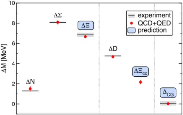
The low-energy spectrum and phenomenology of strongly-interacting particles is well described by Quantum Chromodynamics (QCD). Ab initio results have been obtained using Monte Carlo simulations of QCD regularized on the lattice, with a very good agreement with experiments. In particular, the mass pattern of an octet of light pseudoscalar mesons is well understood identifying them as pseudo Nambu–Goldstone bosons of spontaneous chiral symmetry breaking. A ninth pseudoscalar meson—the 𝜂′_{—evades this classification. It is associated to} flavour-singlet axial U(1) transformations, but it is too heavy to be a pseudo Nambu–Goldstone boson. This is known as the U(1)𝐴problem.

A solution to this problem was proposed by Witten and Veneziano in 1979. Their proposal links the 𝜂′_{mass to the anomaly in the flavour-singlet axial Ward–Takahashi identities. They} predict an anomalous contribution to the mass proportional to the topological susceptibility computed in Yang–Mills (YM) theory.

The verification of the Witten–Veneziano formula requires the computation of the YM topological susceptibility and the 𝜂′_{meson mass from first principles. This is possible only} solving QCD at the non-perturbative level, as for instance in lattice simulations. This thesis is a step toward the implementation and verification of the Witten–Veneziano formula on the lattice.

In the first part of the thesis, we computed the topological susceptibility with percent-level accuracy in the SU(3) YM theory and for the first time in the 𝑁c→ ∞ limit. The computation was done on the lattice implementing a naïve discretization of the topological charge evolved with the YM gradient flow. We provided a field-theoretical proof that the cumulants of the topological charge distribution computed using this definition coincide, in the continuum limit, with those of the universal definition appearing in the anomalous Ward–Takahashi identities. We performed a range of high statistics Monte Carlo simulations with different lattice spacings and 𝑁cvalues. The coverage of parameter space allowed us to extrapolate the topological susceptibility to the continuum and 𝑁c→ ∞ limits with confidence, keeping all systematic effects under control. As a by-product, we measured the non-Gaussianity of the topological charge distribution in SU(3) YM theory. This result is compatible with the expectations from the large-𝑁cexpansion, while it rules out the 𝜃 behaviour of the vacuum energy predicted by the dilute instanton gas model.

In the last part of the thesis, we focused on the direct lattice determination of the mass of the 𝜂′ _{meson. With state-of-the-art techniques, it is still not possible to compute this mass} with an adequate accuracy. The root of the issue is the exponential worsening with distance of the signal-to-noise ratio of correlation functions. This is a very general unsolved problem, which is currently limiting the accuracy of a broad class of Monte Carlo computations. We proposed to address this problem generalising the multilevel Monte Carlo algorithm to theories with dynamical fermions. We devised the first step of this program, namely the factorization of hadronic two-point functions, focusing on the disconnected contribution which is relevant to the 𝜂′_meson.

Acknowledgements

I would like to express my deep gratitude to my advisor Prof. Leonardo Giusti for his mentoring during the last four years. I thank him for introducing me to the topic of lattice QCD, for supporting me throughout the learning process and for his essential assistance in writing this thesis. I am indebted to him for the education that I received on how to approach physics problems, pursue research objectives and present the results.

Most of the original work that went into this thesis has been carried out in collaboration with Leonardo and other people, notably Stefan Schaefer and Miguel García Vera. It is a pleasure to share the credit for the results presented in this thesis with them.

I wish to thank the thesis referees Prof. Luigi Del Debbio and Prof. Uwe-Jens Wiese for sharing with me very helpful comments and corrections to the thesis, that I hope to have addressed in the final version.

I have been lucky to receive an education in high energy physics at Scuola Normale Superiore, following classes by Prof. Enrico Trincherini, Prof. Riccardo Barbieri, Dario Francia and many others. I am especially thankful to Enrico for allowing me to pursue a PhD program with Leonardo and other people not in Pisa.

Thanks to Alberto, Fabrizio, Luca and Stefano, together with many other people in Pisa and Milano, for any interesting discussion that contributed to form me as a physicist and a researcher.

Contents

The original contribution of the thesis 8

1. Quantum Chromodynamics 11

1.1. Gauge theories 11

1.1.1. The gauge theory with fermions 13 1.1.2. The path integral 14

1.2. Renormalization 15

1.2.1. Renormalization à la Wilson 16 1.2.2. The renormalization group 17 1.2.3. The 𝛬-parameter 18

1.2.4. Asymptotic freedom 19 1.2.5. RGI masses 20

1.2.6. Renormalization of composite fields 21 1.2.7. The operator product expansion 22 1.3. A couple of non-perturbative results 23 1.3.1. The spectrum of QCD 23

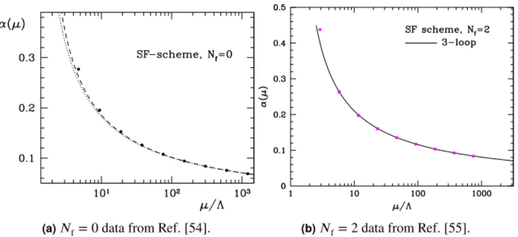
1.3.2. The running coupling in YM theory and 𝑁f= 2 QCD. 24 1.4. Chiral symmetry 26

1.4.1. Ward–Takahashi identities 28

1.4.2. Spontaneous symmetry breaking and Goldstone’s theorem 30 1.4.3. The GMOR relation 32

1.4.4. Chiral symmetry breaking in 𝑁f= 2 QCD 33

2. Lattice regularization 35

2.1. Gauge theories on the lattice 35 2.1.1. The lattice gauge field 37 2.1.2. Wilson’s plaquette action 39

2.2. Lattice fermions and chiral symmetry 39 2.2.1. The fermion doubling problem 40

2.2.2. Wilson fermions 42

2.2.3. Nielsen–Ninomiya no-go theorem 43

2.2.4. The Ginsparg–Wilson relation and Lüscher’s symmetry 44 2.2.5. Dirac operator spectrum 45

2.2.6. The overlap Dirac operator 46 2.3. The path integral on the lattice 47 2.3.1. The transfer matrix 48

2.3.2. Spectroscopy 50

2.3.3. Quark bilinears on the lattice 50 2.3.4. Lattice currents and densities 51 2.3.5. Approximate methods 52 2.4. Monte Carlo simulations 53 2.4.1. Importance sampling 54

2.4.2. The Monte Carlo for Yang–Mills theory 55 2.4.3. The Monte Carlo with fermions 55 2.4.4. Fermion correlators 57

2.5. The continuum limit 59 2.6. Symanzik’s effective theory 60 2.6.1. Lattice improvement 63

3. The flavour-singlet sector 65

3.1. The 𝜃-term 65

3.1.1. The topological charge 66

3.1.2. The distribution of the topological charge on the lattice 68 3.2. The anomalous U(1)𝐴 70

3.2.1. The anomalous U(1)𝐴with Ginsparg–Wilson fermions 70 3.2.2. Index theorem 72

3.2.3. The 𝜃-angle and the fermion mass matrix 73 3.2.4. Universal definition 73

3.3. The Witten–Veneziano mechanism 75 3.3.1. The 𝜂′_{mass formula 77}

3.3.2. Higher cumulants 77

3.4. Large-𝑁cin chiral perturbation theory 78

4. Topological charge with gradient flow 81

4.1. The Yang–Mills gradient flow in the continuum 81 4.2. Cumulants of the topological charge on the lattice 84 4.2.1. Ginsparg–Wilson definition of the charge density 84 4.2.2. Ginsparg–Wilson definition of cumulants 85 4.2.3. Universality at positive flow time 86

5. Lattice_SU(3)computation 89

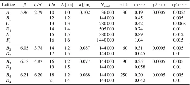
5.1. Numerical setup 89 5.1.1. Ensembles generated 89

Contents 5.1.3. Autocorrelation times 92 5.2. Physics results 93 5.2.1. Scale setting 93 5.2.2. Topological susceptibility 95 5.2.3. The ratio 𝑅 99 5.3. Conclusions 99

6. LatticeSU(𝑁_c)computation 101

6.1. Definition of the reference scale 𝑡0 102 6.2. Lattice details 102

6.2.1. Gradient flow observables 103 6.2.2. Topological susceptibility 104 6.2.3. Finite volume 105

6.2.4. Autocorrelations 105 6.3. Results 105

6.4. Conclusions 107

7. Noise reduction with multilevel integration 109

7.1. Signal-to-noise ratio of Monte Carlo observables 110 7.1.1. Variance of fermionic correlators 111

7.2. Domain decomposition and multilevel integration 113 7.2.1. Factorization of the path integral 114

7.2.2. The multilevel Monte Carlo algorithm 114

7.3. An application of multilevel integration to Yang–Mills theory 115 7.3.1. Domain decomposition of the Yang–Mills partition function 116 7.3.2. Factorization of the Wilson loop 117

7.3.3. Multilevel integration 118

8. Domain decomposition with fermions 121

8.1. Quark propagator and locality 122

8.2. Multilevel integration of the disconnected pseudoscalar propagator 123 8.2.1. Two-level integration 125

8.3. Numerical tests for the disconnected pseudoscalar propagator 126 8.3.1. Numerical results 127

8.4. Conclusions 130

9. Conclusions and outlooks 131

9.1. Additional results 132 9.2. Future developments 133

A. Conventions 135

A.1. The special unitary group SU(𝑁) 135 A.1.1. The Lie algebra 𝔰𝔲(𝑁) 135

A.1.2. The fundamental representation 136 A.1.3. The adjoint representation 137

A.2. The link differential operator 137 A.3. Dirac 𝛾-matrices 137

A.3.1. Chiral representation 138 A.3.2. Charge conjugation 138 A.4. Grassmann numbers 138 A.4.1. Wick’s theorem 140 A.5. The Haar measure 140 A.6. Wick’s rotation 141

B. Chiral perturbation theory 143

B.1. QCD with sources 144 B.2. The chiral Lagrangian 144 B.2.1. Beyond leading order 146

C. The transfer matrix 149

C.1. Quantum field theory Hilbert space 151 C.2. Transfer matrix operator 152

D. The1/𝑁_cexpansion 153

D.1. Hadrons in the 1/𝑁cexpansion 155

D.2. The 𝜃-angle dependence in the 1/𝑁cexpansion 157

E. Instantons 159

E.1. The BPST instanton 161 E.2. Other gauge groups 163

E.3. The dilute instanton gas model 163

F. Runge–Kutta–Munthe-Kaas integrators 167

F.1. Application to the Yang–Mills gradient flow 168

List of publications

For an updated list see

https://inspirehep.net/author/profile/M.Ce.1

Articles

[1] M. Cè, C. Consonni, G. P. Engel and L. Giusti, ‘Non-Gaussianities in the topological charge distribution of the SU(3) Yang-Mills theory’, Phys. Rev. D 92, 074502 (2015), arXiv:

1506.06052 [hep-lat]

[2] M. Cè, L. Giusti and S. Schaefer, ‘Domain decomposition, multilevel integration, and exponential noise reduction in lattice QCD’, Phys. Rev. D 93, 094507 (2016), arXiv:

1601.04587 [hep-lat]

[3] M. Cè, M. García Vera, L. Giusti and S. Schaefer, ‘The topological susceptibility in the large-𝑁 limit of SU(𝑁) Yang-Mills theory’, Phys. Lett. B 762, 232–236 (2016), arXiv:

1607.05939 [hep-lat]

[4] M. Cè, L. Giusti and S. Schaefer, ‘A local factorization of the fermion determinant in lattice QCD’, (2016), arXiv:

1609.02419 [hep-lat]

Proceedings

[5] M. Cè, C. Consonni, G. P. Engel and L. Giusti, ‘Testing the Witten-Veneziano mechanism with the Yang-Mills gradient flow on the lattice’, PoS LATTICE2014, 353 (2014), arXiv:

1410.8358 [hep-lat]

[6] M. Cè, ‘Non-Gaussianity of the topological charge distribution in SU(3) Yang-Mills theory’, PoS LATTICE 2015, 318 (2015), arXiv:

1510.08826 [hep-lat]

topo-logical susceptibility of Yang-Mills gauge theory’, PoS LATTICE2016, 350 (2016), arXiv:

1610.08797 [hep-lat]

[8] M. Cè, L. Giusti and S. Schaefer, ‘Domain decomposition and multilevel integration for fermions’, PoS LATTICE2016, 263 (2016), arXiv:

1612.06424 [hep-lat]

Introduction

The quantum theory of fields (QFT) is the theoretical framework that, since the second half of the twentieth century, has been successfully used to construct modern theories of high energy physics. It is the only known way to combine quantum dynamics with the theory of special relativity. The Standard Model (SM) of particle physics [9–11] is a self-consistent QFT which represents the current reference in the understanding of subatomic particles and their interactions. It describes three of the four known fundamental forces of nature—strong, weak and electromagnetic interactions—by means of a quantum gauge theory. That is to say, a QFT in which the Lagrangian is invariant under a continuous group of local transformations, forming the Lie group SU(3) × SU(2) × U(1). The non-Abelian SU(3) subgroup describes strong interactions mediated by gauge bosons called gluons and the corresponding gauge theory is called Quantum Chromodynamics (QCD) [12, 13]. Of the SM elementary fermions, only those called quarks carry the colour non-Abelian charge and thus ‘feel’ the strong interactions, in contrast with the leptons, which are colour-neutral.

In the functional integral formulation of QFT, the path integral of QCD is, in a formal and very compact notation,

𝒵 = ∫𝒟[ ̄𝜓,𝜓,𝐴]exp{i𝑆[ ̄𝜓,𝜓,𝐴]}, (0.1) where 𝜓 ( ̄𝜓) denotes the quark field (and its Dirac adjoint) and 𝐴 the gluon field. 𝒟[ ̄𝜓, 𝜓, 𝐴] denotes the functional integration measure and 𝑆[ ̄𝜓, 𝜓, 𝐴] is the action of QCD, a functional of the fields that can be split into the fermion action

𝑆f[ ̄𝜓, 𝜓, 𝐴] = ∫d4𝑥 ̄𝜓(𝑥)[i /𝐷[𝐴] − 𝑀]𝜓(𝑥) (0.2) and the gluon action

𝑆g[𝐴] = − 1_{4𝑔2∫ d}4𝑥 𝐹𝜇𝜈𝑎(𝑥)𝐹𝑎𝜇𝜈(𝑥). (0.3) QCD is the subject studied in the thesis, and from now on we focus on it.

Asymptotic freedom

Even though QCD is superficially similar to Quantum Electrodynamics (QED), the Abelian gauge theory of electromagnetic interactions, the phenomenology of the two theories differs substantially. This is mainly due to the fact that non-Abelian gauge theories like QCD, in which the force-carrying gauge bosons are themselves charged under the gauge group, are

asymptotically free theories [14, 15]. The strength of interactions, determined by the coupling 𝑔,

becomes asymptotically weaker as energy increases, in contrast with QED in which the vacuum 1

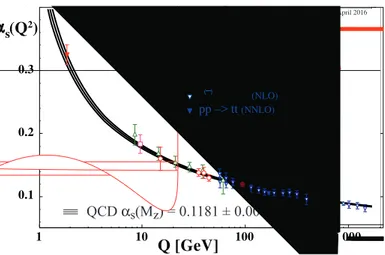
Figure 0.1.:_{Summary of experimental measurements of 𝛼𝑠= 𝑔}2_{/4π as a function of the energy scale 𝑄.}

The respective order of QCD perturbation theory used in the extraction of 𝛼𝑠is indicated in

brackets. The fit is performed including experimental determinations based on (at least) full NNLO QCD prediction and non-perturbative lattice determinations. The fit line shows the running of 𝛼𝑠using the MS-scheme four-loop 𝛽-function and three-loop threshold matching at

charm-, bottom- and top-quark pole masses.

polarization screens the electric charge at long distance. In mathematical terms, the change of the coupling 𝑔 with energy is encoded in the so-called 𝛽-function

𝛽(𝑔) = 𝑄 𝜕𝑔_{𝜕𝑄 = −(𝑏}0𝑔3+ 𝑏1𝑔5+ ⋯ ), 𝑏0= 1_16π2(11_{3 𝑁}c− 23𝑁f), (0.4) for a theory with SU(𝑁c) gauge group and 𝑁fflavours of quarks in the fundamental repres-entation. Asymptotic freedom is realized with a negative 𝛽-function for 𝑔 → 0, e.g. in QCD (𝑁c= 3 case) if the number of flavours is 𝑁f ≤ 16, which obviously include the physical case.

It is worth noting that even the theory without fermions (𝑁f = 0), described only by the gluon action in Eq. (0.3), is an asymptotically free theory. This purely-bosonic quantum gauge theory is know as Yang–Mills (YM) theory, as it was firstly proposed by Yang and Mills [16] for the SU(2) gauge group. Unlike the Abelian counterpart, which describes a free photon, YM theory is naturally interacting, with interactions completely determined just by the non-Abelian structure of gauge symmetry.

Perturbative methods based on Feynman diagrams treat interactions as a small perturbation of otherwise free particles. Asymptotic freedom allows perturbation theory to be used to describe the dynamics of quarks and gluons at extremely high energies. The perturbative expansion parameter 𝛼𝑠= 𝑔2/4π is small in this regime and, to a given order in perturbation theory, the running given by the 𝛽-function in Eq. (0.4) can be integrated. For instance, at leading order

𝛼𝑠(𝑄) = 𝑔 2_(𝑄) 4π ≃ _𝑏0ln1𝑄2 𝛬2 QCD , (0.5)

from which is clear that the strength of interactions changes logarithmically with the energy. Here, 𝛬QCD≈ 300 MeV is an integration constant whose precise value depends on the renor-malization scheme. It sets a scale at which the perturbative 𝛼𝑠formally diverges: this means that perturbation theory is not reliable at energies 𝑄 ≈ 𝛬QCD, and non-perturbative methods are needed.

Figure 0.1 shows how very different experimental measurements at different scales 𝑄, matched with different order of perturbation theory, give values of 𝛼𝑠(𝑄) that reproduce the correct perturbative running. These measurements concur together with lattice results to give the average value of 𝛼𝑠, in the MS scheme, at the energy scale 𝑀𝑍≈ 91 GeV [17]

𝛼MS

𝑠 (𝑀𝑍2) = 0.1181(11). (0.6) An introduction to QCD, including renormalization, is given in Chapter 1.

Hadrons

Asymptotic freedom indicates that at lower energies the interactions become so strong that a perturbative approach is not applicable, since the dynamics is not approximated at all by free quarks and gluons. Indeed, the existence of quarks and gluons has been indirectly confirmed identifying them as the constituents, the partons, of composite particles called hadrons—such as the proton and the neutron—when scattered at high energies. However, neither free quarks nor free gluons have been observed directly in high energy physics experiment. This phenomenon is called colour confinement and asserts that all the asymptotic states present in the spectrum must be colour singlet.

A simple state which transforms trivially under SU(3) colour transformations can be obtained in two ways. A meson is a bound state obtained combining a quark and an antiquark which transform respectively under the fundamental 𝟑 and antifundamental ̄𝟑 representation

colour: 𝟑 ⊗ ̄𝟑 ⊃ 𝟏 of mesons. (0.7) A baryon (antibaryon) is a bound state obtained combining three (anti)quarks in the (anti)fun-damental representation

colour: 𝟑 ⊗ 𝟑 ⊗ 𝟑 ⊃ 𝟏 of baryons. (0.8) More complicated colour-singlet states, such as tetraquarks and pentaquarks, may exist as bound states. Even in the absence of quarks, in the YM theory case, it is still possible to obtain a

glueball colour-singlet state made only of gluons. Glueballs form the spectrum of all excited

states in YM theory. Despite being colour-neutral, hadrons and glueballs feel residual strong interactions in the form of nuclear interactions. These are in analogy with the van der Waals forces between electrically-neutral molecules.

Remarkably, the dynamics behind confinement generates a mass gap in the theory. Even if the elementary fields in the Lagrangian are massless, there are no massless particles in the spectrum, with the only exception of the NG bosons of chiral symmetry breaking if two or more flavours of massless quarks are present. The analytical proof of the fact that YM theory has a mass gap is an unsolved Millennium Prize problem [18]. In QCD, the strong dynamics 3

accounts for most of the mass of hadrons made of light quarks, which is typically ≈ 1 GeV. With the only exception of an octet of pseudoscalar mesons which are significantly lighter, these masses are proportional to the characteristic energy scale 𝛬QCDwith an 𝒪(1) coefficient. It is clear from Figure 0.1 that a perturbative expansion in 𝛼𝑠fails at these energy scales, thus a complete understanding of the hadron spectrum and colour confinement must come from a non-perturbative approach to the theory.

Lattice

Until 1974, no methods were available to make quantitative predictions for the low-energy regime. The introduction by Wilson [19] of a regularization of QCD on a spacetime lattice first opened the way to fully non-perturbative predictions. The use of Euclidean spacetime allows the direct application to QFT of Monte Carlo methods used in statistical mechanics and the study of non-perturbative phenomena through numerical simulations. Moreover, on the theoretical side, the lattice-regularized path integral is mathematically well-defined. In particular, gauge theories can be discretized in a way that gauge invariance is exactly preserved and gauge fields are angular variable, which makes gauge fixing unnecessary. In the thesis, we use the lattice regularization to study non-perturbative phenomena in QCD and YM theory. This formalism is introduced in Chapter 2.

Flavour

Besides colour, quarks are labelled by another quantum number called flavour which denotes the presence of more than one species of them. From the point of view of QCD, flavour is a global quantum number and it is not associated to a force mediated by a gauge boson. Six different flavours exist and, neglecting for the moment the difference between quark masses, the theory is completely blind to flavour, which thus generates a global SU(6) symmetry. However, the electroweak sector of the Standard Model breaks flavour symmetry in two ways. First, the six quarks are embedded in pairs in three generations of weak doublets. The doublet components have different electric charge and weak interactions allow transitions between different flavours. Still, these effects provide only a small correction to the dynamics of coloured states: electromagnetic interactions have a coupling 𝛼 ≈ 1/137 which is much smaller with respect to the strong coupling in Eq. (0.6); weak interactions at ≈ 1 GeV are well described by irrelevant four-fermion operators proportional to the Fermi coupling 𝐺F, suppressed by the electroweak symmetry breaking scale 𝑣

𝐺F≡ 1

√2𝑣2, 𝑣 ≈ 246 GeV. (0.9) A second more important fact is that electroweak spontaneous symmetry breaking is re-sponsible for the mass of elementary fermions, including quarks, and the range of masses is widespread1

1_{The values quoted here are [17]: running masses ̄𝑚}MS

𝐼3 𝑄 𝑆 𝜂′ 𝑞 ̄𝑞 𝜋0_{, 𝜂} 𝑢 ̄𝑑𝜋 + 𝑢 ̄𝑠𝐾 + 𝑑 ̄𝑠 𝐾0 𝑑 ̄𝑢 𝜋− 𝑠 ̄𝑢 𝐾− 𝑠 ̄𝑑 _̄ 𝐾0

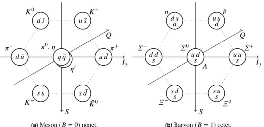
(a)Meson (𝐵 = 0) nonet.

𝐼3 𝑄 𝑆 𝑢 𝑑_𝑠 𝛴0 𝛬 𝑢 𝑢_𝑠 𝛴+ 𝑢 𝑢_𝑑 𝑝 𝑑 𝑢_𝑑 𝑛 𝑑 𝑑_𝑠 𝛴− 𝑠 𝑑 𝑠 𝛯− 𝑠 𝑢𝑠 𝛯0 (b)Baryon (𝐵 = 1) octet.

Figure 0.2.:Eightfold Way particle multiplets. Particles along the same horizontal line share the same strangeness 𝑆, while those on the same vertical line share the same isospin projection 𝐼3.

Electric charge, given by the Gell-Mann–Nishijima formula 𝑄 = 𝐼3+1/2(𝐵 +𝑆), is represented

on a diagonal axis.

𝑚𝑢≈ 2.15(15) MeV, 𝑚𝑐≈ 1.67(7) GeV, 𝑚𝑡≈ 174.2(14) GeV,

𝑚𝑑≈ 4.70(20) MeV, 𝑚𝑠≈ 93.8(24) MeV, 𝑚𝑏≈ 4.78(6) GeV. (0.10)

1 MeV 1 GeV 1 TeV

𝑚𝑢 𝑚𝑑 𝑚𝑠 𝛬QCD 𝑚𝑐 𝑚𝑏 𝑚𝑡

These numbers have to be taken with some care. Indeed, they are not true particle masses since quarks, because of confinement, do not exists as asymptotic states of the interacting QFT. They are parameters of the Lagrangian of the theory, which are not observable and can be precisely defined only after fixing some renormalization scheme. The mass of three of the six flavours of quarks—charm, bottom and top—is higher than the scale of strong interactions, thus when considering light hadrons it is a good approximation to integrate out and completely neglect them.

On the other hand, the mass of the up and down quarks is much smaller than the strong scale 𝛬QCD, and so is their mass splitting. Therefore, SU(2) flavour rotations acting on the up and down quarks leaves the action almost invariant. This manifests itself as an approximate symmetry of the spectrum: mesons and baryons containing up and down quarks are organized in multiplets of representations of SU(2)𝐼classified by the so-called isospin quantum number, by analogy with three-dimensional rotations classified by spin.

The mass of the strange quark is approximatively smaller but comparable with the strong scale. Nevertheless, it is worth studying the transformation properties of hadrons under the SU(3)𝐹 flavour group. This was noticed even before the introduction of QCD and gave rise to a group-theoretical classification of hadrons know as Eightfold Way [20, 21]. For instance, combining an up, down or strange quark with an antiquark we can obtain nine different pseudoscalar mesons. The lightest eight—three pions, four kaons and the 𝜂—are nicely organized in an octet 5

Table 0.1.:The nonet of mesons with pseudoscalar quantum numbers: 𝐽𝑃 = 0−. The columns show

respectively the transformation properties under SU(3)𝐹and SU(2)𝐼, the valence quark content

and the mass from Ref. [17]. The 𝜂 and 𝜂′_{mesons are orthogonal linear combinations of the}

octet meson 𝜂𝟖and the singlet meson 𝜂𝟏given by

𝜂𝟖= (𝑑 ̄𝑑+ 𝑢 ̄𝑢 − 2𝑠 ̄𝑠)/√6,

𝜂𝟏= (𝑑 ̄𝑑+ 𝑢 ̄𝑢 + 𝑠 ̄𝑠)/√3,

𝜃 ≈ −11.4°.

Meson Quark content Mass [MeV]

𝟖 𝟑 𝜋 + _{𝑢 ̄𝑑 139.570 18(35)} 𝜋0 _{(𝑑 ̄𝑑− 𝑢 ̄𝑢)/√2 134.9766(6)} 𝜋− _{𝑑 ̄𝑢 139.570 18(35)} 𝟐 𝐾_𝐾+0 𝑢 ̄𝑠_{𝑑 ̄𝑠} 493.677(16)_497.611(13) 𝟐 _𝐾𝐾̄−0 𝑠 ̄𝑑_{𝑠 ̄𝑢} 497.611(13)_493.677(16) mixing 𝟏 𝜂 𝜂𝟖cos 𝜃 + 𝜂𝟏sin 𝜃 547.862(17) 𝟏 𝟏 𝜂′ _−𝜂 𝟖sin 𝜃 + 𝜂𝟏cos 𝜃 957.78(6) representations of flavour, while the ninth—the 𝜂′_{—transforms as a singlet}

flavour: 𝟑 ⊗ ̄𝟑 = 𝟖 ⊕ 𝟏 of pseudoscalar mesons. (0.11) The organization of this nonet of pseudoscalar mesons under representations of SU(3)𝐹 is pictured in Figure 0.2a, where it is also suggested how the nonet decomposes under the SU(2)𝐼 isospin subgroup. The same information is given in Table 0.1 along with the experimental values of the pseudoscalar meson masses.

In the baryon case, the combination of three up, down or strange (anti)quarks decomposes in flavour: 𝟑 ⊗ 𝟑 ⊗ 𝟑 = 𝟏𝟎 ⊕ 𝟖 ⊕ 𝟖 ⊕ 𝟏 of baryons (antibaryons). (0.12) Fermi–Dirac statistics allows only for a spin-3/₂decuplet and a spin-1/₂octet. The latter, which

includes the nucleons, is pictured in Figure 0.2b.

Chiral symmetry

In the limit in which the mass of 𝑁fflavours of quarks is sent to zero, the theory is symmetric under a larger group of transformations, acting on left- and right-handed chiral components of Dirac fermions independently. This is called chiral symmetry and is described by the group SU(𝑁f)𝐿× SU(𝑁f)𝑅. SU(𝑁f)𝐹flavour symmetry manifests itself as the vectorial subgroup of the chiral symmetry group.

Chiral symmetry of the massless theory is spontaneously broken by the strong dynamics: the order parameter is a non-zero chiral condensate

⟨ ̄𝑞𝑞⟩ ∼ 𝛬3

QCD. (0.13)

The dynamically generated chiral condensate is left invariant by the vectorial flavour subgroup, which thus still classifies the spectrum of the theory. Moreover, the Goldstone theorem predicts the presence in the theory spectrum of 𝑁2

f − 1 massless NG bosons, which are identified with a multiplet of pseudoscalar mesons fitting an adjoint representation of SU(𝑁f).

In the real world no quark flavours are exactly massless and thus chiral symmetry is broken also explicitly. Nevertheless, if the breaking induced by quark masses is small, approximate chiral symmetry is still relevant to the dynamics of the lightest states. In the 𝑁f = 2 case, it explains why the isospin triplet of pions is almost an order of magnitude lighter than other mesons and hadrons: they would be massless NG bosons in the limit 𝑚𝑢, 𝑚𝑑 → 0, and the smallness of these quark masses compared to 𝛬QCDconstrains the pion masses to be small. In the 𝑁f = 3 case, the strange quark mass breaks chiral symmetry in a substantial way, but it is still possible to relate to the chiral dynamics the comparatively small masses, reported in Table 0.1, of the octet of pseudoscalar mesons pictured in Figure 0.2a.

Singlet

In addition to SU(𝑁f)𝐿× SU(𝑁f)𝑅chiral symmetry, the massless limit of QCD at the classical level has another global symmetry, described by the phase rotations U(1)𝐿× U(1)𝑅acting on the left- and right-handed chiral components in a flavour-independent way. The vector rotation of this flavour-singlet transformation is an exact symmetry of the theory, responsible for the conservation of the baryon number. On the contrary, the U(1)𝐴axial rotation has a peculiar phenomenology. Indeed, it is evident from Table 0.1 that the mass of the 𝜂′_{pseudoscalar meson,} which is identified as an almost flavour singlet combination, is ≈ 1 GeV and comparable to the mass of baryons. The effective theory of chiral symmetry breaking is not sufficient to explain the mass of the 𝜂′_{. The missing ingredient is that the U(1)}

𝐴symmetry is anomalous: even in the chiral limit it is explicitly broken by quantum effects, not present in the classical theory.

Studying the theory regularized on the lattice is not the only way to explore QCD at the non-perturbative level. Large-𝑁ctechniques [22] exploit the simplification of QCD when the number of colours 𝑁cis sent to infinity. Notably, in this limit the anomaly responsible for the breaking of U(1)𝐴symmetry vanishes. Witten [23] and Veneziano [24, 25] used this fact to obtain a formula to compute the anomalous contribution to the flavour-singlet meson mass, up to corrections of 𝒪(1/𝑁c) 𝐹2 𝜋 2𝑁f𝑀 2 𝜂′= 𝜒𝑡YM. (0.14) The quantity in the r.h.s. of this formula is the topological susceptibility of YM theory, i.e. com-puted in the theory with 𝑁f= 0. In Chapter 3 we review the properties of U(1)𝐴transformations, both in the continuum and on the lattice, and we give a derivation of the Witten–Veneziano formula in Eq. (0.14).

The original contribution of the thesis

The work of the thesis inserts in a long-time project of verifying the Witten–Veneziano formula using the lattice discretization of QCD. Since the mass of a meson is experimentally accessible, it is possible to check the approximate validity of Eq. (0.14) computing on the lattice the YM topological susceptibility and comparing it with the experimental value of 𝑀𝜂′. However,

Eq. (0.14) is an exact field-theoretic relation only in the chiral limit and in the limit 𝑁c→ ∞. Clearly, the experimental mass of the 𝜂′_{meson is not given in this limit.}

We aim to compute both sides of Eq. (0.14) from first principles. The validity of the Witten– Veneziano formula relies on quantization, since the anomaly is a pure quantum effect, and falls in the non-perturbative regime of the theory. Therefore, without even assuming QCD, the quantitative verification of Eq. (0.14) would provide a check of quantization of the theory at the non-perturbative level. Clearly, this program is possible only using lattice regularization and simulations. As a bonus, the lattice framework allows the total control of the theory parameters, including the number of colours, the number of quark flavours and quark masses.

The original material of the thesis is dived in two parts: the first part has to do with the topological susceptibility in the r.h.s. of Eq. (0.14), and solves the problem with a computation of 𝜒YM

𝑡 in the large-𝑁climit to the percent level. The second part concerns the direct lattice computation of 𝑀𝜂′. With the present techniques, the computational challenge to obtain

𝑀𝜂′with an acceptable statistical accuracy is not affordable. The thesis addresses this issue

conceptually, proposing a new strategy to compute the 𝜂′_mass.

Part I: the topological susceptibility in Yang–Mills theory

The topological susceptibility is the variance of the distribution of the topological charge, which is quantity of non-perturbative nature. Therefore, this observable is an excellent candidate to be computed with lattice methods. Nevertheless, as explained in Chapter 3, the definition of the topological charge on the lattice is not free of obstruction. The clash between chiral symmetry and lattice regularization [26] implies a complex renormalization of the topological charge and the topological susceptibility that invalidates the Ward identities behind the Witten–Veneziano mechanism. Only in recent years a method to correctly define the topological charge and its cumulants on the lattice has been found [27], based on a Dirac fermion operator satisfying the Ginsparg–Wilson (GW) relation [28]. This lattice discretization of the topological charge and its properties are addressed in Chapter 3. The downside is that this method is very expensive in terms of computational resources.

In Chapter 4 we introduce a different lattice discretization of the topological charge, based on the YM gradient flow [29]. We prove that the cumulants of the topological charge distribution defined at positive flow time have a proper continuum limit which satisfies the anomalous chiral WTIs [1]. Employing this discretization, in Chapter 5 we present the results of a high-statistics computation of the second – i.e. the susceptibility – and fourth cumulants of the topological charge distribution in SU(3) YM theory [1]. In Chapter 6 we extend the computation of the susceptibility at SU(𝑁c) YM theory, up to 𝑁c= 6, in order to extract with confidence the value of the topological susceptibility in the 𝑁c→ ∞ limit [3]. This is the proper value to insert in the r.h.s. of Eq. (0.14).

The original contribution of the thesis

Part II: the flavour-singlet pseudoscalar meson mass

The lattice computation of 𝑀𝜂′is an open problem. Indeed, it is practically not possible to obtain

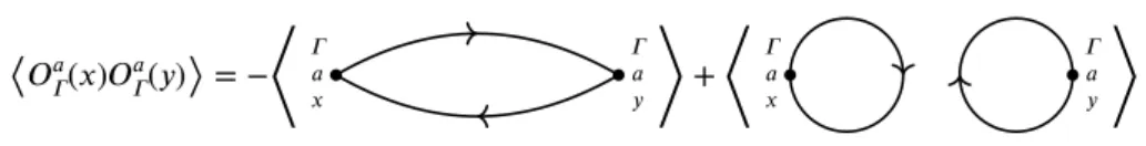
the mass of the flavour-singlet pseudoscalar with a traditional approach, from the exponential decay rate at asymptotic distances of the proper two-point function. The reason is a very general problem with the signal-to-noise ratio of correlation functions: the statistical error decays asymptotically with a lower rate with respect to the signal. Therefore, with a standard Monte Carlo algorithm, the computational cost to extract the signal at longer distances maintaining the same statistical accuracy increases exponentially. This problem is particularly bad in the case of the flavour-singlet propagator, since it contains disconnected quark diagrams whose error do not decrease at all with distance. In Chapter 7 we state precisely this problem and introduce a method which has been successfully applied to bosonic theories: the multilevel Monte Carlo algorithm [30–32].

Multilevel integration requires the decomposition in space-time domains of the action and the observables, but an exact factorization is not possible if the theory contains fermions. We par-tially solve this problem introducing an approximate factorization for fermionic observables [2]. The exact result is easily recovered with a simple modification of the multilevel Monte Carlo algorithm. The application of this method to the disconnected contribution of the flavour-singlet propagator is particularly simple. We present the factorization of the disconnected contribution in Chapter 8, including numerical evidence obtained in the quenched theory that shows an exponential gain in the signal-to-noise ratio.

The factorization of the action has been obtained meanwhile in Ref. [4]. Therefore, the combination of the factorization of the propagator presented in Chapter 8 and the action in Ref. [4] paves the way to multilevel simulations with fermions. These in turn are a candidate solution to a broad class of signal-to-noise problems, including the flavour-singlet propagator.

1. Quantum Chromodynamics

QCD is a renormalizable gauge theory with SU(3) gauge group. Gauge theories are a special class of QFT in which the Lagrangian is manifestly invariant under a local group of fields transformations.

In this chapter, we introduce gauge theories working in Euclidean spacetime, in contrast with usual Minkowski spacetime. For this reason, the expressions introduced in this section differ from the ones in the Introduction. A QFT in Minkowski spacetime is mapped to a Euclidean one by a procedure called Wick’s rotation, which involves the substitution 𝑥4≡ i𝑥0and others summarized in Section A.6. Whether or not it is possible to analytically continue a QFT from real to imaginary time is not obvious. The criteria to be satisfied were given by Osterwalder and Schrader [33, 34]. In particular, a QFT in Euclidean spacetime must satisfy the so-called

reflection positivity to correspond to a well-defined QFT in Minkowiski spacetime. The use of

Euclidean spacetime is preparatory to Chapter 2, where the lattice discretization is applied, for technical reasons, to the Euclidean theory.1

After imposing gauge symmetry, the structure of the QFT is very constrained. In fact, once a gauge group is chosen and the field content is given, the request of renormalizability completely defines the action of QCD. In Section 1.1 we introduce the action of a non-Abelian SU(𝑁c) gauge theory with 𝑁fspecies of Dirac fermions and we quantize it in the path integral formalism. Then, in Section 1.2 we complete the building of this QFT renormalizing it. To conclude the chapter, Section 1.4 is dedicated to chiral symmetry.

1.1. Gauge theories

To introduce the action, we specify the criteria that define the gauge theory. In this thesis, we work with gauge theories with gauge group SU(𝑁c), where 𝑁c≥ 2 is the unspecified number of colours. This includes the physical case of QCD, which is easily obtained specifying 𝑁c= 3. However, as we will show, it is sometimes useful to consider gauge theories with a different number of colours.

The minimal gauge theory is Yang–Mills theory, which contains only one multicomponent field, 𝐴𝑎

𝜇(𝑥). This field possesses a Lorentz index 𝜇 and an internal colour index 𝑎. In spite of this, 𝐴𝑎

𝜇is not a proper Lorentz vector [35]. The Lorentz transformation properties are entangled with the internal gauge invariance. A proper Lorentz vector describes a spin-1 massive particle, with three internal degrees of freedom. The massless limit is singular: a massless particle has only two degrees of freedom with helicity ±1. Gauge invariance is necessary for the field 𝐴𝑎

𝜇(𝑥) to describe massless particles.

1_{In the following, we use improperly Poincaré symmetry to denote the ISO(4) group of isometries of Euclidean}

spacetime. Similarly, with Lorentz transformation rules we refer to transformation rules under the homogeneous subgroup SO(4).

From the gauge-group point of view, 𝐴𝑎

𝜇(𝑥) transforms under the adjoint 𝑁c2− 1-dimensional representation of the non-Abelian gauge group. This gives rise to a 𝑁2

c − 1 multiplicity of massless gauge bosons. In the defining representation, a generic gauge transformation is represented by a unitary 𝑁c× 𝑁cmatrix with unit determinant 𝛺(𝑥) for each spacetime point 𝑥, which can also be written as the exponential of a Hermitian traceless 𝑁c× 𝑁c matrix 𝜆(𝑥) ≡ 𝜆𝑎_(𝑥)𝑇𝑎

𝛺(𝑥) = exp{i𝜆𝑎_(𝑥)𝑇𝑎_{}. (1.1)} Here, 𝑇𝑎_{for 𝑎 = 1, … , 𝑁}2

c−1 are the Hermitian generators of SU(𝑁c) introduced in Section A.1, and the 𝜆𝑎_{(𝑥) parametrize the gauge transformation. In this representation, the gauge field is} represented by a Hermitian traceless matrix 𝐴𝜇≡ 𝐴𝑎𝜇𝑇𝑎, which transforms inhomogeneously under the gauge group

𝐴𝜇(𝑥) → 𝐴′𝜇(𝑥) = 𝛺(𝑥)[𝐴𝜇(𝑥) + i𝜕𝜇]𝛺†(𝑥). (1.2) The action is built as a functional of 𝐴𝜇and derivatives of 𝐴𝜇on the basis of symmetry considerations. It has to be invariant under local gauge transformations. A proper field derivative is given by the field strength tensor

1.1. Gauge theories

Other terms, such as a mass term tr{𝐴𝜇𝐴𝜇}, are not allowed by the requirement of gauge invariance. In contrast with the Abelian case, this is not a free theory: it is evident from Eq. (1.3) that 𝐹𝜇𝜈contains a term quadratic in 𝐴𝜇. Therefore, the action in Eq. (1.7) implicitly includes interactions between three and four gauge bosons. Remarkably, symmetry alone completely dictates the structure of these interactions. The only free parameters are two dimensionless

bare couplings, 𝑔0and 𝜃.

The second term in Eq. (1.7) is the so-called 𝜃-term. It has peculiar properties, which will be described in details in Chapter 3. For the moment, it suffices to notice that excluding this last term the Euclidean action is real. The 𝜃-term is purely imaginary instead: this is because it contains an odd number of times derivatives, differently from every other terms, that results in an extra i factor after Wick’s rotation. In the physical world, 𝜃 ≲ 1 × 10−10_{, as we will motivate} in Chapter 3. For this reason, in the following we restrict to the case 𝜃 = 0. This implies a real action which can be easily shown to be bounded from below.

1.1.1. The gauge theory with fermions

Physical gauge theories include additional matter fields besides 𝐴𝜇. These can be Dirac or Weyl fermions or scalars, in any representation of the gauge group. In this thesis, we focus to the case that includes QCD: the gauge theory of 𝑁fDirac fermions transforming under the fundamental representation of SU(𝑁c). The 𝑁fspecies are labelled by flavour.

This choice excludes the electroweak sector of the SM, which contains Weyl fermions and scalars. Also, we do not consider representations different from the fundamental for matter fields. These are common in models of physics beyond the SM.

A Dirac fermion transforms under a reducible3_{representation of the Lorentz group. It is} represented by a multicomponent Dirac spinor field 𝜓(𝑥). As a Dirac spinor, this field is a four-component vector in Dirac 𝛾-matrices space. The convention used for Dirac 𝛾-matrices is given in Section A.3. On top of this, 𝜓(𝑥) has internal indices: it is a 𝑁c-component vector transforming under the fundamental 𝑵crepresentation of SU(𝑁c). Moreover, when 𝑁f≥ 2, we use the notation 𝜓(𝑥) to denote a vector of 𝑁ffields: 𝜓 = (𝜓𝑢, 𝜓𝑑, 𝜓𝑠, … ).

To write the fermion action, it is useful to introduce the Dirac adjoint spinor field ̄𝜓(𝑥) ≡ 𝜓†_(𝑥)𝛾

4, (1.8)

which transforms under the antifundamental ̄𝑵c representation of SU(𝑁c). Scalar gauge-invariant field monomials are built contracting spinor, Lorentz and gauge indices in bilinear of 𝜓 and ̄𝜓. Ignoring the flavour structure, there are only two of them with 𝑑 ≤ 4

̄𝜓(𝑥)𝜓(𝑥), ̄𝜓(𝑥)𝛾𝜇𝜕𝜇𝜓(𝑥). (1.9) The action of free Dirac fermions with a global SU(𝑁c) symmetry is composed just of these two terms

𝑆free

f [ ̄𝜓, 𝜓] = ∫d4𝑥 ̄𝜓(𝑥)[/𝜕 + 𝑀0]𝜓(𝑥), /𝜕 ≡ 𝛾𝜇𝜕𝜇, (1.10) where 𝑀0is a 𝑁f× 𝑁fmatrix of bare fermion masses. Other terms, such as four-fermion fields, are excluded either by symmetries or by renormalizability. In view of the path integral approach

3_{The representation is reducible in even spacetime dimensions.}

to quantization, it is convenient to consider the action as a functional of independent 𝜓(𝑥) and ̄𝜓(𝑥) fields.

Interactions with gauge bosons are introduced requiring 𝜓 and ̄𝜓 to be invariant under local gauge transformations

𝜓(𝑥) → 𝜓′_{(𝑥) = 𝛺(𝑥)𝜓(𝑥), (1.11a)} ̄𝜓(𝑥) → ̄𝜓′_{(𝑥) = ̄𝜓(𝑥)𝛺}†_{(𝑥). (1.11b)} While the first term in Eq. (1.9) is still invariant under transformation rules in Eqs (1.11), the second term is not: the spacetime derivative acting on 𝛺(𝑥) generates an extra term. A gauge-covariant derivative field 𝐷𝜇𝜓(𝑥) is obtained applying the covariant derivative in Eq. (1.4) to 𝜓(𝑥)

𝐷𝜇𝜓(𝑥) = 𝜕𝜇𝜓(𝑥) − i𝐴𝜇(𝑥)𝜓(𝑥), 𝐷𝜇𝜓(𝑥) → [𝐷𝜇𝜓]′(𝑥) = 𝛺(𝑥)𝐷𝜇𝜓(𝑥), (1.12) where 𝜓(𝑥) and 𝐴(𝑥) are transformed according to Eqs (1.11a) and (1.2) respectively. Therefore, the gauge-invariant fermion action is

𝑆f[ ̄𝜓, 𝜓, 𝐴] = ∫d4𝑥 ̄𝜓(𝑥)[ /𝐷 + 𝑀0]𝜓(𝑥), (1.13) where

/𝐷 ≡ 𝛾𝜇𝐷𝜇 (1.14)

is the interacting Dirac operator.

The fermion action in Eq. (1.13) together with the bosonic action in Eq. (1.7) describes a theory of Dirac fermions with non-Abelian interactions

𝑆[ ̄𝜓, 𝜓, 𝐴] = 𝑆g[𝐴] + 𝑆f[ ̄𝜓, 𝜓, 𝐴]. (1.15) Like autointeractions between gauge bosons, also the interactions of fermions with one gauge boson are completely determined by symmetry principles alone. Restricting to the 𝜃 = 0 case, the only parameters are a dimensionless bare gauge coupling 𝑔0and the bare fermion mass matrix 𝑀0.

1.1.2. The path integral

We proceed to quantize the theory. The canonical quantization of gauge theories is highly non-trivial. The cleanest way to quantize a QFT with local gauge invariance is called BRST

quantization, and involves the rewriting of gauge invariance as global symmetry, depending

on an anticommuting parameter and acting on an extended field content. This includes colour-charged scalar fields with Fermi–Dirac statistics 𝑐 ( ̄𝑐) called (anti)ghosts.

In the thesis, we avoid these complications using the path integral or functional approach to quantization. We start introducing the formal expression for the path integral of the partition

function

1.2. Renormalization

The symbol 𝒟[•] in Eqs (1.17) and (1.16) denotes the path integral measure, which roughly means ‘integrate over all configurations of the field’. It is worth noting that 𝜓(𝑥) and ̄𝜓(𝑥) are integrated as independent fields. Moreover, to reproduce Fermi–Dirac statistics, they are

Grassmann number-valued fields.

The formulae introduced so far are just formal expressions. The correct definition of the path integral and its measure requires a regularization. We postpone this to Chapter 2, in which lattice regularization is introduced. Once a proper regularized path integral is introduced, there is no need to fix the gauge and introduce ghosts to work with it, provided that we do not want to derive Feynman rules for perturbation theory.

In path integral quantization, canonical operators ̂𝑂𝑖(𝑥) are mapped to composite fields 𝑂𝑖(𝑥) = 𝑂𝑖[𝜓(𝑥), ̄𝜓(𝑥), 𝐴(𝑥)]. Green’s functions of time-ordered operators are given by the path-integral expectation values of products of fields

⟨𝑂𝑖1(𝑥1) ⋯ 𝑂𝑖𝑛(𝑥𝑛)⟩ = 1𝒵 ∫𝒟[ ̄𝜓,𝜓,𝐴]e

−𝑆[ ̄𝜓,𝜓,𝐴]_𝑂

𝑖1(𝑥1) ⋯ 𝑂𝑖𝑛(𝑥𝑛). (1.17)

It is worth noting that in Eqs (1.16) and (1.17) is missing an i factor in the exponential of the action, while it is present in the Minkowski path integral. This factor has been absorbed in a redefinition of the action after Wick’s rotation

−𝑆 ≡ i𝑆Mink._|

i𝑥0_→𝑥4. (1.18)

Since the action is real and bounded from below, the Euclidean path integral in Eq. (1.16) has, at least formally, the same structure of the partition function of a statistical system. This analogy is of practical use with the introduction of lattice regularization in Chapter 2.

1.2. Renormalization

To complete the definition of a QFT, the path integral must be paired with a set of renormalization conditions. Without these, a path integral defined in terms of bare couplings 𝑔0and 𝑀0does not describe a meaningful QFT.

Renormalization is often considered as a two-steps procedure. The first step involves taming mathematically infinities in the process know as regulatization. A regulator is introduced to this purpose. The predictions of the regulated theory are free of infinities, but the regulator may break some of the symmetries of the theory.

In many cases, the regulator assumes the form of a cut-off energy scale 𝑎−1_{. Our choice} for the thesis is lattice regularization, to be introduced in Chapter 2. This method requires the introduction of a discrete spacetime lattice, with the energy cut-off given by the inverse of the lattice spacing 𝑎. This results in the breaking of the continuous Poincaré symmetry, but remarkably it is possible to conserve exact gauge invariance. The lattice-regularized theory is well-suited for non-perturbative calculations, but also Feynman rules for perturbative calculations have been derived.

Dimensional regularization [36] is another well-known regularization procedure. In this

case, no dimensionful cut-off is introduced, but correlation functions computed in perturbation 15

theory are treated as functions of the spacetime dimension 𝐷 and analytically continued to non-integer 𝐷 = 4 − 2𝜖.4 _{Infinities in 𝐷 = 4 appears in correlation functions as poles for 𝜖 → 0.} Thanks to the fact that it preserves almost all the symmetries of a gauge theory, dimensional regularization has been used to prove that non-Abelian gauge theories are renormalizable to all order of perturbation theory. A drawback is that dimensional regularization is limited to perturbative calculations.

The process of regularization introduces a dependence on the regulator. The second step of renormalization aims to remove this dependence. In the case of a dimensionful cut-off, this is obtained increasing the separation between the interesting energies 𝑄 and the cut-off 𝑎−1_, sending the latter to infinity: 𝑎−1 _{→ ∞. To this purpose, a set of renormalization conditions} is imposed: some observable field-theoretical predictions, e.g. particle masses or scattering amplitudes, are fixed to a definite value. While the regulator is removed, the bare parameters of the theory are tuned in order to reproduce the same renormalization conditions. The bare parameters gain an implicit dependence on the cut-off in this way.

If it is possible to obtain a regulator-independent theory setting a finite number of renormaliz-ation conditions, a QFT is said to be renormalizable. YM theory and QCD are renormalizable QFTs. This is linked to the absence in the action of coupling with negative mass dimension. For instance, a gauge theory with four-fermion interactions is non-renormalizable.

The procedure of renormalization leads to the introduction of renormalized gauge coupling and quark masses, from which any dependence on the regulator has been removed. They are related to the bare parameters by dimensionless renormalization constants 𝑍𝑖

𝑔2_{(𝜇) = 𝑍}

𝑔(𝑔0, 𝑎𝜇)𝑔02, 𝑀(𝜇) = 𝑍𝑀(𝑔0, 𝑎𝜇)𝑀0. (1.19) The price to pay to get rid of the regulator is the appearance of the renormalization scale 𝜇. Similar 𝑍𝑖constants are required also for fields

𝐴R= 𝑍31/2𝐴, 𝜓R= 𝑍21/2𝜓, ̄𝜓R= 𝑍21/2 ̄𝜓. (1.20) Different sets of renormalization conditions define different renormalization schemes. While observable quantities must be independent from this choice, generic correlation functions are in general scheme-dependent. Many scheme have been proposed. A very common one is minimal subtractions (MS) [37, 38]. In this scheme, the renormalization conditions are defined indirectly: at any given order of perturbation theory, the divergent part of dimensionally-regularized amplitudes—i.e. poles in 𝜖—is subtracted. The related MS removes in addition the universal constant ln(4π) − 𝛾𝐸. Other schemes include momentum subtraction (MOM) and finite-volume schemes, which are well-suited for non-perturbative applications.

1.2.1. Renormalization à la Wilson

A different, more modern, point of view on renormalization was introduced by Wilson and others [39]. In their formalism, every theory is regularized assuming the existence of a funda-mental cut-off. Then, the renormalization group links the change of the physics with the energy

4_{However, scale invariance is broken by a dimensionful parameter 𝜇, which compensates for the dimensionality of}

1.2. Renormalization

scale 𝑄 to the change of the parameters of the theory 𝑐𝑖. These can be classified according to their mass dimension [𝑐𝑖]

• [𝑐𝑖] > 0: irrelevant, if they are more important at low energies;

• [𝑐𝑖] = 0: marginal, if their importance depends only logarithmically on the energy; • [𝑐𝑖] < 0: relevant, if they are more important at high energies.

For instance, in 𝐷 = 4 the gauge coupling is a marginal parameter and a fermion mass is an irrelevant parameter.

With this interpretation, renormalization is just an emergent property. Indeed, following the flow of the renormalization group form the cut-off scale to lower energies, the relevant couplings become less important. In this way, every theory at energies 𝑄 ≪ 𝑎−1_{looks approximatively} like a renormalizable QFT, to become true renormalizable QFT in the limit 𝑎−1 _{→ ∞.}

On the other hand, a non-renormalizable QFT is an effective field theory, i.e. an effective description—valid only up to energies of the order of 𝑎−1_{—of a more complete theory.}

1.2.2. The renormalization group

To define the renormalized theory we introduced a renormalization scale 𝜇. Differently from the cut-off, 𝜇 can and should be a low-energy scale, of the same order of the processes we are interested in. However, it is still an arbitrary scale, and the physics should not depend on it. Starting from this simple observation, renormalization group (RG) methods [40, 41] were developed to relate quantities at different 𝜇.

Consider the gauge-invariant correlation function 𝐺𝑟,𝑛₀ ({𝑥𝑖}) computed in the regularized theory, depending on spacetime coordinates {𝑥𝑖} and involving 𝑟 gauge fields and 𝑛 quark-antiquark pairs. It is related to the renormalized correlation function by

(𝑍3−1/2)𝑟(𝑍2−1/2)2𝑛𝐺𝑟,𝑛R ({𝑥𝑖}; 𝜇, 𝑔, 𝑀) = 𝐺𝑟,𝑛0 ({𝑥𝑖}; 𝑔0, 𝑀0). (1.21)

Renormalization group equations [42–44], or Callan–Symanzik equations, follow

immedi-ately from the request of 𝜇-independence of 𝐺𝑟,𝑛0 5

𝜇d𝐺_{d𝜇 = 0 ⇒ [𝜇}𝑟,𝑛0 _{𝜕𝜇 + 𝛽}𝜕 _{𝜕𝑔 + 𝜏𝑀}𝜕 _{𝜕𝑀 − 𝑟𝛾}𝜕 3− 2𝑛𝛾2_]𝐺R𝑟,𝑛= 0, (1.22) where

𝛽(𝑔) = 𝜇 𝜕𝑔_𝜕𝜇, 𝑀𝜏(𝑔) = 𝜇𝜕𝑀_{𝜕𝜇 ,} (1.23a) 𝛾3(𝑔) = 12𝜇_{𝜕𝜇 ln 𝑍}𝜕 3, 𝛾2(𝑔) = 12𝜇_{𝜕𝜇 ln 𝑍}𝜕 2. (1.23b)

5_{An alternative and equivalent version of RG equations is obtained for correlation function 𝐺}𝑟,𝑛

0 regularized with a

physical cut-off 𝑎−1_{requiring the renormalized 𝐺}𝑟,𝑛

R to be cut-off independent 𝑎d𝐺𝑟,𝑛R d𝑎 = 0 ⇒ [𝑎−1𝜕𝑎𝜕−1+ 𝛽(𝑔0) 𝜕_𝜕𝑔 0 + 𝜏𝑀0 𝜕 𝜕𝑀0+ 𝑟𝛾3(𝑔0) + 2𝑛𝛾2(𝑔0)]𝐺 𝑟,𝑛 0 = 0. 17

When renormalization is studied in perturbation theory, the 𝑍𝑖s and their functions have a perturbative expansion in 𝑔. For 𝛽 and 𝜏 this expansion is

𝛽(𝑔) = −𝑔3 ∞ ∑ 𝑘=0𝑏𝑘𝑔

2𝑘_{, 𝜏(𝑔) = −𝑔}2 ∞

∑_𝑘=0𝑑𝑘𝑔2𝑘. (1.24) The leading coefficients 𝑏0, 𝑏1and 𝑑0in these expansion are universal, in the sense that do not depend on the particular regularization and renormalization scheme. In a theory with SU(𝑁c) gauge group and 𝑁fquarks transforming under the fundamental representation, they are

𝑏0= 1_(4π)2[11_{3 𝑁}c− 23𝑁f_], (1.25a) 𝑏1= 1_(4π)4[34_{3 𝑁}c2− (13_{3 𝑁}c− 1_𝑁 c)𝑁f], (1.25b) 𝑑0= 1_(4π)23(𝑁 2 c − 1) 𝑁c . (1.25c) 1.2.3. The

𝛬

Physical observables 𝐸(𝜇, 𝑔, 𝑀) are independent of field renormalization. They obey a simpli-fied RG equation

[𝜇𝜕𝜇 + 𝛽𝜕 𝜕𝑔 + 𝜏𝑀𝜕 𝜕𝑀]𝐸 = 0,𝜕 (1.26) which can be solved in full generality in terms of special solutions.

The first RG-invariant scale which solves Eq. (1.26) is a 𝑑 = 1 quantity 𝛬(𝜇, 𝑔) independent on quark masses. In the renormalized theory, it must be proportional to the renormalization scale 𝜇 times a function of the renormalized coupling 𝑔(𝜇)

𝛬 = 𝜇𝑙(𝑔(𝜇)), (1.27)

where 𝑙(𝑔) satisfies the simplified RG equation

[1 + 𝛽𝜕𝑔]𝑙(𝑔) = 0.𝜕 (1.28) This equation has a formal solution

𝑙(𝑔) = exp{−∫_𝑔∗𝑔

d𝑥

𝛽(𝑥)}, (1.29)

where 𝑔∗_{acts as an integration constant. In principle, any choice of 𝑔}∗_{is a valid solution. We} would like to set 𝑔∗ _{= 0, but the fact that 𝛽(𝑔) vanishes at small 𝑔 gives rise to a divergent} integral. Fortunately, we can use the perturbative expansion of the 𝛽-function, valid for small 𝑔,

𝛽(𝑔) = −𝑏0𝑔3_{[1 +}𝑏_𝑏1 0𝑔 2_{+ 𝒪(𝑔}4 )] ⇒ 𝛽(𝑔) = −1 𝑏01𝑔3[1 − 𝑏1 𝑏0𝑔 2 ] + 𝒪(𝑔) (1.30)

1.2. Renormalization

to isolate the 𝜇-independent divergent term and remove it ∫ 𝑔 𝑔∗ d𝑥 𝛽(𝑥) = ∫ 𝑔 𝑔∗ d𝑥[ 1 𝛽(𝑥) +𝑏01𝑥3 − 𝑏1 𝑏2 0𝑥]+[ 1 2𝑏0𝑥2 + 𝑏1 2𝑏2 0ln 𝑏0𝑥 2 ] 𝑔 𝑔∗ . (1.31) The RG equation (1.26) solution obtained in this way is called the 𝛬-parameter

𝛬 = 𝜇(𝑏0𝑔2)−𝑏1/2𝑏 2 0e−1/2𝑏0𝑔2exp {− ∫ 𝑔(𝜇) 0 d𝑥[ 1 𝛽(𝑥) +𝑏01𝑥3 − 𝑏1 𝑏2 0𝑥]} . (1.32) The 𝛬-parameter is a scheme-dependent quantity: it is sensible to one-loop finite part of 𝑍𝑔, which is not universal. However, a one-loop computation is sufficient to relate exactly 𝛬-parameters in different renormalization schemes.

Once the 𝛬-parameter is fixed, Eq. (1.32) can be solved for the renormalized coupling 𝑔 at any physical scale 𝑄 = 𝜇, to obtain running coupling

𝑔2_{(𝑄) = ̄𝑔}2_{(𝑡), 𝑡 ≡ ln 𝑄}2

𝛬2. (1.33)

The dimensionless coupling 𝑔 at any scale 𝑄 is thus completely determined by the dimensionful 𝛬-parameter. In theories without other dimensionful couplings, such as YM theory or massless QCD, the 𝛬-parameter alone is sufficient to fix the high energy behaviour of any physical observable 𝐸(𝑄2_{, 𝜇, 𝑔)}

𝐸 = 𝛬𝑑 _̃𝐸(𝑄2

𝜇2, 𝑔) = 𝛬𝑑 ̃𝐸(1, ̄𝑔(𝑡)), 𝑑 = [𝐸]. (1.34) In particular, the mass of particle can only be proportional to the 𝛬-parameter

𝑀𝑋= 𝛬 ̃𝑀𝑋, (1.35) where the dimensionless proportionality coefficient ̃𝑀𝑋is a geometric property of the theory, in the sense that is completely determined by the gauge group and the field content.

At the classical level, the action of YM theory or massless QCD does not have any di-mensionful scale. They are thus scale-invariant theories. At the quantum level, dimensional

transmutation happens: quantization creates the scale 𝛬. There is a very elegant way to see this:

Noether’s charge of scale symmetry is the trace of the energy-momentum tensor 𝑇𝜇𝜇. In the quantum theory, 𝑇𝜇𝜇is not conserved. Its conservation is broken by an anomaly proportional to the 𝛽-function. In conclusion, classical scale invariance is broken by a purely quantum effect proportional to the rate of change of the coupling with the energy, encoded in the 𝛽-function.

1.2.4. Asymptotic freedom

Using two-loop perturbation theory, the asymptotic behaviour of the running coupling for 𝑄2_{→ ∞ is given analytically by} ̄𝑔 2_{(𝑡) = 1} 𝑏0𝑡[1 − 𝑏1 𝑏2 0𝑡ln 𝑡 + 𝒪(𝑡 −2 )], (1.36) 19

where 𝑡 = ln(𝑄2_/𝛬2_{). This formula shows that the running coupling vanishes logarithmically} in the limit of energies 𝑄2_{→ ∞. The fact that the coupling itself is small in this region justifies} the use of perturbation theory to obtain this result, known as asymptotic freedom [14, 15].

In general, the values 𝑔∗_{for which 𝛽(𝑔}∗_{) = 0 are fixed points of the RG flow. The theory at} 𝑔∗_{manifests scale invariance. In the neighbourhood of a 𝑔}∗_{, the theory flows slowly towards or} away from it, with the direction of the flow determined by the sign of 𝛽. 𝑔∗ _{= 0 is a fixed point} in the perturbative regime of the theory. It represents the free theory, which is trivially scale invariant. The leading coefficient in the expansion of 𝛽(𝑔), 𝑏0in Eq. (1.25a), was computed for a non-Abelian SU(𝑁c) gauge theory in 19736by Gross and Wilczek [14], and independently by Politzer [15]. They discovered asymptotic freedom showing that, if the number of flavours is not too high

𝑁f< 11_{2 𝑁}c ⇒ 𝑏0> 0. (1.37) This means that 𝛽(𝑔) is negative for small 𝑔 and 𝑔∗_{= 0 is an UV fixed point, which is attractive at} high energies. Non-Abelian gauge theories are the only renormalizable QFTs in four spacetime dimension that show asymptotic freedom.

In Wilson’s interpretation of the RG, non-Abelian gauge interactions modify the marginal gauge coupling to be slightly irrelevant. The slightly means that it changes slowly, with the logarithm of the energy. The free-theory fixed point 𝑔∗_{= 0 is not reached at any finite energy} but only asymptotically for energies that goes to infinity. For this reason, this high-energy behaviour is called asymptotic freedom.

1.2.5. RGI masses

In QCD with massive quarks there are additional dimensionful coupling. We introduce other special solutions of Eq. (1.26): the RG-invariant masses

𝑀RGI_{= 𝑀(𝜇)𝜃(𝑔(𝜇)), (1.38)} where 𝜃(𝑔) satisfies the simplified RG equation

[𝛽d𝑔 + 𝜏(𝑔)]𝜃(𝑔) = 0.d (1.39) With a procedure similar to the 𝛬-parameter, a solution is7

𝑀RGI_{= 𝑀(𝜇)(2𝑏} 0𝑔2)−𝑑0/2𝑏 2 0exp {− ∫ 𝑔(𝜇) 0 d𝑥[ 𝜏(𝑥) 𝛽(𝑥) −𝑏𝑑20 0𝑥]}, (1.40) and the running mass is given by

𝑀(𝑄) = ̄𝑀(𝑡) = 𝑀RGI

𝜃( ̄𝑔(𝑡)). (1.41)

6_𝑏

0was computed already in 1969 for the SU(2) case, relevant for electroweak interactions, by Khriplovich [45]. He

concluded that the interactions become weak at short distances. Gross, Wilczek and Politzer were the first to relate this results to the violation of Bjorken scaling in strong interactions.

7_{There is no universally accepted normalization for RG-invariant masses. The normalization in Eq. (1.40) complies}

1.2. Renormalization

It can be shown that the RG-invariant masses in Eq. (1.40) are scheme- and scale-independent. The special solutions in Eqs (1.32) and (1.40) allow to solve the RG equation (1.26) in the general case. Consider for instance a dimensionless renormalized observable 𝐸(𝑄2_{, 𝜇, 𝑔, 𝑀),} depending on renormalized quantities and a momentum 𝑄. Since it is dimensionless

𝐸 = ̃𝐸 (𝑄

2

𝜇2, 𝑔, 𝑀_√𝑄2). (1.42) Now, solving the RG equation to impose the renormalization scale independence fixes completely the behaviour of 𝐸 for large 𝑄2

𝐸 = ̃𝐸₍1, ̄𝑔(𝑡),𝑀(𝑡)̄

√𝑄2). (1.43)

Dimensionful observable can be proportional to any combination of the two scales 𝛬 and 𝑀. Studying the theory in the massless limit, in Section 1.4 we will analyse the scaling of hadron masses with 𝑀.

1.2.6. Renormalization of composite fields

Consider the bare correlation function of elementary fields in Eq. (1.21) with the addition of a bare local composite field 𝑂𝑖(𝑦), all localized at different spacetime points

𝐺𝑟,𝑛,𝑖0 ({𝑥𝑖}, 𝑦). (1.44) In general, the renormalization of coupling and elementary fields as in Eq. (1.21) is not sufficient to remove all the infinities form these correlation functions. Additional infinities have to be removed renormalizing the composite field. In the simplest situation, a multiplicative renormalization is sufficient

𝑂R𝑖= 𝑍𝑖𝑂𝑖 ⇒ 𝐺R𝑟,𝑛,𝑖= 𝑍3𝑟/2𝑍2𝑛𝑍𝑖𝐺𝑟,𝑛,𝑖0 . (1.45) In this case, the renormalized correlation function 𝐺𝑟,𝑛,𝑖R satisfies the RG equation (for the case of massless quarks)

[𝜇𝜕𝜇 + 𝛽𝜕 𝜕𝑔 + 𝜏𝑀𝜕 𝜕𝑀 − 𝑟𝛾𝜕 3− 2𝑛𝛾2− 𝛾𝑖_]𝐺𝑟,𝑛,𝑖R = 0, (1.46) where

𝛾𝑖(𝑔) = 𝜇 𝜕_{𝜕𝜇 ln 𝑍}𝑖. (1.47) More generally, the field mixes with other fields having the same transformation properties under symmetries and equal or lower canonical dimension

𝑂R𝑖= ∑ 𝑗 𝑍𝑖𝑗𝑂𝑗.

(1.48)

In these cases, the RG equation has to be solved as a matrix equation

[(𝜇𝜕𝜇 + 𝛽𝜕 𝜕𝑔 + 𝜏𝑀𝜕 𝜕𝑀 − 𝑟𝛾𝜕 3− 2𝑛𝛾2_)𝛿𝑖𝑗− 𝛾𝑖𝑗_]𝐺𝑟,𝑛,𝑗R = 0, (1.49) where

𝛾𝑖𝑗(𝑔) = 𝜇𝜕𝑍_{𝜕𝜇 (𝑍}𝑖𝑘 −1)𝑘𝑗. (1.50)

1.2.7. The operator product expansion

Until now, we have always supposed the fields to stay at a physical distance. However, we will also be interested in correlation functions with fields that tends to small separations, to the point that they coincide. For instance, consider the correlation function involving renormalized local gauge-invariant fields

⟨𝑂𝑎(𝑥)𝑂𝑏(𝑦)𝜙(𝑧1) ⋯ 𝜙(𝑧𝑟)⟩, (1.51) where the 𝑧𝑖 are at a physical separation from 𝑥 and 𝑦 and from each other. If 𝑥 → 𝑦, the products of two fields at coincident points behaves like a different composite local field. The renormalization of 𝑂𝑎and 𝑂𝑏is not sufficient to guarantee that the correlation function stays finite in the 𝑥 → 𝑦 limit. It is thus possible that short-distance singularities arise.

According to Wilson’s operator product expansion (OPE), the short-distance singularities are described by local operators 𝑂𝑖having the same global symmetries of the product 𝑂𝑎𝑂𝑏

𝑂𝑏(𝑥)𝑂𝑏(𝑦) ∼ ∑ 𝑖 𝐶

𝑖

𝑎𝑏(𝑥 − 𝑦)𝑂𝑖(𝑦), for 𝑥 → 𝑦, (1.52) where 𝐶𝑖

𝑎𝑏(𝑥−𝑦) are c-number functions. This expansion has been shown to hold in perturbation theory [49] and it is thought to hold also at the non-perturbative level. Being an operator relation, it holds with the same 𝐶𝑖

𝑎𝑏when applied to any correlation function. Dimensional analysis suggests that at short distances

𝐶𝑖

𝑎𝑏(𝑥) ∼ |𝑥|𝑑𝑖−𝑑𝑎−𝑑𝑏, for 𝑥 → 0, (1.53) where 𝑑𝑖= [𝑂𝑖] and the coefficient of proportionality is the so-called Wilson’s coefficient. The most singular behaviour is given by the lowest-dimension 𝑂𝑖field. This is usually a rather simple field, since 𝑑𝑖increases with 𝑂𝑖of increasing complexity.

This simple power-counting argument is modified by renormalization effects. When formu-lated in terms of fields renormalized at a scale 𝜇, the 𝐶𝑖

𝑎𝑏are renormalization-scale dependent and obey the RG equation. If the fields 𝑂𝑎, 𝑂𝑏and 𝑂𝑖are multiplicatively renormalizable, this is

[𝜇𝜕𝜇 + 𝛽𝜕 𝜕𝑔 − 𝛾𝜕 𝑎− 𝛾𝑏+ 𝛾𝑖_]𝐶𝑎𝑏𝑖 (𝜇, 𝑥) = 0, (1.54) This equation has a particularly simple solution in asymptotically free theories like QCD, in which the coupling runs to a trivial fixed point 𝑔(𝜇) → 0 for 𝜇 → ∞. Remarkably, the leading short-distance behaviour of 𝐶𝑖

𝑎𝑏(𝑥) is given by the naïve scaling in Eq. (1.53) up to a power of ln |𝑥| that is computable in perturbation theory.