CNN-based Identification of Hyperspectral
Bacterial Signatures for Digital Microbiology
Giovanni Turra1,2, Simone Arrigoni2, and Alberto Signoroni1?
1
Information Engineering Dept. - University of Brescia, Italy
2 Futura Science Park - Copan Italia S.p.A., Brescia, Italy
Abstract. The rapidly increasing diffusion of Full Microbiology Labo-ratory Automation plants is reshaping the way microbiologists perform diagnostic tasks. A huge stream of digital visual data is expected to be produced daily in the coming years in the emerging field of Digital Microbiology Imaging. In this context, we want to assess the suitability and effectiveness of a Deep Learning approach to solve the diagnostically relevant but visually challenging task of directly identifying pathogens on bacterial growing plates. In particular, starting from hyperspectral acquisitions in the VNIR range and spatial-spectral processing of cul-tured plates, we approach the identification problem as the classification of computed spectral signatures of the bacterial colonies. In a highly relevant clinical context (urinary tract infections) and on a database of HSI images, we designed and trained a Convolutional Neural Network for pathogen identification, assessing its performance and comparing it against conventional classification solutions.
Keywords: Hyperspectral Imaging, Spatial-Spectral processing, Con-volutional Neural Networks, Pattern Recognition, Clinical Microbiology
1
Introduction
The present work is situated at the intersection of three significant innovation trends and looks to exploit the different opportunities they offer and propose a solution for direct pathogen identification on bacteria culturing plates. At first, the concrete possibility of (deeply) learning salient visual features determined, in recent years, the success of Deep Learning (DL) architectures. For visual recog-nition tasks, DL models are normally implemented with Convolutional Neural Network (CNN) [1] for low-to-high level visual feature learning. This is cur-rently influencing, if not significantly impacting, several application domains. In the biomedical field a transition from handcrafted to learned feature-based approaches can bring significant benefits, especially when high data through-put and visual content variability are involved [2]. However, data dimensionality (biomedical data are often 3D or higher dimensional) introduces further chal-lenges for DL solutions only partially addressed so far.
?
The second trend we consider, is the increasing attention on small-scale appli-cations of hyperspectral imaging (HSI) in several domains, such as industrial quality controls (especially food, pharma and chemical [3, 4]), cultural heritage preservation [5] and a number of biomedical applications [6]. What currently contributes to the proliferation and diversification of small-scale HSI applica-tions, in addition to the classical Remote Sensing (RS) ones, is the increasing technological variety and ever lower cost of acquisition equipment [7, 8] and, as for DL, the continued increase in computational power and storage/transmission capabilities of computing hardware and networks. In many situations, where vi-sual analysis is limited by spatial-spectral resolution trade-offs, the alternative or concurrent use of HSI acquisition systems can play a determinant role for im-proved data interpretation. However, the restricted number of non-RS available datasets still hinder the popularity of HSI data acquisition and analysis research for non-RS applications.
The third evolution we consider defines the application context of our work. This is related to a recent digitization trend significantly impacting the field of Clinical Microbiology (CM), the escalating diffusion of Full Laboratory Automa-tion (FLA). An FLA system is capable of handling all phases of bacterial colony culturing, from the processing of various human collected specimens through seeding and streaking on culturing plates (Petri dishes), to automatic incuba-tion and further processing for subsequent analysis [9, 10]. All relevant phases of bacteria colony growing can be captured by digital cameras, visualized on diagnostic workstations, stored/communicated and processed. This determined the advent of Digital Microbiology [11,12] and a fundamentally new way of work for microbiologists.
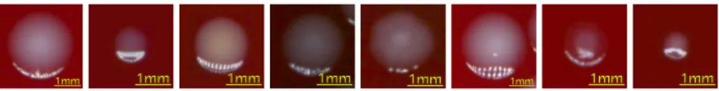
In Digital Microbiology Imaging (DMI), image-based decision making can be automated for certain tasks or support the work of the microbiologist for others. One of the most impacting capabilities (not yet provided by commercial prod-ucts) would be reliable and fast identification of bacterial species by direct image analysis and machine learning solutions. Early identification of bacteria species is needed to determine the correct therapy for the patient with potentially signifi-cant impact on life expectation. In addition, early identification is one of the most powerful ways to contrast the worldwide threat related to antibiotic resistance. This is especially true if one considers very general and massive diagnostic inves-tigation procedures such as screening for urinary tract infection (UTI) pathogen identification [13]. UTI are widespread and serious health problems that interest many millions of people every year around the world, accounting for a signifi-cant part of CM labs’ workload [14]. Unfortunately, presumptive identification by visual inspection of UTI pathogens on the most diffused culturing media (e.g. blood agar) can be a very complex and ambiguous task, even for highly skilled microbiologists (examples of different pathogens exhibiting high visual similarity are showcased in Fig. 1). This is the reason why, despite their higher cost, chromogenic media [15] have gained widespread market diffusion, thanks to their ability to mark different colonies with different colors (through the use of pathogen-specific enzyme substrates). However, these media have several
lim-Fig. 1: Examples of different UTI bacteria colonies grown on blood agar media.
itations in terms of the number of pathogens that can be differentiated [16]. HSI technology could provide support where three-chromatic imaging does not give enough spectral information for reliable discrimination. Therefore UTI identifi-cation is a good case study for HSI-based bacteria identifiidentifi-cation because UTI represents a diagnostic context involving, for a single laboratory, hundreds of analyses per day, so a technology investment can be rapidly amortized.
There are still very few examples of DL-based approaches for RS appli-cations [17–20] and, to our knowledge, still none for other fields, including biomedicine. Moreover, though both conventional machine learning [21–23] and DL solutions [24] have already been implemented for DMI analysis tasks, and hy-perspectral classification has already been explored in CM [25–29], the present work is the first attempt to combine HSI, CM-FLA and CNN for direct bacterial identification purposes. In this work, we want to exploit the enhanced spectral information coming from HSI acquisitions to prove the feasibility of reliable bac-teria species discrimination based on a DL approach. We raise the complexity of the problem compared to our preliminary study [27] by increasing the cardinality of pathogens, building a larger HSI UTI dataset (made available online) and by exploiting an improved acquisition setup. Unlike typical Remote Sensing tech-niques, that seek to increase the spatial consistency of the spectral classification at a pixel level [30], our pathogen recognition takes place on each single bacte-rial colony growing on the agar substrate. To this end, we propose a new (with respect to [27]) spatial-spectral distance measure to extract Colony Spectral Sig-natures (CSS). We designed and trained a 1D-CNN acting on CSS for pathogen identification and compared it against other conventional machine learning ap-proaches, well selected and designed for the same purpose [29]. In particular, classification accuracy, computational efficiency and scalability comparisons are proposed along with examples and further considerations.
2
Proposed Method
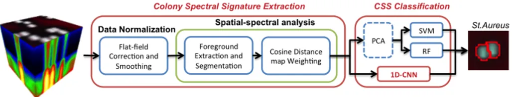
A general scheme of the proposed HSI processing and classification workflow for rapid UTI bacteria discrimination is given in Fig. 2. In describing the various stages of our system, we give more emphasis on the novel CNN-based solution for CSS discrimination. Details about other parts, HSI database and conventional handcrafted feature-based classification solutions can be found in [29].
Fig. 2: Processing and classification pipeline.
Hyperspectral Acquisition System The HSI target is a 90mm diameter Petri plate. The main parts of the acquisition system are: 1) HSI camera – a linear VNIR camera (Specim Spectral Camera V10E) with spectral range between 400 and 1000nm, tele-centric fore lenses (Specim OLE23, focal length 23mm); spatial resolution has been doubled with respect to [27] (640x600 pixels) maintaining scanning time under 15 seconds (compatible with FLA needs). 2) Illumination system – the light of two 150W halogen lamps is conducted by two 13mm-diameter optical fibers, spread by cylindrical lenses and finally reflected to the inner side of a semi-cylindrical dome. This configuration avoids total reflection effects on translucent colonies. 3) Conveyor system – a conveyor sliding system, mounting a shuttle which accommodates both the plate and a calibration bar (coated with BaSO4 optopolymer), allows push-broom plate acquisition and a
per-sample radiometric calibration.
Colony Spectral Signature (CSS) Extraction Flat-field calibration was applied to the hypercube to derive a normalized (with respect to a white calibration bar) relative reflectance measure Ri,λ
Ri,λ=
Si,λ− Di,λ
Wi,λ− Di,λ
(1)
where Si,λ is the acquired reflectance, Wi,λ and Di,λ are the white calibration
and the dark current spatial(i)-spectral(λ) profiles. A signal preserving Savitzky-Golay [31] denoising (window size of 7) is then applied. Since illumination power from the halogen sources decreases at the spectrum extrema, corresponding bands were cut off, preserving the ones with highest SNR in the range from 430nm to 780nm (for a total of 125 spectral bands). Then, a threshold-based foreground extraction is performed on the spectral band at wavelength 520nm. This produces a reliable isolation of the grown colonies because, at this specific wavelength, the contrast between relative reflectances of pathogens and blood agar is greater than in other bands. At this point, spatial distance transform is calculated for each colony using a spectral cosine distance map, computed as:
1 − u · v
||u||2||v||2, (2)
between each pixel signature v and the agar footprint u, obtained by averaging the spectral signatures of background pixels. We use the resultant map as an
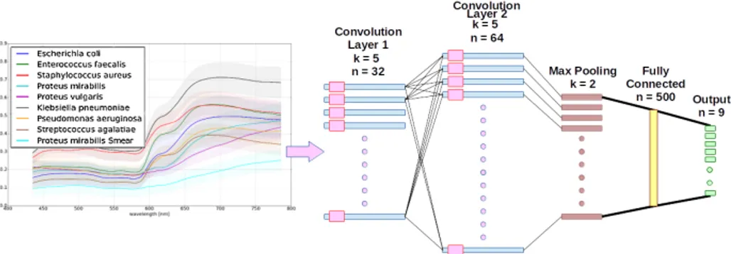
Fig. 3: Average spectral signatures of UTI bacteria, their standard deviations and CNN structure selected.
elevation map for a reliable watershed segmentation of bacterial colonies. For each detected colony we then extract a representative spectral signature (a 125-dimension vector) where we set colony pixel weighting factors proportional to the previously computed cosine distance map:
CSScolony=
X
p∈P
wp· Rp ∈ R125 (3)
with P the set of colony pixels, wp the weighting factor for the pixel p and Rp
the relative reflectance spectrum of the pixel p. Representative CSSs for each pathogen (the list is given in Sec.3) are shown in Fig. 3 (left), along with their standard deviation (shadowed).
Classification Methods CNN architectures [1] have been related to models of the visual cortex [32] and are characterized by locally overlapped connections (recep-tive fields) and shared weights implemented within a stacked hierarchy (from low to high level visual tasks) of convolutional feature extraction layers alternated with pooling layers (usually exploiting a max pooling rule). This is followed by one or more fully connected classification layers. Non-linear activation function layers are typically employed following convolutional ones, and the whole net-work produces a differentiable score function allowing the netnet-work parameters to be learned (weights and biases of the convolutional and fully connected layers). Unlike spatial-spectral 3D-CNN configurations [33], which are more suscepti-ble to overfitting and therefore needing dedicated regularization strategies, we exploit a 1D-CNN configuration similar to that considered in [33, 34] for RS hy-percubes. However, instead of considering single pixel spectra, we take advantage of the proposed spatial-spectral processing so that the CNN sees the extracted CSS as inputs while producing the colony-based class scores as output. Our network topology, see Fig. 3 (right), contains 2 convolutional layers, 1 pooling layer, 1 fully-connected layer and a final probability-based (softmax) classifier layer, for a total of 1,905,496 network parameters to learn. The first convolu-tional layer evaluates 32 feature maps from the 125-dimensional CSS input, for
each map a 5-tap filter is trained to produce same size output. The structure of the second convolution layer is similar and is composed of 64 feature maps (again 5-tap filters). Parametric Rectified Linear Units (PReLU) were used as activation functions [35]. After the two convolutional layers, a max pooling layer halves the size of feature maps given as input of a fully connected layer composed of 500 units, eventually followed by 9 output units. The selection of the above CNN structure was based on the evaluation of many possibilities by changing the number of convolutional and fully connected layers, learning rate and learning decay value (see Sec.3). We implement the whole structure in Python 2.7 and TensorFlow 1.0 [36].
For comparison purposes we selected two conventional classification approaches among those which have been shown to be effective in handling reflectance spec-tral data in this and other HSI analysis contexts: SVM and Random Forests. Support Vector Machine (SVM) [37] is a popular non-parametric technique for binary classification. It is a suitable tool in cases of data not regularly distributed or data with an unknown distribution. We implement SVM according to multi-class one-against-all structure, with Radial Basis Function kernels configured through iterated model selection for each pathogen binary classifier.
Random Forests (RF) [38] is an ensemble learning method that operates by constructing a multitude of decision trees. They predict (through a bagging ap-proach) deep insights into the structure of data. Each tree is built on different samples with randomness in the growing phase to ensure dissimilarity. Class with most votes (among all the trees in the forest) determines the prediction. The use of randomness and averaging improves the predictive accuracy and con-trasts overfitting. We also tested both SVM and RF combined with information preserving dimensionality reduction obtained by Principal Component Analysis (PCA) [39], used to reduce spectral redundancy with 99.9% of retained variance.
3
Results and Discussion
We built and analyzed a database of 16642 colonies streaked and grown on Petri dishes (5% sheep blood agar plates, BBL, BD Diagnostics, Sparks, MD) from 106 HSI volumes acquired after 18 hours of incubation in O2. Target
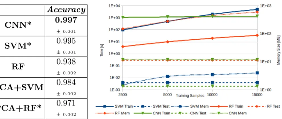
pathogens in our analysis, all belonging to the American Type Culture Collec-tion (ATCC), and covering over 85% of UTI species of interest, are: E.coli (5539 colonies), E.faecalis (1958), S.aureus (2355), P.mirabilis (2315), P.vulgaris (654), K.pneumoniae (542), Ps.aeruginosa (1529) and Str.agalactiae (1750). Represen-tative colony examples (from RGB images) and corresponding average spectral signatures are shown in Fig. 1 and Fig. 3 respectively. The whole dataset has been licensed for research use and can be accessed on http://www.microbia.org. Classification accuracy Bacterial species classifiers based on CNN, as well as SVM and RF (with or w/o PCA) have been implemented and compared on the experimental dataset. In Table 1, classification performance in terms of average accuracy are reported.
Accuracy CNN* 0.997 ± 0.001 SVM* 0.995 ± 0.001 RF 0.938 ± 0.002 PCA+SVM 0.984 ± 0.002 PCA+RF* 0.971 ± 0.002 Table 1: Classification accuracy (avg and std). With asterisk configura-tions considered in Fig. 4.
Fig. 4: Computational and memory footprint perfor-mance: training times–solid line, testing times –dashed line, and memory footprint–dotted line of the classifiers, versus the number of training samples
The selected CNN model, after 50,000 training iterations, reached an accu-racy of 99.7% becoming our best option. A learning rate of 0.01 and learning decay of 0.005 were selected after many different tests, resulting in the follow-ing observations: a) by growfollow-ing the number of convolutional and/or FC layers we obtained minor improvements with more than double the training/testing time; b) comparable classification results can be obtained with learning rates between 0.005 and 0.01, while using 0.05 leads to a lack of convergence for all tested configurations except a suboptimal one with single Conv and FC layers; c) with dropout of 0.75 and momentum of 0.9 (commonly adopted values) we preserve both the network structure and highest accuracy levels with training and test timings fully acceptable to guarantee FLA compatible near real-time classification (see below).
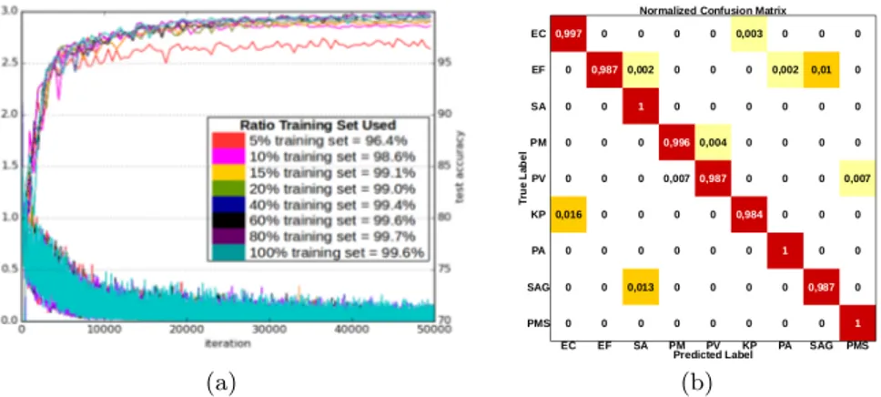
Accuracy assessments are based on a 70/30 random split in training and validation sets for each class in the database and repeated five times following a Shuffle & Split cross-validation approach. For the CNN solution it is particularly significant to assess how the method behaves as the dimension of the training set decreases. We therefore considered different percentages of the training set and, in Fig. 5(a) we track accuracy performance as a function of the number of learning iterations. Several curves are used to show increased accuracy when increasing the training set dimension (we are able to reach accuracy already greater than 99% by using only 15% of the training set).
Though slightly inferior with respect to CNN, SVM also reached comparable performance, showing an accuracy peak of 99.5% without PCA, while we ob-tained > 1% accuracy drop by adopting dimensionality reduction. It is therefore possible to create hyper-surfaces (thanks to RBF kernels) to accurately separate the analyzed classes.
RF was used differently to normal. When making predictions on the test dataset, we tried to exploit every tree in the forest in order to leverage the full forest and benefit from averaging the prediction. A decision is taken only if
(a) (b)
Fig. 5: (a) CNN dataset evaluation and (b) Confusion matrix with 99.7% accuracy.
70% of the forest agrees. This may decrease the overall accuracy but it increases classification precision, and reduces wrong predictions for test samples that bring new factors that were not in the training set (as not yet considered species or other undesirable alterations). Using this configuration, RF obtains its own best performance using PCA (97.1%, i.e. +3.3pp with respect to the baseline). Computational and scalability assessment Fast CSS classification is needed espe-cially in the context of FLA. Classifiers present strong discrepancies in terms of computational efficiency and scalability features according to the dataset dimen-sion. This section analyses training time (Fig. 4 solid line), testing time (Fig. 4 dashed line) and classifier memory footprint (Fig. 4 dotted lined) versus the number of training samples. We used a standard PC for all classifiers (Intel Core i5-3470 CPU 4x3.2GHz, 16 GB RAM) except CNN (Intel Core i7-5930K CPU 12x3.5 GHz, 32 GB RAM, GeForce GTX TITAN X). SVM and CNN are the slowest proposed solutions by almost two order of magnitude as long as RF on training times. SVM has a bigger slope compared to CNN that maintains similar values throughout the dataset size (meaning a better scalability). RF generates many decision trees (1000 in configurations applied to our dataset) and in order to reduce the training time it is possible to prune some branches (or to limit the branching depth) in a possible trade-off with the accuracy. The cardinality of the dataset has little influence on the classification (testing) time. RF is the slowest (while CNN is the fastest) because any sample must flow along every decision tree. Classifier memory footprint rises for SVM and RF and it remains constant for CNN. In absolute, RF requires much more space than CNN and SVM. Though not the best in terms of accuracy, RF demonstrates a high level of precision (low false positives) and facilitates extrapolation of additional infor-mation. On the other hand, SVM shows great accuracy. CNN proved to be the best solution in terms of accuracy, memory footprint and testing time, as well as scalability with respect to the dataset dimension, while training time can be limited by using GPU and specific hardware.
Considerations and future directions Figure 5(b) shows the confusion matrix for the best CNN configuration. We observe only a few mutual misclassifications between Ent. faecalis and Str. agalact., Esch. coli and Kleb. pneum., couples of pathogens that produce colonies which are hardly distinguishable visually. They are also roughly spectrally similar (though in average separated by a bias term, see Fig.5). Noticeably, very few misclassifications exist between Proteus vulg. and the not swarming Proteus mirab. (also almost impossible to discriminate visually) while, in a previous work [27], these classes were not distinctly sepa-rated, so they were considered as joined. Discrimination capability between two species of the same bacterial genus, as for Proteus, is of high application value and this is evidence of the improved CSS extraction introduced in this work.
According to accuracy of classification, complexity of the structure, memory footprint, training and testing times, the CNN-based method is seen as the best analyzed bacterial identification pipeline. However, near perfect species differen-tiation reveal the need and opportunities to further increase the number of con-sidered pathogens as well as the size and variability of the dataset (e.g. including plates coming from clinical specimens). Even if, on same experimental setting, conventional classification methods reached high classification performance as well, we can expect that DL-based approaches will be more appropriate in pres-ence of scalability needs and variability factors that will be considered in order to bring this HSI technology closer to clinical application.
4
Conclusion
We verified the possibility of applying a deep learning approach to UTI bacteria identification by using HSI technology operating in the VNIR spectrum. Our CNN-based solution obtained highest classification accuracies on a large labora-tory dataset, notwithstanding the significant number of analyzed pathogens and the fact that pathogen spectral signature differentiation is challenging and made even harder by spectral mixing with the growing media. There are also notable differences in term of scalability (both training, testing and memory used) driv-ing our CNN implementation selection above alternate methods. Improvements over previous works have also been obtained thanks to a better data acquisition setup and a more reliable CSS assessment. This study suggests that further in-vestigations are desirable by making our deep learning pipeline functional in a real clinical lab environment. Future activities should take into account an even higher number of UTI-relevant pathogens and clinical laboratory validations.
Acknowledgments
This work was partially supported by Italian Ministry of University and Re-search: Smart Factory Cluster, Adaptive Manufacturing, CTN01 00163 216730. The authors would to express their sincere thanks to the scientific and technical staff of Copan Group S.p.A. (Brescia, Italy) for their essential support in the creation of the hyperspectral image database.
References
1. LeCun, Y., Bengio, L., Haffner, P.: Gradient-based learning applied to document recognition. Proc. IEEE 86(11) (1998) 2778–2324
2. Litjens, G., Kooi, T., Bejnordi, B.E., Setio, A.A.A., Ciompi, F., Ghafoorian, M., van der Laak, J.A., van Ginneken, B., S´anchez, C.I.: A survey on deep learning in medical image analysis. arXiv preprint arXiv:1702.05747 (2017)
3. Serranti, S., Cesare, D., Marini, F., Bonifazi, G.: Classification of oat and groat kernels using nir hyperspectral imaging. Talanta 103 (2013) 276–284
4. Gowen, A., Feng, Y., Gaston, E., Valdramidis, V.: Recent applications of hyper-spectral imaging in microbiology. Talanta 137 (2015) 43–54
5. Liang, H.: Advances in multispectral and hyperspectral imaging for archaeology and art conservation. Appl. Physics A 106(2) (2012) 309–323
6. Lu, G., Fei, B.: Medical hyperspectral imaging: a review. Jour. of Biomed. Optics 19(1) (2014)
7. Wug Oh, S., Brown, M.S., Pollefeys, M., Joo Kim, S.: Do it yourself hyperspectral imaging with everyday digital cameras. In: IEEE CVPR. (2016)
8. Lambrechts, A., Gonzalez, P., Geelen, B., Soussan, P., Tack, K., Jayapala, M.: A CMOS-compatible, integrated approach to hyper- and multispectral imaging. In: IEEE Int. Electron Devices Meeting. (2014) 10.5.1–10.5.4
9. Bourbeau, P., Ledeboer, N.: Automation in clinical microbiology. Jour. of Clin. Microbiol. 51(6) (2013) 1658–1665
10. Novak, S., Marlowe, E.: Automation in the clinical microbiology laboratory. Clinics in Lab. Medicine 33(3) (2013) 567 – 588
11. Rhoads, D., Sintchenko, V., Rauch, C., Pantanowitz, L.: Clinical microbiology informatics. Clin. Microbiol. Rev. 27(4) (2014) 1025–1047
12. Doern, C.D., Holfelder, M.: Automation and design of the clinical microbiology laboratory. In: Manual of Clinical Microbiology, Eleventh Edition. American So-ciety of Microbiology (2015) 44–53
13. Flores-Mireles, A.L., Walker, J.N., Caparon, M., Hultgren, S.J.: Urinary tract infections: epidemiology, mechanisms of infection and treatment options. Nature reviews. Microbiology 13(5) (2015) 269–84
14. Wilson, M.L., Gaido, L.: Laboratory diagnosis of urinary tract infections in adult patients. Clinical Infectious Dis. 38(8) (2004) 1150–1158
15. D’Souza, H., Campbell, M., Baron, E.: Practical bench comparison of BBL chro-magar orientation and standard two-plate media for urine cultures. Jour. Clin. Microb. 42(1) (2004) 60–64
16. Perry, J., Freydire, A.: The application of chromogenic media in clinical microbi-ology. Jour. of Applied Microbiol. 103(6) (2007) 2046–2055
17. Chen, Y., Zhao, X., Jia, X.: Spectral-spatial classification of hyperspectral data based on deep belief network. IEEE J. Sel. Topics Appl. Earth Observ. in Remote Sens. 8(6) (2015) 2381–2392
18. Makantasis, K., Karantzalos, K., Doulamis, A., Doulamis, N.: Deep supervised learning for hyperspectral data classification through convolutional neural net-works. In: 2015 IEEE IGARSS. (2015) 4959–4962
19. Zhang, L., Zhang, L., Du, B.: Deep learning for remote sensing data: A technical tutorial on the state of the art. IEEE Geosci. Remote Sens. Mag. 4(2) (2016) 22–40 20. Ma, X., Wang, H., Geng, J., Wang, J.: Hyperspectral image classification with small training set by deep network and relative distance prior. In: 2016 IEEE IGARSS. (2016) 3282–3285
21. Ferrari, A., Signoroni, A.: Multistage classification for bacterial colonies recognition on solid agar images. In: Imaging Systems and Techniques (IST), 2014 IEEE International Conference on, IEEE (2014) 101–106
22. Ferrari, A., Lombardi, S., Signoroni, A.: Bacterial colony counting by convolutional neural networks. In: 2015 37th Annual International Conference of the IEEE En-gineering in Medicine and Biology Society (EMBC). (2015) 7458–7461
23. Andreini, P., Bonechi, S., Bianchini, M., Mecocci, A., Di Massa, V. In: Auto-matic Image Analysis and Classification for Urinary Bacteria Infection Screening. Springer International Publishing, Cham (2015) 635–646
24. Ferrari, A., Lombardi, S., Signoroni, A.: Bacterial colony counting with convolu-tional neural networks in digital microbiology imaging. Pattern Recognition 61 (2017) 629 – 640
25. Yoon, S., Lawrence, K., Park, B.: Automatic counting and classification of bacterial colonies using hyperspectral imaging. Food and Bio. Tech. 8(10) (2015) 2047–2065 26. Leroux, D., Midahuen, R., Perrin, G., Pescatore, J., Imbaud, P.: Hyperspectral imaging applied to microbial categorization in an automated microbiology work-flow. In: Clinical and Biomedical Spectroscopy and Imaging IV. Volume 9537., SPIE (2015) 1–9
27. Turra, G., Conti, N., Signoroni, A.: Hyperspectral image acquisition and analysis of cultured bacteria for the discrimination of urinary tract infections. In: Engineering in Medicine and Biology Society, EMBC, IEEE (2015) 759–762
28. Kammies, T.et al..: Differentiation of foodborne bacteria using nir hyperspectral imaging and multivariate data analysis. Appl. Microb. Biotech. (2016) 9305–9320 29. Arrigoni, S., Turra, G., Signoroni, A.: Hyperspectral image analysis for rapid and accurate discrimination of bacterial infections: a benchmark study. Computers in Biology and Medicine (2017) accepted paper.
30. Bernard, K., Tarabalka, Y., Angulo, J., Chanussot, J., Benediktsson, J.A.: Spectral-spatial classification of hyperspectral data based on a stochastic minimum spanning forest approach. IEEE Trans. Image Process. 21(4) (2012) 2008–2021 31. Savitzky, A., Golay, M.: Smoothing and differentiation of data by simplified least
squares procedures. Analytical Chem. 36(8) (1964) 1627–1639
32. LeCun, Y., Bengio, Y., Hinton, G.: Deep learning. Nature 521(7553) (2015) 436– 444
33. Chen, Y., Jiang, H., Li, C., Jia, X., Ghamisi, P.: Deep feature extraction and clas-sification of hyperspectral images based on convolutional neural networks. IEEE Trans. Geosci. Remote Sens. 54(10) (2016) 6232–6251
34. Li, J., Bruzzone, L., Liu, S.: Deep feature representation for hyperspectral im-age classification. In: 2015 IEEE International Geoscience and Remote Sensing Symposium (IGARSS). (2015) 4951–4954
35. He, K., Zhang, X., Ren, S., Sun, J.: Delving Deep into Rectifiers: Surpassing Human-Level Performance on ImageNet Classification. ArXiv e-prints (2015) 36. Abadi, M.et al..: Tensorflow: A system for large-scale machine learning. In:
Pro-ceedings of the 12th USENIX Conference on OSDI’16. (2016) 265–283
37. Cortes, C., Vapnik, V.: Support-vector networks. Machine Learning 20(3) (1995) 273–297
38. Breiman, L.: Random forests. Machine Learning 45(1) (2001) 5–32
39. Shaw, G., Manolakis, D.: Signal processing for hyperspectral image exploitation. IEEE Signal Process. Mag. 19(1) (2002) 12–16