The effect of economic crisis on regional income inequality in Italy

Università Cattolica del Sacro Cuore

DIPARTIMENTO DI SCIENZE ECONOMICHE E SOCIALI

The effect of economic crisis on regional

income inequality in Italy

Chiara Mussida

Maria Laura Parisi

Quaderno n. 114/luglio 2016

V

P_________

U N I V E R S I T À



Assistant Professor, Department of Economic and Social Sciences,

Università Cattolica del Sacro Cuore, e-mail:

chiara.mussida@unicatt.it

 _{Corresponding author: Associate Professor of Economics,}

Department of Economics and Management, University of Brescia, via San Faustino 74/b, Brescia, tel.: +39 030298 8826, email: marialaura.parisi@unibs.it

2

Chiara Mussida, Dipartimento di Scienze Economiche e Sociali, Università Cattolica del Sacro Cuore, Piacenza Maria Laura Parisi, Università degli Studi di Brescia

 chiara.mussida@unicatt.it

 marialaura.parisi@unibs.it

I quaderni possono essere richiesti a:

Dipartimento di Scienze Economiche e Sociali, Università Cattolica del Sacro Cuore

Via Emilia Parmense 84 – 29122 Piacenza – Tel. 0523-599.342

 dises-pc@unicatt.it

All rights reserved. Photocopies for personal use of the reader, not exceeding 15% of each volume, may be made under the payment of a copying fee to the SIAE, in accordance with the provisions of the law n. 633 of 22 april 1941 (art. 68, par. 4 and 5). Reproductions which are not intended for personal use may be only made with the written permission of CLEARedi, Centro Licenze e Autorizzazioni per le

Riproduzioni Editoriali, Corso di Porta Romana 108, 20122 Milano, e-mail: autorizzazioni@clearedi.org, web site www.clearedi.org.

Le fotocopie per uso personale del lettore possono essere effettuate nei limiti del 15% di ciascun volume dietro pagamento alla SIAE del compenso previsto dall’art. 68, commi 4 e 5, della legge 22 aprile 1941 n. 633.

Le fotocopie effettuate per finalità di carattere professionale, economico o commerciale o comunque per uso diverso da quello personale possono essere effettuate a seguito di specifica autorizzazione rilasciata da CLEARedi, Centro Licenze e Autorizzazioni per le Riproduzioni Editoriali, Corso di Porta Romana 108, 20122 Milano, e-mail: autorizzazioni@clearedi.org e sito web www.clearedi.org.

3

Abstract

This paper analyzes the determinants of unequal income distribution across macro-regions in Italy, and whether the latest economic crisis has had an effect on income inequality within or between regions. Inequality between individuals and between families appears greatest in the south, and the crisis has exacerbated this phenomenon. Econometric analyses by population groups and by nationality suggest that high educational attainment levels and larger households contribute to increasing the household income, whereas being female

and foreign tend to reduce household income. The

income distribution of foreign-born individuals tends to be more asymmetric, with heavier tails, compared to that of nationals.

JEL Classification codes:

Keywords:

5

1.Introduction

Regions are the destinations of individual workers, including migrants with foreign nationality, who choose their final destination by work opportunities, education, health or family reasons. This work analyses income unequal distribution across macro-regions in Italy.1 In particular, the individual and household characteristics affecting income inequality (age, gender, skill or education, employment status, household size and composition) across regions are identified. An important issue is whether the latest economic crisis has changed income inequality within or between regions of Italy. These issues are addressed by comparing two waves of EUSILC data in 2009 and 2014, representative of national residents (only), and by using ISTAT 2009 CVS data, to include foreign-born residents.

Although 16 years have passed since the Euro-zone was born with the primary objective of economic convergence across

1 _{Macro regions of Italy are the North West (Lombardy, Piemonte,}

Liguria, Valle d’Aosta), North East (Trentino-Alto Adige, Veneto, Emilia Romagna, Friuli Venezia Giulia), Centre (Lazio, Tuscany, Marche, Umbria), and South (Campania, Puglia, Abruzzo, Molise, Calabria, Basilicata, Sicily, Sardinia). EUSILC database collects information about residency at the macro-regional level NUTS-1, which divides Italy into 5 macro areas (South and Islands are aggregated).

6

states, the Eurostat Regional Yearbook in 2010 confirmed that considerable disparities still exist between the EU regions. Italy is a good starting point of analysis, since there are considerable regional growth disparities also within the country, i.e., across regions. There are indeed structural regional inequalities in the distribution of income across Italian macro-regions. Moreover, over the past 10 years Italy has increasingly become a destination country for a large number of foreigners/immigrants for economic reasons (Venturini and Villosio, 2006), who might have contributed to change the regional income distribution.2 As for other developed countries, this demographic change raises questions with respect to social inclusion, integration, cohesion and the extent of inequalities at both social and economic levels. These issues are quite important and currently highly debated, since they raise concerns for the policy makers.

The extensive literature existing on regional income inequality focused mostly on the historical causes, economic structures,

2

According to the Annuario Statistico Italiano (ISTAT, 2015) 60% of the 598,567 foreigners entering the country in 2010 had a work permit, while 30% entered for family reasons. In 2014, interestingly, only 23% of the 248,323 foreigners entered Italy for work reasons while 41% for family reasons. The rest of immigration permits generally relates to education, political asylum and humanitarian requests, religious, residency and health reasons.

7

economic growth, national market integration and regional convergence (one recent overview and reference is for example Tirado, Diez-Minguela, and Martìnez-Galarraga (2015), who use spatial autocorrelation regressions, inequality and mobility indexes for Spain over a long time period). In this work, the spirit of Cerqueti and Ausloos (2015) and Jenkins (1999) is followed to derive a plethora of indexes of regional income inequality, based on the ‘equivalised-household income’:3 Gini, the General Entropy class, the Atkinson class, the Palma index and few other percentile-ratios. The entire income distribution and its most relevant features, in terms of symmetry and tail-thickness, are also analysed. Significant differences in these features as well as in the inequality indexes are tested between year 2009 and 2014. The 2009 database allows measuring inequality and skewness in the pre-crisis period, while the 2014 database allows evaluating whether the economic crisis contributed to accrue economic inequalities within or between Italian regions. Then, a MLE approach is used to estimate the impact of individual and household characteristics on the distributional features of the equivalised-household income in every Italian

3

See Data and Indicators section for a complete definition and sources.

8

region, distinguishing by type of nationality of individuals in the household.

The paper has the following structure: section 2 sketches the relevant literature. Section 3 describes the data and defines the indicators. Section 4 analyzes the shape of income distribution across the macro-regions. Few conclusions on the statistical differences of regional income features between 2009 and 2014 are drawn. Section 5 reports the MLE coefficients (semi-elasticities) of the equivalised-household income for the different samples of households. Section 6 concludes.

2. Literature review

The aim of the empirical analyses of this paper is to understand the determinants of (household) income unequal distribution41 across macro-regions in Italy and migration is one of the potential determinants. However, other studies emphasize the impact of (other) individual and household characteristics affecting income inequality. In this section the

4

In general, household income inequality in Italy is one of the highest in developed countries. At the end of the 1990s, income inequality in Austria, Finland, Germany, Norway, Slovenia and Sweden was more than one fifth lower compared to Italy (Atkinson and Brandolini, 2004; Brandolini and Smeeding, 2005).

9

main determinants of income inequality suggested by the literature are discussed.

As far as migration phenomenon is concerned, Italy over the past 10 years has increasingly become a destination country for a large number of immigrants especially for economic reasons (Venturini and Villosio, 2006), who might have contributed to change regional income distribution and inequality. In the last years, indeed, the increasing volume of migrants in Italy from more disadvantaged countries for economic reasons, among others, has generated discussion around the economic assimilation process of immigrants and the consequences of migrations (Reyneri, 2007).

The extensive literature on the impacts of migration tried to emphasize the impacts and the relevance of this phenomenon for its effects on the country of destination. As per Italy, the migration history was characterized by both the presence of a relevant international migration and the recover (after a period of not relevant internal migration flows) of internal migration flows especially from the South to the North of the country (e.g., Carillo, 2012). The regions of destination of the migrants were traditionally Northern regions, whereas especially recently also Southern regions are increasingly relevant for the potential presence of foreign and irregular work for migrants (Bettio et al., 2006). However, the

10

international (or external/from abroad) and the internal migration have significantly different implications/impacts on the economy as a whole. As opposite to internal migration, international/migrants from abroad are on average less educated and qualified compared to internal migrants and therefore do suffer of a lower level of social and economic inclusion (De Palo et al., 2006, and Faini et al., 2009). In general, the two different migration flows (internal versus external) might have at least two opposite impacts on the regional income and also on (average) human capital levels. On the one hand, the increasing migration might exacerbate the regional disparities both in terms of income (unequal distribution of income across macro-regions) and human capital, i.e., migrants are low skilled and poorer compared to non-migrants. On the other and opposite hand, instead, migrants might contribute to reduce the regional gaps by increasing the economic, human capital and, more in general, social conditions of the regions of destination. The literature tried to disentangle the predominant effect of migration, i.e., increasing or reducing inequality, and the results are mixed. As far as other individual and household characteristics affecting income inequality are concerned, in their work, Checchi and Peragine (2010) found that gender and region (geographical area of residence) are important determinants of

11

opportunity inequality in Italy. Their results suggest that inequality of opportunities is much higher in the South, especially for women. The analysis of the entire income distribution reveals that men and women from Southern regions tend to be overrepresented in the bottom part of the distribution, while the opposite occur to the other tail for Northern workers. Thus in Italy the inequality of opportunities generated by family origins takes different faces according to gender and geographical area of residence. A woman born and working in the South is the most discriminated in terms of opportunities, especially when ending up in the bottom of the earning distribution. Similarly a man born and working in the South experiences increasing inequality of opportunity when going to the top of the distribution. Gender and geographical area of residence, therefore, are two important factors affecting income inequality. While inequality of opportunity in the entire Italian population accounts for one third of overall income inequality, the less developed regions in the South characterized by greater disparities at the global level, suffer greater incidence of opportunity inequality when disaggregated by gender. Common to many other less developed regions, Southern Italian regions experience the worst of possible worlds: lower per-capita income, higher

12

unemployment rates accompanied by greater overall income inequality.

Education also exert an important role on equality of opportunity and consequently on inequality of income as well (Peragine, 2004). In detail, higher social origins including higher educational attainment levels, as explained above for migration flows, are positively associated to income (De Vogli et al. 2010) and to equality of opportunities (Checchi and Peragine, 2010). In addition, household characteristics, i.e., number of household members and the presence of children, importantly affect household income.

To sum up, in this work analyses the relevance of migration, together with individual characteristics, i.e., gender, geographical area of residence, age, education, marital status, and household characteristics, i.e., household size and presence of children, on household income inequality, which, as suggested in this brief review of the relevant literature, are potentially important determinants of (regional) income inequality in Italy.

In addition, the paper also examines whether the latest economic crisis has changed (household) income inequality especially within or between regions in Italy. In general, there is more evidence that financial crises are followed by rising

13

inequality (Atkinson and Morelli, 2011). This, as explained above, was the case of Italy at the beginning of the 1990s.

3. Data and indicators

The data used in this work come from the European Union Statistics on Income and Living Conditions (EU-SILC) survey for the household without immigrants and from the ad-hoc survey on households with foreign people (CVS-2009) conducted by the Italian National Institute of Statistics (ISTAT, 2011). EU-SILC is a rotating panel survey based on a harmonized methodology and definitions across most members of the European Union (see EUROSTAT, 2010, for further and technical details). The topics covered by the survey are living conditions, income, social exclusion, housing, work, demography, and education. Data for Italy are selected, where the survey is conducted on a yearly basis by ISTAT, under the coordination of Eurostat.

The rotation scheme of the EU-SILC reduces the risk of attrition, i.e., the unit non-response of eligible persons or households that occurs after the first wave of the panel (Rendtel, 2002). The sampled units (households) to be added each year and the whole sample in the first wave of the survey

14

are selected according to two-stage stratified sampling designs, i.e., municipalities and households.

The waves of households observed in 2009 and 2014 are selected for (at least) two reasons. First, EUSILC collects incomes registered in the year before by the national tax office. The year 2009 is chosen when, one confidently supposes, there had not been any evident effect of the crisis yet. Then these incomes are compared with those collected in 2014 (produced in 2013), when the crisis bites already hit the ground. The second reason is that EUSILC-2009 provides incomes of the group of national residents, to compare to those of CVS-2009.

The data on the households with foreign members come from the Survey on Income and Living Conditions of Household with Foreign People conducted in 2009 by the Italian Statistical Institute (CVS-2009). The survey covers a larger sample of foreign households than the national EU-SILC. The two surveys share the same methodology and definitions, which allow us to use both in order to compare living conditions of native and foreign households.

The definition of equivalised-household income, the main variable of interest, is per capita income per household member weighted in proportion to the member’s needs. It is calculated dividing the household net income by the total of

15

the weights assigned to the people living in the household, based on their needs and based on the EU standards. The equivalised-household income is computed from the total disposable household income, variable HY020 in the EU-SILC code, applying the within-household non-response inflation factor, HY025, and the equivalised-household size, which gives each household member a specific weight.5 This income is deflated by using the Consumer Price Index (CPI), gathered by ISTAT.

The equivalised-household ln-income is the dependent variable of the econometric analyses described and commented in Section 5. The control variables include a dummy variable for marital status (married or not) and gender. Three different stages of education are considered and defined according to the International Standard Classification of Education (ISCED97): lower secondary education (ISCED97 levels 0–2), upper secondary education (ISCED97 levels 3 and

5 _{To reflect differences in a household's size and composition, the}

total net household income is divided by the number of 'equivalent adults’, using a standard equivalence scale, i.e., the modified OECD scale. In detail, this scale gives a weight to all members of the household (and then adds these up to arrive at the equivalised household size): 1.0 to the first adult; 0.5 to the second and each subsequent person aged 14 and over; 0.3 to each child aged under 14.

For additional details, see

16

4), and post-secondary or tertiary education (ISCED97 levels 5 and 6). Controls for individual age classes,6 household size, i.e., the number of household members, and for the number of children aged less than 16 in the household are also used. The general economic and labor market conditions are taken into account by including the unemployment rates by gender and region (ISTAT). Finally, a dummy variable for being a foreigner is considered into the set of explanatory variables.

4. The shape of household income distribution and the

economic crisis

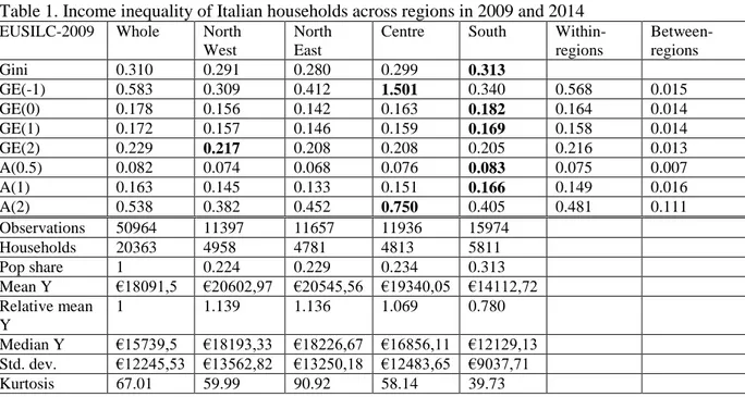
Table 1 reports few characteristics of income distribution of Italian households, calculated on EU-SILC 2009 (upper panel) and EU-SILC 2014 (bottom panel) income data for Italy (Whole), and separately by macro-region of residence. More than 50% of Italian population live in Centre-South of Italy (54.7%) according to EU-SILC data. This fact is confirmed by the population census figures (ISTAT, 2014).

The Northern regions are clearly better off than the rest. Household’s mean income in the North is above €20 thousand

6 _{Five age groups are considered in the estimates: [16-24] years old,}

17

per year compared to €14 thousand in the South. The average income of North Eastern households is 13% above the population average, the average income of North Western households is 14% above the population average while the average income of Southern households is about 22% below the population average. Description analysis is restricted to households with positive observed income. In 2014, there are 46,778 individuals with positive income, in 19,474 households, in the EU-SILC wave for Italy.

Table 1 reports also the inequality indexes. In general, higher index values are associated to higher inequality, and indexes vary for their level of sensitivity to portions of the income distribution, as well as whether they are additively decomposable into within and between-group inequality. The class of General Entropy indexes in Table 1, GE(a), includes a={-1, 0 (mean log-deviation), 1 (Theil), 2 (½ the square of coefficient of variation)}. As discussed above, a higher positive parameter a is associated to more sensitivity to income differences at the top of the distribution. Moreover, GE measures with a>1 are very sensitive to high incomes in the data (Cowell and Flachaire, 2007). The more negative a is, the more sensitive the index is to differences at the bottom of the distribution (and to small incomes). In the class of Atkinson indexes, A(e), e is an inequality ‘aversion’

18

parameter. Therefore, the more positive e the more sensitive A(e) is to differences at the bottom of the distribution. The Gini coefficient however is most sensitive to differences about the middle portion of the income distribution. One needs to be careful at taking extreme values of these parameters, as the presence of one or two very large or small outliers might influence the value of indexes.

In the upper panel, inequality appears greatest for Southern households compared to the others, especially for the middle portion-difference sensitive GE(0), GE(1), A(0.5), A(1) and Gini index. Households in the Centre regions appear to have highest inequality according to GE(-1) and A(2), i.e. the bottom-tail-difference sensitive indexes. Only GE(2), sensitive to top-income differences, indicates highest inequality within the North West macro-region.

In other words, in 2009 in the South, households and individuals had lower incomes and highest inequality. An exception is the highest share of income distribution in the North West, for which inequality was very high.

In the bottom panel, inequality indexes reveal again greatest inequality in the South, including GE(2), while the Centre households income produce greatest inequality values again according to GE(-1) and A(2), i.e. at the bottom tail, although the two indexes are now lower than in 2009. Indeed, it is

19

possible to compare the difference of all indexes over time through a t-test for significance as shown in Table 2. Before discussing the results of the tests, comments on the last two columns of Table 1, which show a general decomposition of the indexes into within-region and between-region inequality are provided. Within-region inequality accounts for very much more of total inequality than between-region does. This is particularly true for bottom-sensitive indices GE(-1) and A(2), i.e. for the bottom tail of income distribution. However, it is noticed that, according to the Atkinson index A(2), there is also a non-negligible amount of between-regions inequality (0.147) that is not evident in other parts of the Italian households’ income distribution. This result is extremely interesting because the Italian economy in general and, more specifically, the Italian labor market is structurally characterized by a ‘regional divide’: the Italian households living in the South on average enjoy less favorable economic conditions. Regional economic disparities and cultural differences are significantly high. Thus higher between-region inequality would have expected, yet the data do not give evidence to this phenomenon (apart from the less wealthy households).

Finally, the kurtosis of the distribution for total population and by region in both panels are reported. This parameter indicates

20

that the tails of the income distribution is fatter than normal. For total population and North West macro-region in 2014, it became even fatter, while in the same year, compared to 2009, in other regions, kurtosis parameter decreased. Symmetry and tails of income distribution over time are illustrated in Figure 1.

21

Table 1. Income inequality of Italian households across regions in 2009 and 2014

EUSILC-2009 Whole North

West

North East

Centre South

Within-regions Between-regions Gini 0.310 0.291 0.280 0.299 0.313 GE(-1) 0.583 0.309 0.412 1.501 0.340 0.568 0.015 GE(0) 0.178 0.156 0.142 0.163 0.182 0.164 0.014 GE(1) 0.172 0.157 0.146 0.159 0.169 0.158 0.014 GE(2) 0.229 0.217 0.208 0.208 0.205 0.216 0.013 A(0.5) 0.082 0.074 0.068 0.076 0.083 0.075 0.007 A(1) 0.163 0.145 0.133 0.151 0.166 0.149 0.016 A(2) 0.538 0.382 0.452 0.750 0.405 0.481 0.111 Observations 50964 11397 11657 11936 15974 Households 20363 4958 4781 4813 5811 Pop share 1 0.224 0.229 0.234 0.313 Mean Y €18091,5 €20602,97 €20545,56 €19340,05 €14112,72 Relative mean Y 1 1.139 1.136 1.069 0.780 Median Y €15739,5 €18193,33 €18226,67 €16856,11 €12129,13 Std. dev. €12245,53 €13562,82 €13250,18 €12483,65 €9037,71 Kurtosis 67.01 59.99 90.92 58.14 39.73

22

EUSILC-2014 Whole North

West

North East

Centre South

Within-regions Between-regions Gini 0.317 0.297 0.278 0.309 0.326 GE(-1) 0.757 0.478 0.231 1.413 0.745 0.742 0.015 GE(0) 0.195 0.166 0.141 0.181 0.216 0.181 0.014 GE(1) 0.179 0.159 0.142 0.169 0.187 0.165 0.014 GE(2) 0.227 0.209 0.189 0.210 0.227 0.213 0.013 A(0.5) 0.087 0.076 0.067 0.082 0.093 0.080 0.008 A(1) 0.177 0.153 0.131 0.165 0.194 0.162 0.019 A(2) 0.602 0.489 0.316 0.739 0.598 0.533 0.147 Observations 46778 11120 11315 11126 13217 Households 19474 4888 4716 4615 5255 Pop share 1 0.266 0.193 0.199 0.342 Census share§ 1 0.265 0.192 0.199 0.344 Mean Y €18139,4 €20716,85 €20464,61 €19366 €14113,23 Relative mean Y 1 1.142 1.128 1.068 0.778 Median Y €15946.7 €18050 €18395 €16960,8 €12247,78 Std. dev. €12214,7 €13406,14 €12570,44 €12554,4 €9504,63 Kurtosis 75.24 142.4 42.06 28.2 20.56

Note: Blue = increase in inequality index or kurtosis measure; Green = decrease in inequality index or kurtosis measure with respect to 2009. § ISTAT, Annuario Statistico Italiano: Population at 31 December 2014. South share is 0.233 and Islands share is 0.11. Source: Authors’ elaborations on EU SILC 2009 and EU SILC 2014 data.

23

Table 2 shows the Student’s t-tests - and their p-values - of the difference in values of all indexes between 2009 and 2014. The null hypothesis is . The asymptotic sampling variance for each index is used, as explained by Jenkins (1999), Biewen and Jenkins (2003). In particular, the variance formulas need to adjust to the effects of complex survey design features (stratification and clustering) of EU-SILC. In general, statistical significance arises towards increasing values, i.e. in 2014 some of the calculated indexes indicate increasing inequality. If one looks at total population, a significant increase, above 5%, according to Gini, GE(0), A(0.5) and A(1), is noticed, that means that inequality around the middle portion of income distribution arose. This is particularly true in the Centre and South of Italy. The North West experienced a significant increase in inequality according to A(2) index. The North East macro-region has not experienced any significant change in inequality.

24

Table 2. Test for statistical difference of inequality indexes between 2009 and 2014

EUSILC-2014 vs EUSILC- 2009

Whole North West North East Centre South

Gini ttest 1.730** 0.745 -0.281 1.386* 1.800** pvalue 0.042 0.228 0.611 0.083 0.036 GE(-1) ttest 0.575 1.186 -1.111 -0.056 2.446*** pvalue 0.283 0.118 0.867 0.522 0.007 GE(0) ttest 3.318*** 1.013 -0.212 1.847** 3.368*** pvalue 0.000 0.155 0.584 0.032 0.000 GE(1) ttest 1.265 1.013 -0.351 1.022 2.037** pvalue 0.103 0.155 0.637 0.153 0.021 GE(2) ttest -0.172 -0.625 -0.625 0.082 1.264 pvalue 0.568 0.734 0.734 0.468 0.103 A(0.5) ttest 2.279** 0.601 -0.236 1.559** 2.659*** pvalue 0.011 0.274 0.593 0.059 0.004 A(1) ttest 3.325*** 1.014 -0.212 1.849** 3.396*** pvalue 0.000 0.155 0.584 0.032 0.000 A(2) ttest 0.563 1.358* -1.357 -0.056 3.445*** pvalue 0.287 0.087 0.913 0.522 0.000

Note: * 10%, ** 5%, *** 1% significance levels.2-sided Student’s t-test of significance for the difference in 2009 and 2014. Positive significant value of the test means that the index has increased from 2009 to 2014, amplifying inequality over time, especially in the Centre-South of Italy. Source: Authors’ elaborations on EU SILC 2009 and EU SILC 2014 data.

25

The Centre experienced an increased inequality for middle incomes. The South, on the other hand, is the region where most of the indicators calculated show an increased inequality over time. This appears to happen almost in all deciles of the income distribution. The latest economic crisis tended to exacerbate economic inequality among individuals and their families in the South.

Nonparametric density for the level of equivalised-household income of Italian households – total population is estimated. First skewed-Normal distribution is estimated and compared to a skewed-Student’s t distribution, taking the parameters of symmetry and variance into account (see Marchenko and Genton, 2010, Azzalini and Genton, 2008). The ‘gamma’ and ‘alpha’ parameters of symmetry and ‘df’ parameter of heavy-tails are approximate indicators of income inequality. The estimated parameters of the income distribution by region and year are reported in Figure 1. The upper panel shows the symmetry parameter Gamma when the distribution with a skewed-Normal is estimated. A positive value of Gamma indicates asymmetry to the right (long-right tail). When Gamma = zero the distribution becomes symmetric (and the skewed-Normal density becomes Normal). In both years, Gamma is positive in all regions. It appears to be higher in the

26

North East and South in 2009, with a tendency to diminish in 2014. In the North West, Gamma becomes higher in 2014. In the middle panel, the parameter ‘Alpha’ of asymmetry in a skewed-Student’s t distribution is reported. If Alpha > 0, it indicates an asymmetry to the right. If Alpha = zero, the skewed-Student’s t reduces to the Student’s t. Alpha is positive in both years for all regions. It is highest for the South, but it becomes smaller in every region in 2014. Finally, in the bottom panel of Figure 1, the Heavy-tail DF index after estimating the skewed-Student’s t distribution are reported. The lower this parameter, the heavier the tails of the distribution. On the other hand, an infinite value of DF means that the skewed-t reduced to a skewed-Normal. The DF indicates that the tails of income distribution are quite fat in all regions and over time, with the northern regions having heavier tails. This might signal the fact that household income in those regions is less ‘unequal’ than in the Centre-South, as the analysis above reveals. These values plus a QQ-plot analysis suggests preference for a skewed-Student’s t density for the Italian equivalised-household income.

Finally, since the inequality indexes might be particularly sensitive to certain portion of the income distribution, as explained above, the income share differences between 2009 and 2014 by population percentages for both total population

27

and separately by each region are calculated. This allows studying the unequal distribution of income within quintiles. The Gini coefficient, for instance, is most sensitive to differences in the middle portion of the income distribution. By calculating the income shares at each quintile, one has the opportunity to understand where the changes of these shares were concentrated, or mostly affected by the crisis (Jahn, 2016). To address the sensitivity problems of the inequality indexes, the Palma ratio (Palma, 2011), defined as the ratio of the richest 10% of the population's share of gross national income divided by the poorest 40%'s share, is also calculated. It is based on the assumption that middle class incomes almost always represent about half of gross national income while the other half is split between the richest 10% and poorest 40%, but the share of those two groups varies considerably across countries. In detail, the Palma ratio addresses the Gini index's over-sensitivity to changes in the middle portion of the distribution and

28

Figure 1. Estimated parameters of Asymmetry and Kurtosis for equivalised-hh income distribution by region-time.

2009

2014

Gamma Index of Asymmetry

Alpha Index of Asymmetry

0.86 0.88 0.9 0.92 G a mma Sk e w n e s s i n d e x

North-West North-East Centre South

2009

Skewed-normal distributed equiv-income: Asymmetry

0.84 0.86 0.88 0.9 0.92 G a mma Sk e w n e s s i n d e x

North-West North-East Centre South

2014

29

Heavy-Tail DF Index

North-West North-East Centre South

2009

Skewed-t distributed equiv-income: Asymmetry

2 2.2 2.4 2.6 2.8 Al p h a S k e w n e s s i n d e x

North-West North-East Centre South

2014

30

Note: based on 50964 observations in 2009, 46864 observations in 2014.If gamma=0 the distribution is symmetric (it reduces to normal). If gamma>0 the distribution is skewed to the right. In both years, gamma is estimated different from zero in all macro-regions in Italy. If alpha=0 in the second panel, the distribution becomes the symmetric Student’s t. If alpha>0 it is skewed to the right. If df=∞ the skewed-t becomes the skewed-normal distribution: the lower df, the heavier the tails of the distribution. If alpha=0 and df=∞ the distribution becomes normal.

Source: Authors’ elaborations on EU SILC 2009 and EU SILC 2014 data. 3 3.5 4 4.5 D F H e a v y -t a il i n d e x

North-West North-East Centre South

2009

Skewed-t distributed equiv-income: Kurtosis

3 3.5 4 4.5 D F H e a v y -t a il i n d e x

North-West North-East Centre South

2014

31

insensitivity to changes at the top and bottom, therefore it more accurately reflects income inequality's economic impacts on society as a whole. The Palma ratio for Italy and by region confirms an increase in income inequality, especially in the South.7

7

For the sake of brevity, the values of the ratio are not reported. Nonetheless, those are available upon request.

32

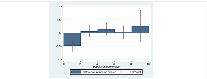
Figure 2. Income share differences between 2009 and 2014 by population percentages and regions

-1 0 1 -0.5 0.5 Pe rce n t 0 20 40 60 80 100 population percentage

33

Difference in Income Shares 95% CI

North West -1.5 -1 0 1 -0.5 0.5 Pe rce n t 0 20 40 60 80 100 population percentage

Difference in Income Shares 95% CI

34

Source: Authors’ elaboration on EU SILC 2009 and EU SILC 2014 data. -1 0 1 1.5 -0.5 0.5 Pe rce n t 0 20 40 60 80 100 population percentage

Difference in Income Shares 95% CI

Centre -2 -1 0 1 2 Pe rce n t 0 20 40 60 80 100 population percentage

Difference in Income Shares 95% CI

35

Figure 2 offers a detailed representation of the income share differences between 2009 and 2014 by population percentages (quintiles) for the overall population and for each region. It is an in-depth investigation of the changes in the distribution of income without any sensitivity problems. The top panel shows the income share differences for the total population. Income in Italy decreased in the first quintile of the distribution by around 0.5% whilst it increased in the fifth quintile by more than 0.25%. In the middle part of the distribution (from the second to the fourth quintile) changes were negligible (on average around 0.07%). By looking at the income share differences by region, the same behavior as for the overall country is found, i.e. reduction in the first quintile and increase in the fifth quintile between 2009 and 2014 everywhere, with the exception of the North East. The highest decrease in the first quintile happens in the South (around 0.9%) and in the Centre of Italy (around 0.6%) compared to the Northern regions, whereas the highest income increase at the top of the population distribution happens in the North-West (around 0.5%) and Centre. Summing up, these results suggest that the most relevant impacts of the crisis were concentrated in the first and bottom quintile, especially in Southern and Central regions. The income shares in the middle of the population

36

distribution, instead, were not significantly affected by the recession.

5. The shape of income distribution and household

characteristics: nationals vs foreigners

In this section, the impact of factors affecting the distribution of income is estimated. To distinguish whether migrants contributed to increase or reduce regional income inequality, the distribution of income for national and foreign-born households is estimated. The household/individual characteristics, which affect income inequality, include marriage status, gender, age, skill or education, employment status, household size and composition, region of residency, nationality. Given the cross-sectional features of the data used and the questions this work would like to answer, the following method to explore those issues here is adopted. The (log-) income is regressed by skewed-Student’s t MLE over the set of explanatory variables. The estimated parameters of asymmetry and heavy-tails are then registered, and the changes in these parameters are discussed as indicating more or less tendency to inequality across different groups (by nationality) and regions (see section 4 for a discussion on the

37

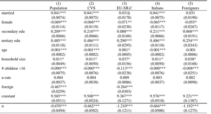
shape parameters). Skewness and heaviness of tails have of course a direct effect on inequality measures, e.g. percentiles or quintile ratios, such as the Palma ratio. For example, a heavy than Normal tail may increase the Palma ratio, ceteris paribus, indicating an increased income inequality in that population. Again, a high skewness to the left might increase the distance between median and mean income, with the latter lower than the former, pushing the Gini index towards 1. Table 3 reports the MLE coefficient estimates (semi-elasticity) for different samples. Column 1 refers to the entire population of CVS and EU SILC individuals. Column 2 relates to CVS individuals, who are mostly foreigners but with a group of Italians living in a household with at least one foreign-born component. Column 3 relates to EU SILC dataset, which collects data only for Italian nationals. Column 4 takes Italians from both sources (nationals + Italians in foreign households) and finally column 5 refers only to foreign-born people. For all groups but foreigners, being married is positively associated to a higher income. Female individuals have a negative coefficient estimate in all groups. The higher the share of female in the household, the lower its income. Being educated is important for sustaining household’s income, and having a tertiary degree is even more important. Age is slightly negatively correlated to income in total population, CVS and

38

Italians, it is slightly positively correlated in EU SILC (older nationals do have higher income on average) while it is not significantly important for foreigners. The number of household components (household size) seems to be positively correlated to income, but this is not so when households have little children at home (less than 16 years old). Employment status seems not to matter, but this is particularly related to little variation of the share of unemployed individuals in all groups. Being foreigner does not definitively help at sustaining income.

As far as the symmetry parameter alpha, it is negative and significant for all groups. This means that the distribution of ln-income is skewed to the left. The value of negative alpha is higher for the group EU SILC and Foreigners.

As far as the DF parameter, indicating heaviness of tails or kurtosis, when DF=∞ the distribution of income has the same tails as a Normal density. As a consequence, the lower DF the heavier the tails (and thus there is the need to adapt a Student t distribution). When df=∞ and α=0 then income is Normally distributed.

From the results obtained, it emerges that DF takes low values in all groups. The lowest values are those of Foreigners and EU SILC. From these first figures, it seems that Foreigners and national residents suffer from the highest within-group

39

inequality. The two groups are now compared disaggregating income distribution by region.

In Appendix, Figure A1 shows the kernel density estimation of income by region and nationality. Kernel density is calculated on the fitted values of income on the set of explaining variables. It is evident that the density of foreigners is more skewed, has heavier tails and it has lower range of values than that of national residents, especially in the Centre and South of Italy. The density of income of the nationals is smoother, with three or fewer modes.

Table 4 reports the regression results for ln-income in the four macro-regions and by nationality. When the results are disaggregated, few different and interesting conclusions can be drawn. Being married is not important for foreigners to sustain household income as much as for nationals, with an exception for Southern individuals. Secondary education seems to be important only for foreigners living in the Centre and South, while tertiary education is always positively associated to income. Household size becomes important for nationals only in the North East, while its coefficient is not significant in the rest of the regions. Household size looks important for foreigners, instead, apart from the North Western region. The share of unemployed individuals has a negative and significant impact only for nationals in the South.

40

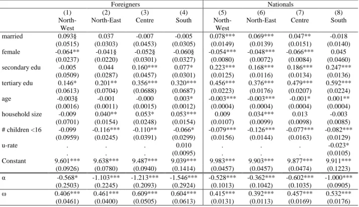
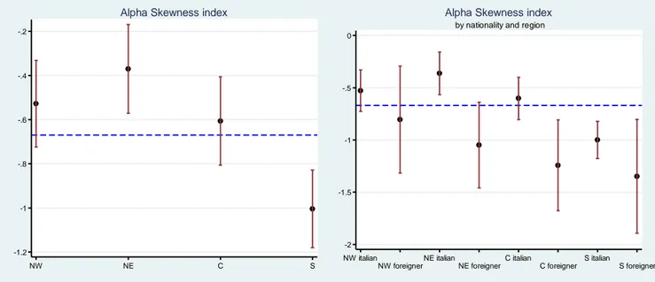
As far as the alpha parameter, there are differences across both regions and nationality. Foreigners’ income distribution appears to be more asymmetric in the Centre and South, and Foreigners do have a more skewed distribution than nationals within the same region too. See Figure A2 in Appendix. It is also true that Foreigners income distribution in the regions present heavier tails than the correspondent national distribution. See Figure A3 in Appendix.

It turns out that foreign incomes in the South are the most ‘unequally’ distributed among all groups.

The different variance within group is consistent to what other scholars found in their empirical research about ethnic groups experimenting mostly within-group inequality, much higher than Italian nationals (see for example D’Agostino, Regoli, Cornelio, and Berti, 2015). Nonetheless, the same group in different regions belong to quite a different income distribution, in terms of symmetry and kurtosis. This issue is explored in more detail in another work (Mussida and Parisi, 2016).

41

Table 3. Skew-Student’s t MLE of ln-Equivalised Income on different groups

(1) (2) (3) (4) (5)

Population CVS EU-SILC Italians Foreigners

married 0.041*** 0.041*** 0.031§ 0.041*** 0.031 (0.0074) (0.0075) (0.0178) (0.0075) (0.0190) female -0.069*** -0.068*** -0.071** -0.065*** -0.055* (0.0114) (0.0119) (0.0230) (0.0117) (0.0267) secondary edu 0.209*** 0.210*** 0.088*** 0.211*** 0.068*** (0.0066) (0.0066) (0.0160) (0.0066) (0.0191) tertiary edu 0.485*** 0.486*** 0.290*** 0.486*** 0.254*** (0.0110) (0.0111) (0.0295) (0.0110) (0.0343) age -0.001*** -0.001*** 0.001* -0.001*** -0.001 (0.0002) (0.0002) (0.0005) (0.0002) (0.0006) household size 0.011* 0.011* 0.037* 0.011* 0.038* (0.0049) (0.0050) (0.0156) (0.0050) (0.0168) # children <16 -0.090*** -0.090*** -0.113*** -0.090*** -0.098*** (0.0075) (0.0076) (0.0238) (0.0076) (0.0251) u-rate 0.004 0.004 0.009 0.003 0.002 (0.0037) (0.0038) (0.0086) (0.0037) (0.0098) foreign -0.467*** . -0.264*** (0.0259) . (0.0303) constant 9.565*** 9.568*** 9.367*** 9.576*** 9.221*** (0.0511) (0.0524) (0.1271) (0.0518) (0.1387) α -0.670*** -0.662*** -1.210*** -0.664*** -1.192*** (0.0494) (0.0502) (0.1211) (0.0500) (0.1275)

42

Standard errors in parentheses. § p < 0.10, * p < 0.05, ** p < 0.01, *** p < 0.001. Each column restrict the regression to the income of the indicated group. ‘Population’ is the CVS-EUSILC general database. ‘Italians’ include all Italian nationals in EUSILC and Italians in foreign households of CVS. ‘Foreigners’ include only foreign-born individuals from CVS. ‘Alpha’ is the index of asymmetry in income distribution. When α=0, the skew-t becomes Student’s t. When α<0 the asymmetry is on the left. ‘df’ is the parameter indicating heaviness of tails. When df=∞ the distribution has the same tails as a Normal density. The lower ‘df’, the heavier the tails of the distribution. When df=∞ and α=0 then the income is Normally distributed.

43

Table 4. Skew-Student’s t MLE of ln-equivalised income by nationality and region

Foreigners Nationals

(1) (2) (3) (4) (5) (6) (7) (8)

North-West

North-East Centre South North-West

North-East Centre South married 0.093§ 0.037 -0.007 -0.005 0.078*** 0.069*** 0.047** -0.018 (0.0515) (0.0303) (0.0453) (0.0305) (0.0149) (0.0139) (0.0151) (0.0140) female -0.064** -0.041§ -0.052§ -0.060§ -0.054*** -0.048*** -0.066*** 0.045 (0.0237) (0.0220) (0.0301) (0.0327) (0.0080) (0.0072) (0.0084) (0.0460) secondary edu -0.005 0.044 0.160*** 0.077* 0.223*** 0.168*** 0.186*** 0.247*** (0.0509) (0.0287) (0.0457) (0.0301) (0.0125) (0.0116) (0.0134) (0.0136) tertiary edu 0.146* 0.201** 0.356*** 0.320*** 0.456*** 0.376*** 0.479*** 0.592*** (0.0613) (0.0704) (0.0688) (0.0687) (0.0223) (0.0176) (0.0207) (0.0224) age -0.003§ -0.001 -0.000 0.003* -0.003*** -0.003*** -0.001* 0.001** (0.0016) (0.0011) (0.0015) (0.0012) (0.0004) (0.0004) (0.0004) (0.0004) household size -0.009 0.040** 0.053* 0.053*** 0.009 0.034*** 0.013 -0.003 (0.0701) (0.0154) (0.0248) (0.0154) (0.0107) (0.0099) (0.0098) (0.0085) # children <16 -0.099 -0.116*** -0.110** -0.066* -0.079*** -0.126*** -0.077*** -0.082*** (0.0959) (0.0245) (0.0391) (0.0299) (0.0156) (0.0144) (0.0163) (0.0129) u-rate . . . 0.010 . . . -0.023* . . . (0.0095) . . . (0.0105) Constant 9.601*** 9.638*** 9.487*** 9.039*** 9.983*** 9.903*** 9.877*** 9.911*** (0.0926) (0.0780) (0.0940) (0.1414) (0.0457) (0.0457) (0.0474) (0.1223) α -0.568* -1.103*** -1.213*** -1.546*** -0.528*** -0.362*** -0.602*** -1.000*** (0.2503) (0.2245) (0.2093) (0.2924) (0.1013) (0.1042) (0.1035) (0.0905) ω 0.406*** 0.461*** 0.609*** 0.604*** 0.415*** 0.392*** 0.457*** 0.532*** (0.0461) (0.0400) (0.0505) (0.0613) (0.0131) (0.0113) (0.0169) (0.0176)

44

df 2.969*** 2.873*** 2.840*** 2.473*** 4.127*** 4.443*** 4.686*** 4.716*** (0.4917) (0.3177) (0.3363) (0.3223) (0.2588) (0.3460) (0.3795) (0.2897)

Observations 2352 2539 2153 3697 12230 12556 12684 17386

Households 1171 1264 1117 2167 5379 5213 5194 6449

Standard errors in parentheses. § p < 0.10, * p < 0.05, ** p < 0.01, *** p < 0.001. Column (1) to (4) include dummies for ethnic groups. See note to Table 5.

45

6. Conclusions

This work analyzed the income unequal distribution across macro-regions in Italy. The data used allow examining whether income inequality changed after the economic recession.

The analysis of the shape of the income distribution suggests that Northern regions are better off than the rest of the country, both due to higher mean income and to lesser inequality. This is confirmed by a plethora of indexes of income inequality suggesting that inequality appears greatest for Southern households. In other words, households and individuals in the South have lower incomes compared to the other Italian regions and consequently highest income inequality. Inequality within regions makes most of total inequality than inequality between regions and the latest economic crisis tended to exacerbate economic inequality among individuals and their families in the South of Italy. These results are quite interesting for Italy, where regional economic and cultural differences are perceived to be quite high. Moreover, income reduction after the latest crisis intensified in the bottom portion of the income distribution, in the Centre and South.

The econometric investigation of the characteristics of the resident individuals and households affecting income inequality on different population groups and by nationality

46

(Italian or foreign) offer different and interesting conclusions. The analysis by population groups suggests that education and higher household sizes (without little children at home) contribute to increase the household (equivalised) income, whereas being female and foreign tends to reduce the income. For this and other reasons the issue of income inequality by nationality, i.e., for Italian and foreigners separately, have been investigated. Being married is not important for foreigners to sustain household income as much as for nationals. Secondary education seems to be important only for foreigners living in the Centre and South, while tertiary education is always positively associated to income. Household size looks more important for foreigners than nationals. The share of unemployed individuals has a negative and significant impact on household income only for nationals in the South.

The findings of this work therefore highlight the relevance of income inequality in Italy, especially since the recession and in the Southern regions of the country. In addition, foreigners are still disadvantaged even if migration is not a recent phenomenon in Italy. Policies to facilitate the access to highest educational levels especially for foreigners and to reconcile work and household duties especially for foreign females with young children might help reducing income inequality both

47

between foreigners and Italian nationals and between the South and the rest of the country.

48

References

Allasino, E., Reyneri, E., Venturini, A., & Zincone, G. (2004). Discrimination of Foreign Workers in the Italian Labour Market. International Migration Papers, 67, Geneva, ILO.

Atkinson, A.B., & Brandolini, A. (2004). I cambiamenti di lungo periodo nelle disuguaglianze di reddito nei paesi industrializzati. Rivista italiana degli economisti, 9, 389-421. doi: 10.1427/19762

Atkinson, A.B., & Morelli., S. (2011). Economic crises and Inequality, Human Development Research Paper, 2011/06.

Azzalini, A., & Genton, M.G. (2008). Robust likelihood methods based on the skew-t and related distributions. International Statistical Review, 76, 106-129. doi: 10.1111/j.1751-5823.2007.00016.x

Bettio, F., Simonazzi, A., & Villa, P. (2006). Change in care regimes and female migration: the ‘care drain’ in the Mediterranean. Journal of European Social Policy, 16(3): 271-285. doi: 10.1177/0958928706065598 Biewen, M., & Jenkins, S. P. (2003). Estimation of

Generalized Entropy and Atkinson indices from complex survey data. Institute for Social and Economic Research, University of Essex, Workin

Paper 2003-11. Retrieved from

http://www.iser.essex.ac.uk/pubs/workpaps/pdf/2003-11.pdf

Borjas, G.J. (1999). The Economic Analysis of Immigration, in O. Ashenfelter, D. Cards (eds.), Handbook of Labor Economics, vol. III, Elsevier, Amsterdam: 1697-1760.

49

Brandolini, A. , & Smeeding, T.M. (2005). Inequality Patterns in Western Democracies: Cross-Country Differences and Time Changes, mimeo.

Carillo, M. R. (2012). Flussi migratori e capitale umano. Una prospettiva regionale, Carocci editore, Roma.

Cerqueti, R., & Ausloos, M. (2015, November). Statistical assessment of regional wealth inequalities: the Italian case. Quality and quantity, 49(6), 2307-2323. doi: 10.1007/s11135-014-0111-y

Checchi, D., & Peragine, V. (2010). Inequality of opportunity in Italy. Journal of Economic Inequality, 884), 429-450. doi: 10.1007/s10888-009-9118-3

Cowell, F. A., & Flachaire, E. (2007). Income distribution and inequality measurement: The problem of extreme values. Journal of Econometrics, 141, 1044-1072. doi: S0304-4076(07)00003-6

D’Agostino, A., Regoli, A., Cornelio, G., &Berti, F. (2015).

Studying Income Inequality of Immigrant

Communities in Italy. Social Indicators Research, 1-18. doi:10.1007/s11205-015-0954-1

de Palo, D., Faini, R. & Venturini, A. (2006). The Social Assimilation of Immigrants. IZA Discussion paper, 2439.

De Vogli, R., Mistry R., Gnesotto, R. and G. A. Cornia (2005). Has the relation between income inequality and life expectancy disappeared? Evidence from Italy and top industrialised countries. Journal of Epidemiology &

Community Health, 59(2), 158-162. doi:

10.1136/jech.2004.020651

Etzo, I. (2007). Determinants of Interregional Migration in Italy: A Panel Data Analysis, MPRA Paper, 5307. EUROSTAT. (2010). Description of Target Variables:

50

Faini, R., Strom, S., Venturini, A. & Villosio, C. (2009). Are foreign Migrants More Assimilated than Native Ones?, IZA Discussion paper, 4639.

ISTAT. (2011). I redditi delle famiglie con stranieri. Statistiche Report, Roma.

ISTAT. (2014). Annuario Statistico Italiano. Roma: Tav.3.13 anno 2014.

Jahn, B. (2016, January 15). Assessing inequality using percentile shares. University of Bern Social Sciences

Working Paper No. 13. Retrieved from

http://ideas.repec.org/p/bss/wpaper/13.html

Jenkins, S. P. (1999). Analysis of income distribution. Stata Technical Bulletin , sg104, p. 4-18.

Marchenko, Y. V., & Genton, M.G. (2010). A suite of commands for fitting the skew-normal and skew-t models. The Stata Journal, 10(4), 507-539.

Mussida, C., & Parisi, M.L. (2016). Regional income inequality, geographical mobility and migration in Italy. mimeo.

Palma, J. G.. (2011). Homogeneous middles vs. heterogeneous tails, and the end of the ‘Inverted-U’: the share of the rich is what it’s all about. Cambridge Working Papers in Economics, 1111.

Peragine, V. (2004). Ranking income distributions according to equality of opportunity. Journal of Economic

Inequality, 2, 11-30. doi:

10.1023/B:JOEI.0000028404.17138.1e

Rendtel, U. (2002). Attrition in Household Panels: A Survey. CHINTEX, p. Working Paper 4. Retrieved from www.destatis.de/chintex/download/paper4.pdf

Reyneri, E. (2007). Immigration in Italy: Trends and perspectives. Argo: Iom.

Saraceno, C., Sartor, N., & Sciortino, G. (2013). Stranieri e disuguali. Il Mulino, Bologna: Le disuguaglianze nei diritti e nelle condizioni di vita degli immigrati.

51

Tirado, D. A., Diez-Minguela, A.,& Julio Martìnez-Galarraga. (2015). A closer look at the long-term patterns of regional income inequality in Spain: The poor stay poor (and stay together). Working Paper, WP.2015-05, p. 2015-05.

Venturini, A. (2004). Post-War Migration in Southern Europe. An Economic Approach, Cambridge University Press, Cambridge.

Venturini, A., & Villosio, C. (2006). Labour market effects of immigration into Italy: An empirical analysis. International Labour Review, 145(1-2), 91-118. doi: 10.1111/j.1564-913X.2006.tb00011.x

Venturini, A., & Villosio, C. (2008). Labour-market assimilation of foreign workers in Italy. Oxford Review of Economic Policy, 24(3), 517–541.

52

Appendix

Figure A1. Kernel density of equivalised-household income by region and nationality.

0 1 2 3 4 5 8 8.5 9 9.5 10 10.5 nationals foreigners North West 0 1 2 3 4 9 9.5 10 10.5 nationals foreigners North East 0 1 2 3 9 9.5 10 10.5 nationals foreigners Centre 0 1 2 3 9 9.5 10 10.5 nationals foreigners South

53

Figure A2. Estimated alpha parameter of skewness of skewed-Student’s t distribution by region and nationality

Note: NW=North West, NE=North East, C=Centre, S=South. -1.2 -1 -.8 -.6 -.4 -.2 NW NE C S

Alpha Skewness index

-2 -1.5 -1 -.5 0 NW italian NW foreigner NE italian NE foreigner C italian C foreigner S italian S foreigner

by nationality and region Alpha Skewness index

54

Figure A3. Estimated DF parameter of heavy tails of skewed-Student’s t distribution by region and nationality 3 .5 4 4 .5 5 5 .5 NW NE C S DF Heavy-tail index 2 3 4 5 6 NW italian

NW foreignerNE italianNE foreigner C italian C foreigner S italian S foreigner

by nationality and region