Implementation of groundwater numerical models in geological contexts of urban areas

SCUOLA DOTTORALE IN GEOLOGIA DELL’AMBIENTE E DELLE

Implementation of groundwater numerical models in geological

contexts of urban areas.

Tutor: Prof. Giuseppe Capelli

Coordinatore: Prof. Domenico Cosentino

SCUOLA DOTTORALE IN GEOLOGIA DELL’AMBIENTE E DELLE

RISORSE

XXIII CICLO

Implementation of groundwater numerical models in geological

contexts of urban areas.

Cristina Di Salvo

A.A. 2010/2011

Tutor: Prof. Giuseppe Capelli

Domenico Cosentino

SCUOLA DOTTORALE IN GEOLOGIA DELL’AMBIENTE E DELLE

Implementation of groundwater

numerical models in geological contexts

of urban areas

Tutor: prof. Giuseppe Capelli* Co-tutors: dott. Giampaolo Cavinato **

prof. Daniel Feinstein**

*Laboratorio di Idrogeologia Numerica e Quantitativa, Dipartimento Scienze Geologiche, Università Roma Tre ** IGAG-CNR

***USGS, U.S. Geological Survey and UWM, University of Wisconsin, Milwaukee

Implementation of groundwater

numerical models in geological contexts

of urban areas.

: prof. Giuseppe Capelli* Dottoranda dott. Giampaolo Cavinato **

*Laboratorio di Idrogeologia Numerica e Quantitativa, Dipartimento Scienze Geologiche, Università Roma Tre

U.S. Geological Survey and UWM, University of Wisconsin, Milwaukee

Implementation of groundwater

numerical models in geological contexts

2

Index

2.2.1 General hydrogeological framework ... 12

2.2.2 Hydrogeological complexes ... 16

2.2.3 Hydrogeological database ... 21

2.2.4 Building main hydrogeological surfaces ... 24

2.3 Hydraulic properties ... 35

2.3.1 Volcanic complexes ... 36

2.3.2 PGT Formation complex ... 36

2.3.3 Plio-Pleistocene units ... 38

2.3.4 Alluvium complexes ... 38

2.4 Aquifer system inflows and ouflows ... 46

2.4.1 Climate feature ... 46

2.4.2 Hydrologic boundaries ... 53

2.4.4 Piezometry of the study area ... 63

2.4.5 Withdrawals ... 67

2.5 Estimated water budget ... 72

3 Ground-water flow model construction ... 75

3.1 Hydrogeological modeling in urban areas; the case of Rome ... 75

3.2 Code selection ... 76

3.3 Model grid ... 79

3.4 Hydraulic parameters ... 84

3.5 Boundary conditions ... 87

3.5.1 Recharge ... 87

3.5.2 Specified flux boundary conditions ... 90

3.6 Withdrawals... 96

3

4.1 Calibration strategy ... 101

4.2 Selection of calibration targets... 102

4.3 Nature and sources of uncertainty ... 104

4.4 Performing calibration ... 105

5 Model results ... 121

6 Summary and discussion ... 141

4

1.

Introduction

This study is part of the UrbiSit research project (Informative System for Geological Hazards in Urban Areas), led by the CNR-IGAG (Institute for Environmental Geology and Geoengineering) in collaboration with other CNR institutes and University of Rome Roma Tre; the project was promoted and funded by the National Civil Protection in order to realize an integrated geological model of the subsoil beneath the city of Rome for risk evaluation, urban planning and projecting. The core project is the construction of a geodatabase containing surface and subsurface data as thematic maps, well lithological and stratigraphic logs, geotechnical and hydrogeological data. By extracting geological information from the database, a geological model of the area was built as a base for a hydrogeological analysis. Under this perspective the geological units were roughly interpreted as hydrogeological complexes, grouping together sedimentary and volcanic terrains with similar lithological properties.

The study (fig. 1.2 and 2.3) area is a rectangle which extends for 237 km2 between the 16th kilometer of Salaria road (close to Traversa del Grillo) and the Testaccio bridge, including the northernmost part of the City and the country area at the north of Rome; lateral boundaries are the alignments S. Cornelia-La Giustiniana-Città del Vaticano-Villa Pamphili to the west and Bufalotta-Ponte Mammolo-Tor Pignattara to the east. Within the area the Tiber River flows in a North-South direction and it receives several tributary streams included the Aniene River on its left bank; around the river path the old city center has been developing since the last 3000. The study of this area is crucial to understand the main features of groundwater circulation and the hydraulic relationships between aquifers in the subsoil of the city. This aspects are fundamental to evaluate the water resource condition and to identify areas prone to differentiated settlement due to water level variation.

So far the UrbiSit project has collected well data within the entire Rome municipality and surrounding areas. For the geological modeling, we used 326 wells selected among 2950 in the study area. Each well was analyzed and codified assigning the different layers to the identified geological unit. The volcanic terrains were considered as a geological multilayer including coeval sedimentary terrains. The sedimentary complexes confining the Tiber valley have been distinguished as aquifers or aquicludes depending on their textural characteristics and internal organization. A hydrogeological characterization of the Tiber Valley alluvium was performed; finally, within the Tiber valley we considered apart a basal gravel level underlying the clayey and sandy terrains within the Pleistocene-Holocene alluvial deposits. Such a basal coarse-grained level, could be considered as a buried aquifer. The study is therefore focused on its potential hydrogeological exchange with the surrounding hydrogeological complexes.

Afterwards, well data were used to realize structural maps by means of gridding algorithms. We used the ESRI ArcGis® software to manage the geological information and to build a 3D geological model of the area, focusing on the spatial relationships between aquifers and aquiclude. This modeling software allows to evaluate volumes of the main aquifers and the potential recharge of the basal alluvial aquifer. Then, the geological model’s surfaces and the hydrogeological conceptual model were used to build a hydrogeological numerical model by using the code MODFLOW2000 (Harbaugh and McDonald, 1996) and the graphical interface Groundwater Vistas®. In fig. 1.1 is shown the flux diagram which was followed in this study. Setting up the numerical model and reviewing critically the model result could implies also a review of the conceptual modeling.

5

Fig. 1.1:flux diagram for the work presented in this thesis

It is important to remark that this is the first attempt of modeling the hydrogeological system of Rome at wide scale. The reason of such a delay in investigating numerically the groundwater system could be partially due to the big water supply that the City enjoys since the ancient times: the big aqueducts network had provided Roman inhabitants for drinkable water (which is still used also for all the domestic uses) and only in recent times Romans started to use groundwater for gardens irrigation and other “typically urban” uses. Besides that, in the last years, the interest for groundwater as a resource had rose with the expansion of the systems for cooling and refrigerating by “geothermal” exchange; actually, there are several project in the City involving the use of groundwater to produce geoexchange (“open-loop systems”). The aim of a numerical modeling in this context should be to answer to some questions about that:

- Which are the most transmissive aquifers in the City? And what is the balance inflow/outflow for those aquifers?

- What is the amount of water resource that can be used without significantly alter the aquifer system?

6 - What can be the response of the ground to a scenario of increasing withdrawal, in terms of soil

subsidence (which is acting in alluvial context (see Campolunghi et alii, 2007))?

Since the model presented in this study is still in progress, it can’t answer to all those questions; anyway, this is a first step that can make clearer what can be done in terms of research to reach this aim.

Figure 1.2 : Digital Elevation Map of the Roman are; the red circle shows the G.R.A.(City Ring Road), while the yellow square indicate the study area.

2.

Conceptual model

2.1

Geological framework

The geological framework of the investigated area is the result of sedimentary and volcanic processes featuring the Plio-Pleistocene evolution of the drowned western margin of the Central Appennine.

7 The oldest terrains were deposited in a marine platform environment during the late Pliocene; the clay and sandy clay of the “Monte Vaticano Formation”, (Conato et alii 1980, Marra et alii 1995, Marra & Rosa 1995, Milli 1997, Funiciello & Giordano 2005, 2008) are considered as a continuous and homogeneous bedrock of the whole Rome municipality.

The Plio-Pleistocene time-boundary was characterized by widespread uplift and erosion due to Appennine geodynamics. Marine depositional environment reestablished in the lower Pleistocene with the sedimentation of littoral facies.

Fig 2.1: Paleogeography of the Latium region during: A) Lower Pleistocene; B) Medium Pleistocene (modified from Mancini & Cavinato, 2004). Legend: a) meso-cenozoic substratum; b) valleys continental deposits subjected to fluvial incision; c) marine deposits emerged and subjected to incision; d) fluvial deposits; e) volcanic complexes; f) lavas; g) main pyroclastic flows or lava flows; h) direction of flows for ancient rivers and streams; i) delta prograding direction; l) normal fault; m) strike slip fault; n) crater or caldera.

The sand and clay of the Monte Mario Formation (Conato et alii 1980, Marra et alii 1995, Marra & Rosa 1995, Milli 1997, Funiciello & Giordano 2005, 2008) unconformably covered the Pliocene substratum, this last dismembered in NW-SE and NE-SW oriented tilted blocks (Marra & Rosa, 1995; Faccenna et alii, 1993) as a consequence of normal faulting. A transition to a continental environment occurred at the end of the lower Pleistocene with the sedimentation of fluvial-deltaic-coastal deposits belonging to the Ponte Galeria Formation, that was controlled by eusthatism and persistent tectonic.

The Ponte Galeria Formation (PGT) we refer in this paper includes space and time separated sedimentary cycles lying above the Pliocene-lower Pleistocene marine substratum and underlying the volcanic terrains (formation “d” in fig 2.1).

8 A first cycle (“Paleotiber1” sensu Marra e Rosa 1993, Marra et alii 1998) was deposited during the end of the lower Pleistocene and the beginning of the middle Pleistocene in the western part of the city (Ponte Galeria area), where it was established a fluvial-deltaic depositional environment feed by waters streaming eastern of the Monte Mario hill. Sediment supply was guaranteed from the uplifting and the erosion of the Apenninic chain.

In the central part of the City this sequence was almost completely eroded. A younger fluvial sequence aggraded in a NW-SE oriented, subsident tectonic structure known as “Paleo-Tiber Graben”, located in the north-east of the urban area.

The Tiber River was diverted from its previous path, canalized within the graben and flew in the eastern part of the city reaching its delta in a southernmost position along the coast. The related sedimentary sequence (corresponding to the “Paleotiber2” by Marra & Rosa 1993, Marra et alii 1998 and recently named Fosso della Crescenza Formation by Funiciello & Giordano, 2008) is featured by a multi-layer made by fluvial gravels, sands and clays filling the tectonic depression. Deposits of the “Paleotiber2” are found also beneath the city center featured by basal gravel intervals. The uppermost part of the “Paleotiber2” sequence contains volcanoclastic material indicating the beginning of the volcanic activity (0.6 Ma).

Table 2.0 Stratigraphic reference frame used in this work. Syntetic Urbisit

geological reference frame

Stratigraphic reference from Foglio 374 “Roma” 1:50.000 (Funiciello & Giordano, 2008)

RP Anthropic landfill formation

AR Recent alluvium formation

AT Terraced alluviumformation

AA Ancient alluvium formation

VTA volcanic formations: pyroclastic and fallout deposits

VTB volcanic formation: phreatomagmatic tuffs (“Peperino di Albano”, “Unità di Valle Marciana”, “Unità di via Nomentana” auct.)

VTC _{volcanic formations: cineritic and grained lahar deposits (“Tavolato Formation” auct.)}

VTAs _{volcano-sedimentary formations: syn-eruptive lahar and fluvial reworked deposits}

VTAl lava formations

PGT “Ponte Galeria” formation (includes facies from Paleotiber1 and Paleotiber2-FCZ)

MM “Monte Mario” formation

9 The explosive volcanism from the Sabatini Mountains and Alban Hills districts produced big volumes of both fall deposits (enveloping the preexisting topography) and ignimbritic pyroclastic flow deposits thickening within morphological depression and locally inverting and flatting the preexistent topography (Barberi et alii, 1994). The deposition of volcanic units determined a further modification of the hydrographic network: the main course of Paleotiber2 was diverted by the coming up of the volcanic blankets and remains definitely confined to the actual course of the Tiber River, constrained between the slopes of the Plio-Pleistocene Monte Mario-Gianicolo ridge and the ignimbritic plateau of the Alban Hills.

Contemporaneously to the middle-late Pleistocene volcanic activity the deposition of alluvial sedimentary units was controlled by glacial eusthatism, determining complexes stratigraphic relationships.

During the last Wurmian glacial period, from 116.000 to 20.000 years ago, the strong regression of the sea level determined the erosion of the present Tiber valley whose bed in the city of Rome reaches -50 m a.s.l. carved within the Plio-Pleistocene sedimentary bedrock.

The deposition of the recent alluvium, which began since the further sea level rising, continues until the actual age. Alluvial deposits filling the paleo-valleys reach a thickness of more than 60 meters.

Late Pleistocene-Holocene alluvium are featured by a basal level of polygenic gravels, with thickness ranging from 10 meters in the center of the main valleys, to few meters along the valley borders.

The main part of alluvium is represented by silty-clayey and silty-sandy sediments bearing volcanic minerals and by intercalations of peat and vegetable remains.

Starting from the geologic reference frame from Funiciello & Giordano (2008) we adopted a simplified stratigraphic framework for the volcano-sedimentary multilayer of the Roman basin (Tab. 2.0) recognizing few geological complexes bounded by unconformity regional surfaces. This geological grouping operation is the same we used for geological modeling.

By considering the lithological characterization and assuming correspondent hydrogeological properties, geological units of table 2.0 were grouped together in four main geological complexes bounded by main unconformity surfaces.

a- The Pliocene - Lower Pleistocene geological complex made by the marine deposits of the “Monte Vaticano” and “Monte Mario” Formations (MV+MM), which can be considered the geological bedrock of the study area and that acts as basal aquiclude.

b- The Middle-Pleistocene pre-volcanic sedimentary multy-layer featured by the continental fluvial and alluvial deposits of the Ponte Galeria Formation (PGT) (featured by the two sequences Paleotiber 1 and Paleotiber2)

c- The Middle-Late Pleistocene volcanic deposits, including sin-volcanic sedimentary deposits (VTA+VTAs+AA+AT)

d- The Uppermost Pleistocene - Holocene Tiber alluvial deposits (AR) in which we distinguished the basal gravel bed.

10 Figure 2.3: Principal geological complexes outcropping in the study area. Legend: 1: anthropic Holocene deposits; 2: Holocene alluvial complex; 3: Volcanic complexes; 4: Aurelia and Valle Giulia sedimentary complexes 5: Fluvial sin-volcanic deposits (“Ponte Galeria” Formation); 6:Plio-Pleistocene marine clayey and sandy complex (“Monte Vaticano” and “Monte Mario” Formations); 7:Cross section.

Figure 2.4: Cross section A (left) and B (right); traces are in Fig 2.3; Cross section B shows how the Tiber River Valley is engraved in the north area inside the “PGT” complex filling the Paleo graben. .attached n.2 contain

section table drawn in this study.

11 : Cross section A (left) and B (right); Cross section B shows how Valley is engraved in the north area x filling the Paleo-Tiber contains all the four cross section table drawn in this study.

12

2.2

Aquifer system

2.2.1

General hydrogeological framework

In the study area,ground-water flows from piezometric highs, located on the Sabatini Mountains and Alban Hills volcanic reliefs, towards the Tiber alluvial valley, where the water table reaches the lowest elevations, ranging from 20 to 3 m a.s.l.; ground-water flows inside the volcanic and

prevolcanic sedimentary units (“Ponte Galeria” formation), to the Tiber Valley; the alluvial

complex then drains groundwater toward the Tyrrhenian sea. Field head measurements show that the volcanic and sedimentary aquifers have different saturation levels; the uppermost unconfined aquifer occurs in the volcanic complexes and in the topmost sandy layers of the sedimentary complex (PaleoTiber2). The PaleoTiber2 formation hosts different sandy-gravelly aquifers confined by clayey layers; the circulation is sustained by the impermeable Pliocene clayey Monte Vaticano formation

(

Fig 2.5 Hydrostructures and main ground-water flux directions; from “Piano Stralcio per l’assetto idrogeologico del fiume Tevere-tratto Castel Giubileo-Foce“, Autorità di Bacino del fiume Tevere, 2004. Aquifer systems: 1= alluvionale e costiero; 2=vulcanici; 3= carbonatici; 4= Flysch; 5= travertini; 6= direzione di deflusso sotterraneo; 7= area di piano.

13 It can be hypothesized that the main groundwater inflow from the volcanic-sedimentary aquifer toward the alluvial valley occurs in the area of the Paleo-Tiber Graben (figg 2.6 and 2.7), where the Tiber valley is engraved in the high trasmissivity sedimentary complexes filling the graben (Paleotiber 2 or Fosso Crescenza lithofacies, FCZ) of the PGT Formation. On contrary, in the other sectors, which is northern and southern then the Paleo-Tiber Graben, the valley is excavated in the Plio-Pleistocene complexes Monte Vaticano and Monte Mario formations, which is mainly made by clay and sandy clay; here, the groundwater exchange with the surrounding aquifers is supposed to be very small.

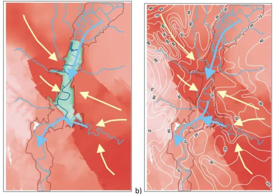
Fig 2.6: Conceptual scheme of inflows in the alluvium complex; the upper picture shows the alluvium inflows in the area of the Paleo-Tiber sedimentary graben, while the lower one shows inflows in the other areas.

14

a) b)

Figure 2.7: a) Visualization of inflows in the portion of Tiber River valley excavated inside the Paleo-Tiber Graben.

White arrows indicate the groundwater flux from volcanic and pre-volcanic aquifers toward the Aniene and Tiber alluvial valleys. The blue arrows indicate the flux direction of groundwater within the recent alluvium complex B)The isolines of the top of water table (from Capelli et alii 2008) confirm the main direction of groundwater.

In the Tiber valley alluvial complex, the wide range of hydraulic conductivity values, related to different depositional facies (see geothecnical characterization on chapter 2.3.4), influences the groundwater circulation; technical reports for “Metro C” subway line works (Lanzini M., 1995-2000 a and b) describe that groundwater flow is absent in areas with high percent of pelitic fraction and organic matter, as between Largo Torre Argentina and Piazza Venezia,; where the sandy and silty-sand fraction increases, as in the area between Piazza Argentina e Viale Mazzini, an aquifer can be recognized, hosted by the sandy and coarse-sandy facies, and having variable transmissivity and hydraulic gradient. As a general scheme, it can be observed that the sandy and coarse sandy lens and levels constitutes unconfined or semi-confined aquifers depending on the presence of confining clayey levels (which act as aquiclude) (see fig. 2.11). The hydraulic gradient measured inside the sands lens in the hystorical center of the City is very low (i=0.002) (Lanzini M., 1995-2000 a and b).

The alluvial basal sandy-gravels host a confined aquifer which head is often higher than the Tiber River stage and, thus, higher than the sandy alluvial aquifer’s stage.

15

Fig 2.8: location of areas of Piazza Mazzini, Largo di Torre Argentina, Piazza Venezia and Ponte Marconi

Head measurement in the hystorical center (technical reports, works for “C” subway line, Metro C” Geostudi, 2007-2009), show, with some exceptions, equal or higher head level for gravel aquifer respect to the sand. Southernmost, in the Valco San Paolo area, the gravels mean head is 50 cm higher than the sand head, as measured by the Roma Tre LinQ (Laboratorio di Idrogeologia

16 Numerica e Quantitativa, Università Roma Tre) piezometers and hydrometric station Tiber -“ Ponte Marconi” since september 2009 (fig. 2.9).

By those data, it can be assessed that the aquifers hosted by the sand lens and in the gravel bed can have different hydraulic relationships, that are function of the stratigraphy; where several meters of clay separate sands and gravels the two aquifers show different head, while where sands and gravels are not isolated each other by clay, a similar head can be observed in both aquifers.

The alluvial aquifer is strongly connected to the river, as observed in monitoring wells and hydrometers at “ Ponte Marconi” –Valco San Paolo (fig. 2.9).

Figure 2.9: field measurements in the Valco San Paolo area (Roma Tre LinQ gauging station at Ponte Marconi and piezometers); the sands head is lower that the gravels head; also, the strong connection between the Tiber River and the aquifer can be observed.

2.2.2

Hydrogeological complexes

Here is a description of the main hydrogeological complexes from Capelli et alii, 2008; authors recognized complexes starting from the geological complexes by Funiciello & Giordano 2008 (Carg Project, 2008); terrains and rocks having homogeneous hydrogeological features were grouped together, so that a single hydrogeological complex can include facies from different geological formations; this is because of the lithological and, thus, hydrogeological heterogeneity of the geological units. Synthetically, table 2.1 shows how the complexes described above were grouped together according with their hydrogeological rule in the Rome’s groundwater system.

0 50 100 150 200 250 300 15/09/2009 0:00 25/09/2009 0:00 05/10/2009 0:00 15/10/2009 0:00 25/10/2009 0:00 04/11/2009 0:00 14/11/2009 0:00 24/11/2009 0:00 le v e l (c m ) date

17 Tab. 2.1: list of hydrogeological complexes a coded in Funiciello & Giordano, 2008 and this study

Reference code (from Funiciello &

Giordano, 2008)

Simplified

code (this study) HYDROGEOLOGICAL COMPLEX

VGU AA Valle Giulia Formation complex

AEL AA Aurelia Formation complex

a1 AR Lacustrine deposits and alluvium Holocene –clay- complex a2 AR Lacustrine deposits and alluvium Holocene –sand - complex

l AR Lacustrine deposits and alluvium Holocene –gravel- complex FTR e FTR1 AT Fosso del Torrino Formation complex

MVA MV Monte Vaticano Formation complex

MTM1, PGL4b e

PGL3b MV Sandy clay, sandy silt and sand complex

FCZ PGT Complex of gravels and calcareous and siliceus clasts of Fosso della Crescenza Formation complex

MDP e PGL2 PGT Complex of sandy clay of Monte delle Piche and Ponte Galeria formation

PGL4a, PGL1 e

PGL3a PGT Complex of gravel and sands of Ponte Galeria formation complex VTN e SKP PGT Complex of gravel and sand of Vitinia e dell'Unità di Saccopastore

formation

MTM2 e PGL3c PGT Complex of coarse sand of Monte Mario and Ponte Galeria formations

CIL PGT Fluvial- palustrinei S. Cecilia complex

h RP Holoceneantropic landfill complex

h1c RP Quarry waste deposit complex

TDC, PTI e KKA VTA Alban Hills “Pisolitic Tuffs” complex VSN2 e VSN3 VTA Alban Hills “Pozzolanelle” complex SLV e VSN1 VTA Alban Hills “Lionato” Tuff complex

RED e PNR VTA Alban Hills “Red and black Pozzolane” complex TIB, PPT, SKF, RNR,

LLT e NMT VTA Sabatini volcanic complex

LLL, FKBb e FKBa VTAl Alban Hills Lava complex

MAK, MNN e TAL VTC Complex of Alban Hills “Peperino di Albano”, “ Valle Marciana” units and “ Tavolato” formation

In the following complexes description, the first code, written in italic, is referred to the classification used in this study, while the second one represents the code from by Funiciello & Giordano 2008.

A) Complex of Monte Vaticano Formation (MV - MVA). Gray clay and blue stratified clay. Since this complex reaches very high thickness and very low permeability values, it works as an aquiclude for the entire aquifer system. Recent boreholes drilled in this complex shown that there’s a not negligible fraction of silty sand (LinQ, 2010).

B) Complex of the alternance of sandy clay, sandy silt and sands (PGT - MTM1 and PGL3b).This complex includes the sandy-clayey facies of Monte Mario Formation (“Farneto” member,

18 MTM1) and Ponte Galeria Formation (“Monte Ciocci” and “Pisana” members). Since the hydraulic conductivity of this complex is very low, represents the aquiclude of the groundwater system.

C) Complex of coarse sands (PGT - MTMb & PGTb). Includes the coarse sand terms of Monte Mario and Ponte Galeria Formations. The complex has a very heterogeneous permeability, which can globally be considered medium high.

D) Complex of gravels and sands (PGT - PGTc). Includes gravels from Ponte Galeria Formation. This complex has a very high hydraulic conductivity and hosts an high-potential aquifer. In the hydrogeological model, this complex is included in the complex “C”

E) Complex of gravels of Crescenza Formation (PGT - FCZ). Mostly made by Fluvial gravel in a sandy matrix, sands and clays; clay layers become more frequent in the uppermost portion of the sedimentary sequence, that means from -10 m a.s.l. upward. The complex, belongs to the “Paleotiber2” lithofacies; drilling shown that the thickness of this complex is higher than 100 meters. This deposit has got a very high permeability, and can host confined aquifers. In the hydrogeological model, this complex is included in the complex “C”.

F) Fluvial-palustrine complex “Santa Cecilia” (PGT - CIL). The complex is made by heterogeneous lithotypes (from gravel to silt), with volcanic material; it has a low permeability. It is able to exchange water with the volcanic plateau and the recent fluvial alluvium. In the hydrogeological model, this complex is included in the complex “C”

G) Complexes belonging to the Alban Hills Volcanic district (VTA). Here is an overview of the main complexes belonging to the Alban Hills Volcanic district. In the hydrogeological model, the Alban Hills Volcanic formations constitute one single complex.

• Pisolitic Tuffs (PTI): pyroclastic flow deposit with very low permeability, also due to the high number of paleosolis.

• Red and Black Pozzolane (RED, PNR): pyroclastic flow deposit with massive and chaotic fabric; the permeability is medium-high and it is both for porosity and fracturation. The high transimissivity and continuity of this deposits makes it one of the most important aquifer in Rome.

• Lionato Tuff (VSN1): pyroclastic flow, with massive and chaotic fabric, very lithoid for effect of zeolithyzation, which is responsible also of the medium-low hydraulic conductivity; it works as an aquitard, isolating the surface circulation from the deeper one.

• Villa Senni Tuff (VSN2): massive and chaotic deposit, sometime with high consistence. Generally this pyroclastic unit has got a coarse matrix. The medium high permeability values, the large thickness and areal extension makes it able to host a medium transmissive aquifer.

• Lavas: this facies is referred to Vallerano Lavas (LLL), Capo di Bove Formation Lavas (FKB); the permeability is high due to the fracturaction.

19 H) Sabatini Mt. Volcanic Complex (VTA - TIB, PPT, SKF, RNR, LLT, NMT)

This complex groups mostly pyroclastic flows, and undifferentiated fall deposits, outcropping either in the right and in the left bank of Tiber River, and they are referred to the following units (from Mattias & Ventriglia, 1970): “Red tuff with black scoria”, “La Storta stratified tuffs”, “Sacrofano Varicolori stratified tuffs”. The granulometry is the one of a fine sand, with abundance of silty matrix. The whole permeability of the complex ranges from medium to medium –low, but it can be affected by local variations of the hydraulic coefficient due to the presence of several argillified paleosoils.

I) Holocene alluvium (AR)

The complex includes the alluvium of the main rivers and streams and the alluvium still in evolution inside the embankment of Aniene and Tiber rivers.

Due to the fluvial depositional mechanisms, the alluvium is made by a wide range of depositional facies; coarse sediments are related to high energy-channel areas, while silty and clayey sediments are related to areas of low energy such as alluvial plain or fluvial-palustrine environment.

The general setting of the sedimentary alluvium valley is sketched in figg 2.10 and 2.11.

F.a The uppermost unit is the A, the “historical” alluvium unit, silty clay covering homogeneously all the area. This unit has an high consistence testifying a subaereal exposition and relative oxidation of the uppermost brown colored level, and several water level fluctuations.

F.b1: Below the A unit, there are silty sand and fine sands belonging to B1 unit

F.b2: The coarse sand of unit B2 covers the unit C in the Tiber right bank, while in other parts unit B2 and unit C are in etheropy. On the left bank, unit B2 covers directly unit D1.

F.c: the unit C is gray clay with peat; the deposition of this unit occurs contemporary to the unit D1 in the Tiber right bank, while in the left bank unit C is mostly missing. During the deposition of unit C, also starts the deposition of the alluvium of Cremera- Valchetta stram(Castel Giubileo - north city ring road area) with deposition of coarse-sandy sediments fining-upward until fine sands. Those sediments are partially interfingeredto main river alluvium.

F.d: immediately above the basal gravel bed, there are coarse sands (D2 unit), sedimented in a medium energy- braided plain environment and sandy silts (D1 unit), sedimented in low energy environment.

20 F.g: discontinuous bed of basal gravel which thickness ranges between 0 and 10 meters. This deposit represents the first-high energy fluvial environment during the first phase of sea level rising at the end of the Wurmian glacial period.

J) Landfill (RP): This complex includes heterogeneous anthropic deposits. It can constitute a relevant aquifer complex when it occurs with large thickness, since its permeability is medium, and it can give local diversion of the main drainage. In the hydrogeological model, this complex is included in the complex uppermost Layer 1, representing volcanic formations.

Fig 2.10: stratigraphic relationship scheme of the Tiber alluvium; R= landfill; PL= plio-pleistocene complex.

Geologic and hydrogeologic data from LINQ and Igag-CNR were integrated in a database, which structure has been built for geologic modeling. The data archiving permits to easily extract geological features (as complexes top and bottom elevation) and hydrogeological parameters measurements.

21 Fig 2.11: Cross section of the Tiber River alluvial valley, drawn trough the Historical center (from Igag-CNR

Urbisit informal meeting, 2008)

2.2.3

Hydrogeological database

The UrbiSit-LINQ database was built to collect geological, geothecnical and hydrogeological data. The hydrogeological section has been created to collect wells and springs data. The main inputs for the roman area are data from Ventriglia (1971 and 2002), public agencies (ISPRA-Istituto Superiore per la Protezione e la Ricerca Ambientale) and private companies reports (as works for “B1”, “C” and “D” subway lines, parkings, railway roads, etc.). Those elements are inserted as record in the main table “DATO PUNTUALE “, in which all the spatial information and identity characteristics of every object can be specified:

-identifying code(which is the primary key for the entire database) -source of the information (idfonte)

22 -old code owned by the object (idoldato)

-coordinates

-topographic elevation above the sea level as reported in the original data. -topographic elevation of data extracted by the Digital Terrain Model. -place (City, municipality) and address;

- notes

The “DATO PUNTUALE” table is connected to the two tables “perforazione” and “sorgente”, in which are specified characteristics of the two main types of hydrogeological data that can be inserted: wells and springs.

In the table “PERFORAZIONE” characteristics of wells are carried:

-use of the well (which is: for irrigation, drinkable wate, piezometer, etc.)

-type of the piezometer (“tubo aperto” o “Casagrande”), in case the use of the well is as piezometer; -dynamic discharge of the well (liter/sec);

-Transmissivity and storage coefficient which are calculated from pumping tests; -presence of gas in the water of the well;

The table “FALDA” Is connected to the table “PERFORAZIONE” by a relationship “one-to-many”; in this table there are informations about aquifers which were encountered during the drilling; here there can be specified:

- depth of aquifer top and bottom respect to the surface;

- depth of aquifer top and bottom above the sea level as reported in the original data; - depth of aquifer top and bottom above the sea levelas in the Digital terrain model; -notes related to encountered aquifers.

The table “FILTRO ” is connected to the table “PERFORAZIONE” by a relationship “one-to-many”; in this table there are informations about the well screen:

- depth of screen top and bottom respect to the surface;

- depth of screen top and bottom above the sea level as reported in the original data; - depth of screen top and bottom above the sea levels as in the Digital terrain model; -notes related to screen.

23 The table “PERFORAZIONE” is connected to the table “MISURA PARAMIDRO”, in which there are informations about static and dynamic head measurements and the chemical and physical characteristics of water. The connection is by a relationship “one-to-many”, so that it is possible to insert more than one measure for the same well; issues in this table are:

-static and dynamic head respect to the surface;

-static and dynamic head above the sea level as reported in the original data; -static and dynamic head above the sea level as in the Digital terrain model; -well dynamic discharge, from which hydrogeological parameters can be known

- chemical and physical characteristics of water in the well, as: temperature, electric conductivity, presence of gas.

The table “PERFORAZIONE” is connected to the table “STRATIGRAFIAPERF”, in which are inserted informations about top and bottom elevation of each drilled layer, plus the related description. The table “STRATIGRAFIAPERF” is related by the primary key “ididro” to the table “IDROGEOLOGIA” by a relationship “one-to-one”; in this table, data about hydraulic conductivity can be inserted for the considered layer. This is what can be inserted:

- Hydraulic conductivity (k) in m/s;

- Type of (k) measurement; k can be measured in the field by slug and pumping tests or in laboratory (i.e. edometric prove);

- Derived Hydraulic conductivity, which is k deducted by literature, or from geotechnical data or from granulometric curves.

The table “IDROGEOLOGIA” is connected to the table “INTERPIDROGEOLOGIA”, in which k values can be associated to a hydrogeological code. This table makes easier the geological interpretation because layers with very similar k values can be assimilated in the database, with the same hydrostratigraphic code; indeed, the relationship connecting “IDROGEOLOGIA” and “INTERPIDROGEOLOGIA” is a “many to one” relationship. Fields in this table are:

- “Idintstratidro”, where can be inserted the code assigned to the hydrogeological layer, which are the codes listed in table 2.1, chapter 2.2.2, “Hydrogeological complexes”

- “Descrizione”, where is reported the description of the hydrogeological layer;

- the field “IDROSTRAT IGRAF” contains the code used for the stratigraphic interpretation;

-For each recognized hydrostratigraphic unit is reported the corresponding cartographic code, referred to the geological map of Rome in scale 1:50.000 (Funiciello & Giordano, 2008).

-it is reported also the code corresponding to the UrbiSit 2008 project, which can be considered a simplyfied version of the cartography.

24 -finally, the table contains a qualitative k classification for each hydrostratigraphic unit.

The scheme of the relationships between the database tables is in attached n1

2.2.4

Building main hydrogeological surfaces

The geological modeling process in this study is aimed to reconstruct the hydrogeological properties of geological complexes featuring the subsoil of the central and northern part of Rome, around the path of the Tiber River. The study is focused on the geological framework around the valley and the hydrogeological relationships between the Plio-Pleistocene substratum and the alluvial deposits. Besides the top of the basal gravel alluvial deposits has been reconstructed, that can be considered as a semi-confined aquifer, to understand its hydrogeological potential. Geological formations of which we reconstructed surfaces were engraved during Holocene by the erosion of Tiber and minor rivers flowing

into Tiber, and this produced the need to

reconstruct also the morphology of the alluvial valley, meaning the morphology

containing the recent alluvium. This was possible thanks to drilling data

depth of alluvium and according to extrapolations reasonings on fluvial dynamics mechanisms. The reconstruction involved, in addition to the Tiber and Aniene rivers valleys, confluence zones of Crescenza stream and Valchetta stream in Tiber valley, because they have an high thickness of permeable deposits in contact with Tiber basal gravel and so they can give an important contribution to the hydric recharge of these deposits. The modeling process includes both well data and GIS analysis. At first we managed the large number of well data to derive the backbone of the geological model by coding operations. Then, using Arcgis® tools we integrated the main surface information given by the Geological map 1:50.000 of Rome municipality (Funiciello R., Giordano G., 2008) and also local data derived by cross sections obtaining a complete data set of the main boundary surfaces as recognized in the reference stratigraphic frame.

managing well data

In the study area there are 2950 point data belonging to the Urbisit database, among which 938 drillings and 1219 point of measurement of groundwater level were selected.

To better constrain the coding operation for the geological modeling, a quality ranking was established, basing on the following criteria:

- Well Depth;

- Ratio well depth/number of geological levels described in the well log ;

- Nearness to a stratigraphic limit in the geological map 1:50.000 of Rome municipality (Funiciello R., Giordano G., 2008)

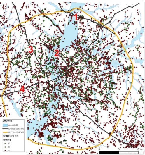
25 According to this criteria, a score was assigned to each well and three ranking classes where distinguished (A,B,C); wells which are considered more reliable for geological reconstruction belong to the highest score class (fig 2.12).

Figure 2.12: distribution of boreholes in the whole urban area of Rome.

All boreholes belonging to the class (A) in the study area (326 drillings) where analyzed and coded according to the stratigraphic reference frame of tab.2.1. Boreholes with highest ranking class (A) were used to draw two geological cross sections by means of stratigraphic correlations between similar multilayer. The geological framework as reconstructed in cross sections was used to analyze and codify also medium and low quality wells (B and C classes) which are placed close to their traces of cross sections. Cross sections are in fig 2.4 and in attached n2.

A multiple step procedure has been followed to build the main geological surfaces taking into account all the available data; the flux diagram of tools that have been used is in figure 2.13.

A) Each well data having the same code (for instance PGT) and therefore belonging to the same geological unit was extracted from the database. In the case of more than one level

26 of the same unit in a single well, the one with the highest elevation that was identified as the top surface was pinpoint;

B) By using an Arcgis® tool developed by Igag-Cnr, cross sections (see fig. 2.4 and attached n. 2)were digitized; moreover, for building surfaces were used also cross sections drawn in the Urbisit project 2008. For every top surface drawn on each section, points were extracted with z value, and added to the datasets extracted from the well data;

C) In order to include in the geological reconstruction the limits of each main surface as drawn in the vector geological map, the feature to pointArcgis® tool in data management toolbox was used to obtain a point dataset featuring the limits. Therefore, the extract values to point Arcgis® tool in spatial analyst/extraction was used in order to assign the corresponding Digital Model Terrain (with resolution 20 x 20 meters) elevation value; D) To better shape the geological surface, not only the limits of outcropping polygons were

considered, but a network of points was added within each polygon of the geology shape file; point network was derived by a sequence of GIS operations. The geology polygons were converted in raster format trough the polygon to raster Arcgis® tool in the conversion toolbox and then each raster was converted in a point shape file by the raster to point tool in the conversion toolbox. Finally, by using the tool extract values to point in the spatial analyst toolbox, elevation values from the DTM were extracted and added to each point. The point network was added to the points dataset obtained by well data and cross sections.

E) The definitive points dataset was interpolated using the IDW (inverse distance weighted)algorithm in the Arcgis ® Geostatisical Wizard tool; fault shape files has been used as barrier polyline.

27

Figure 2.13: Flux diagram showing Gis tools used to build hydrogeological surfaces.

Top surfaces of the geological units featuring the subsoil of the central-northern part of the city of Rome surrounding the Tiber River were reconstructed; then, the maximum erosion surface of the Tiber River and main tributary streams were also built, and the top surface of the basal gravel level inside the alluvial filling.

28 The bedrock of the Tiber alluvial deposit is featured by three main geological complexes: the late Pliocene-early Pleistocene marine clayey and sandy-clayey of the Monte Vaticano-Monte Mario units; the lower-middle Pleistocene “Ponte Galeria” unit; the middle-late Pleistocene volcanic complex, including coeval sedimentary deposits.

The Monte Vaticano-Monte Mario (MV-MM) units as a whole, has been considered as an aquiclude. In the western part of the study area, along the right bank of Tiber River, the top surface of such hydrogeological complex (Figure 2.14a and 2.14b) reaches the highest elevations, outcropping at 130 m a.s.l. in the Monte Mario structural high. This last is bordered on the Eastern side by N-S and NW-SE trending normal faults dipping towards the East and North-East that rise the Plio-Pleistocene sedimentary complexes on their footwall.

The central and eastern zones of the study area are characterized by lower elevations; the MV-MM top surface is downthrown by main tectonic lineaments and lowered up to 90 m b.s.l. at the base of a NW-SE oriented tectonic depression known as to Paleo-Tiber Graben (Funiciello et alii, 2008 and reference therein). Between the Monte Mario structural high and the Paleo-Tiber graben, the MV-MM top surface evidences erosional features as secondary streams flowing into the main graben and isolated morphological reliefs, as for example beneath the actual position of Termini station (40 m a.s.l.).

Above the MV-MM top surface, we distinguished the boundary erosive surface between the Ponte Galeria sedimentary unit and the overlying volcanic multilayer (PGT top formation, Figg 2.15a and 2.15b). The absolute elevations show a decreasing trend of the PGT top surface from the North-Western sector along the right bank of Tiber River, ( 100 m a.s.l.), towards South-East, (up to -40 m a.s.l.).

There’s a nearly-complete filling of the Paleo-Tiber Graben: from drillings and literature (Florindo et alii, 2007) is indeed well-known that in the graben area the thickness of fluvial-deltaic sediments deposed since lower Pleistocene onwards exceeds 100 meters.The lowest elevation in the south-east sector can be related to the NE-SW trending fault linked to the volcano-tectonic activity of Alban Hills.

The surface of maximum erosion of the fluvial deposits (figures 2.16a and 2.16b) shows the local morphology precedent to the last depositional cycle, which occurred since the Holocene, of the alluvial complexes of Tiber River and his main tributary: the Aniene river, Crescenza e Valchetta streams.

The main valley (Tiber River Valley) has a quite regular flat floor with variable width ranging from 200 meters to 2 Km; the alluvial valley narrows at the Villaggio Olimpico zone, between Ponte Flaminio and Villa Glori, and widens at the confluence with Aniene tributary. The lowest elevation at the center of the valley is about 52 m b.s.l..

29 a)

b) Figure 2.14: a)reconstruction of the bottom of Ponte Galeria Formation (equivalent to the top of Plio-Pleistocene). b)Contour map resulting from the grid interpolated with kriging method and corresponding surface. The coordinate grid is referred to ED50 N33 projected system.

30 a)

b)

Figure 2.15: a)reconstruction of the bottom of volcanic formations (equivalent to the top of Ponte Galeria Formation). b)Contour map resulting from the grid interpolated with Inverse distance weighted algorithm and corresponding surface. The coordinate grid is referred to ED50 N33 projected system.

31 a)

b) Figura 2.16: a)reconstruction of maximum erosion of alluvial Tiber Valley b)Contour map resulting from the grid interpolated with IDW method and corresponding surface. The coordinate grid is referred to ED50 N33 projected system.

32 Fig 2.17: Geological model buit in this study: the exaggeration is to better show the stratigraphic relationships. The black surface is the DTM; the green surface is the bottom of volcanic complexes and the blue surface is the bottom of the Ponte Galeria Formation.

The top surface of alluvial basal gravels was built by selecting 107 boreholes, drilled for the whole length of the alluvial valley. This complex includes the basal gravel beds of Tiber and Aniene rivers and the gravel, sandy gravel and coarse sands of minor tributary Crescenza and Valchetta streams. Tributary streams alluvium have been assimilated to the oldest Tiber basal gravel bed in the first level reconstruction, because they’re made by sediments very similar in hydraulic conductivity and,

33 moreover, they’re in stratigraphic contact; tributary alluvium give an important groundwater recharge to the Tiber alluvium.

The top of basal gravel has been built only in area with a reasonable amount of stratigraphic data, which is from the Northern part of the city ring road till the south border of the study area.

The distribution of stratigraphic data is discontinuous; in the areas of Fidene station, Urbe airport and Tor di Quinto hippodrome there are no data, while in the area from Olympic Stadium to Testaccio Hill there’s a great number of data.

The Isobaths of top of basal gravel were built manually; then, with the TOPO TO RASTER Arcgis® tool, the corresponding interpolated raster was built.

The top of basal gravel surface ranges from 0 to -68 m a.s.l.; this surface’s general trend shows absolute top heights decreasing from the borders of the valley (where the top of gravels is on average at around -20 m a.s.l. towards the center (where the top reaches heights till -47 m a.s.l.)

In general, top heights at the center of the valley show a general decrease from the Northern zone (Castel Giubileo) where they are found at -30 m a.s.l. towards South (Tiberina Island-Testaccio), where top heights are the highest of study area (-47 m a.s.l.).

In tributaries confluence areas, the top of this surface is considered high because of the thickness of tributary’s sediments.

The thickness of the “basal gravel” complex ranges from 0 to 40 meters. The thinnest parts are those close to the border of the valley; the thickest are in the confluence areas.

In particular can be noticed the elevated thickness in the confluence zone of Valchetta stream, where sediments with high permeability are found from the height of 0 m a.s.l..

In the area Monte Mario - Olympic Stadium there’s a zone where the top of basal gravel ranges from 12 to 16 meters b.s.l., higher than the immediately eastern area, where the top is at around 30 meters b.s.l.. The origin of this discrepancy could be due to tectonic, as a fault segment trending NE-SW.

34 Fig. 2.18: reconstruction of the top surface of the silty-gravel bed in the Tiber alluvium.

35

2.3

Hydraulic properties

Hydraulic conductivity (k) values come from field measurements and from geotechnical laboratory tests (see chapter 2.3). Field data include slug tests (Lefranc permeability tests) and pumping tests, distributed in the study area as shown in fig. 2.19. Proves have been performed over all the types of alluvial terrains. Regarding the volcanic complexes, in the study area (considering a 3 km buffer around the boundary) there are 17 tests. Due to the high k heterogeneity of volcanic rocks, those tests are retained insufficient to represent volcanic hydraulic conductivity for the whole study area. Four pumping tests concern the sedimentary PGT complex, located along the path of Crescenza stream.

36 Due to the small number of test and to the wide range of measured k values for each complex, values assigned to complexes also derive from literature data and from regional numerical models developed by the LINQ; in some case, the knowledge about granulometry and possible transmissivity has been sued to derive an initial value.

2.3.1

Volcanic complexes

Two volcanic complexes are present in the study are: the Sabatini Volcanic complex and the Alban Hills volcanic complex. The Sabatini Volcanic complex includes mostly stratified tuffs, and, according to regional hydrogeological models developed in the Laboratory of Hydrogeology of Roma Tre University (LINQ) in the Sabatini Mts. area, one single hydraulic conductivity value of was assigned to the whole complex. The value for kx-ky (2.13 m/d) is the calibrated value for regional model (see tab 2.2), while the kz value was kept fixed in the Sabatini model as 1E-6 m/s, which is 0.0864 m/d.

For the Alban Hills volcanic complexes, in the study area are present “Red and Black pozzolana” and the “Villa Senni” Formation (Funiciello & Giordano, 2008), with the two lithofacies “Villa Senni tuff” and “Lionato Tuff”; Villa Senni formation hydraulic conductivity is lower than units “Red Pozzolane” and “Black Pozzolane” due to the zeolithization and presence of cineritic interbeds. As in Sabatini complexes, in the Alban Hills volcanic products the presence of argillified paleosoils is the reason for the reduced vertical hydraulic conductivity (kz) respect to the horizontal one (kx, ky).

Tab 2.2: average values for volcanic complexes (LINQ, 2010)

2.3.2

PGT Formation complex

The sedimentary prevolcanic complex (which we refer to as PGT Formation complex) is mostly present as the Fosso Crescenza-FCZ facies; in order to assign a transmissivity value to the FCZ formation, it was considered as a homogeneous multilayer sequence of gravel-sand and clay, where gravel and sandy terms are more transmissive while clay layers are mostly aquitards; because of the low number of deep boreholes drilled in the FCZ formation, a reconstruction of different facies inside the FCZ is not possible; in fact, the extreme spatial variability of the sedimentary formation and the lack of deep well makes hard to distinguish the different facies which are in contact with sediments in the valley. The multilayer conformation derives from data

unit K x(m/d) K z(m/d) notes

Sabatini stratified tuffs 2.13 0.0864 Sabatini complex volcanic units “Villa Senni” Formation 0.1728 0.015552 Alban Hills volcanic complex Red and Black Pozzolane 6.048 2.592 Alban Hills volcanic complex

37 on deep boreholes in the Bufalotta-Talenti area. These 90 meters-deep continuous coring boreholes show a stratigraphy for FCZ sequence made by three sandy-gravel layers separated by three clay aquitards (fig 2.20).It can be assumed this stratigraphy as continuous for all the FCZ deposit inside the graben, and from this assumption an average transmissivity can be calculated.

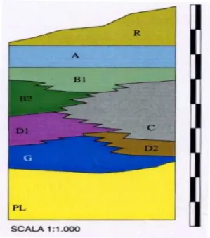
Figure 2.20: sketch of the multilayer FCZ Formation (from drillings in Bufalotta-Talenti area, LINQ 2010). Height scale: 1:500.LENGHT SCALE: 1:1000. 1) Volcanic complex; 2) PGT, silty-sand facies; 3) PGT, sand facies; 4) PGT, clay facies; 5) PGT, sandy-gravel facies; 6)Plio-Pleistocene overconsolidated clay.

The average transmissivity for each layer is computed by multiplying the average k values (from literature data) times the thickness; the total transmissivity of the multilayer as a whole is calculated by adding together the transmissivity of every single layer.

The clay part is silty clay with thin peat layers; the average k value that can be reasonably assigned is 0.000397 m/d according with the slug tests in the clay layers close to the Crescenza Stream. The average thickness is about 26 meters. The sandy-gravel unit is made by clasts having centimetric and decimetric diameter in a sandy-clayey matrix, not consolidated; the average k value that can be reasonably assigned is 0.292 m/d according with the slug tests in the sand-gravel layers close to the Crescenza Stream; the thickness is 30 meters. The computed transmissivity for the whole FCZ deposit is then calculated as 8.77 m2/d. The average hydraulic conductivity that can be deducted is 0.14 m/d for horizontal hydraulic conductivity, and 0.014 for vertical hydraulic conductivity.

38

2.3.3

Plio-Pleistocene units

Since the “bedrock” aquiclude formation (Marne di Monte Vaticano, MAV) is not hydrogeologically productive, there are no slug or pumping tests. Initial hydraulic conductivity was chosen in order to give a very low permeability to layers 3-8 external to the Tiber Valley. The initial assigned k value was Kx=Ky=0.1m /d, kz=0.01.

2.3.4

Alluvium complexes

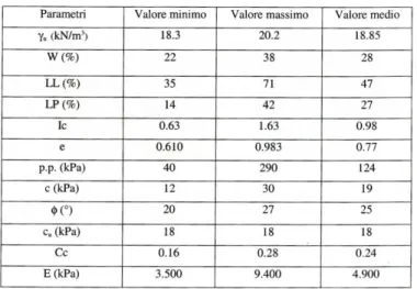
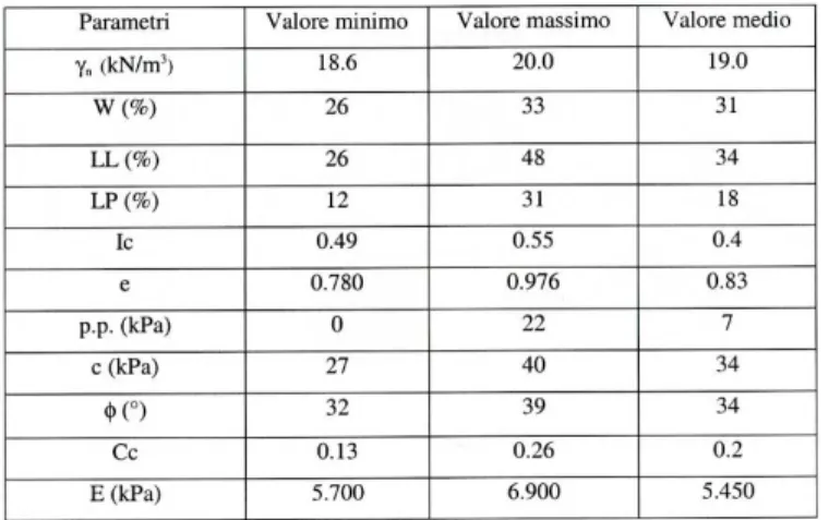
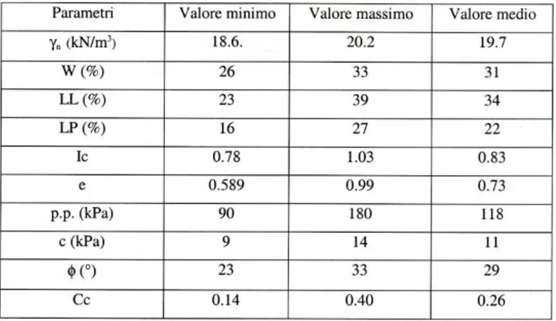
Alluvium complex is featured by a huge heterogeneity; authors recognized many lithofacies composing the complex, which are listed in table 2.3. The following tables and histograms briefly show the main geotechnical characteristics of Holocene Tiber River alluvium (data from laboratory geotechnical proves made by LINQ in 2002 and from geothecnical reports for “C” subway line works by Lanzini M., 1995-2000a and Geostudi, 2007-2009).

Tab 2.3: classification of Tber alluvium as recognized by from laboratory geotechnical proves made by LINQ in 2002 (LINQ, 2003)

Alluvium unit A1 - hystorical silty clay

A2 - hystorical silty clay with green sands B1 - sand and silt

B2 - coarse sand (upper) C - clay with peat D1 - silty sand

D2 - coarse sand (lower) G -basal gravel

39 Fig 2.21: measured parameters for geotechnical group A1

Fig 2.22: measured parameters for geotechnical group A2

40 Fig 2.24: measured parameters for geotechnical group B1

Fig 2.25: histogram of granulometric fraction for group B1. The large fraction of sand and silt can be observed.

41 Fig 2.27: histogram of granulometry for group B1. The sand fraction is prevalent; a small amount of gravel can be noticed.

Fig 2.28: measured parameters for geotechnical group C

42 Fig 2.30: measured parameters for geotechnical group D1

Fig 2.31: histogram of granulometry for group D1. All the granulometric fraction, except the gravel one, are represented.

We don’t have geotechnical characterization for group D2, since it’s made by gray coarse sands. For the “basal” sandy gravel is reported the granulometric fraction histogram (technical reports, “Metro C” subway line, Lanzini M., 1995-2000a )

43 Fig 2.32: granulometric fraction histogram for group G. The sand fraction is prevalent; the fraction of gravel is around 39% (Lanzini M., 1995-2000 a and b, modified).

The histogram Fig 2.32 refers to gravel samples coming from the hystorical center; due to its wide textural heterogeneity, the sandy-gravel complex shows different percentage of matrix and different matrix granulometry (from silty to sandy) depending on the sample-sites. (fig 2.33).

Fig 2.33: Pictures of cores drilled in three different sites along the path of “C” subway line (“Metro C”) In this study’s hydrogeological modeling, alluvium units were simplified and a total number of 5 units are distinguished (Table 2.4): the same “coded” unit can have different percentage of clay and sand, and this brings a wide range of possible hydraulic conductivities to be assigned.

0 10 20 30 40 50 60

granulometry G

44 Moreover, many authors observed an increasing of k values measured in pumping tests with the increasing of discharge (Shulze-Makuch & Chekauer, 1995), and they also observed that the increase occurs in different rates depending on the heterogeneity degree of the formation. In this study, K values for each alluvial facies come from slug tests, pumping tests, edhometric laboratory tests, and indirectly derived from granulometric curves; data come from public works in the city of Rome or in areas close to the city, as “Metro C” and “Metro B1” subway works, the Castel Sant’ Angelo underpass, San Pietro railway station, Nazzano Dam, Foro Italico-Trionfale street axis. We also considered published and unpublished literature as Bozzano (2000) or master degree’s thesis which analyze Tiber alluvium (LINQ 2003 and 2009). Figure 2.34 shows permeability tests distribution in two sample areas, both located in the Tiber alluvial valley. In Table 2.4 k for each unit are listed; both ranges and average k are taken from literature and pumping tests.

45 Tab 2.4: the table lists the 5 alluvium units considered in this study and corresponding k value range (From Bozzano 2008, LINQ 2003 and Lanzini M., 1995-2000 a and b)

Alluvium unit

Corresponding unit (Bozzano 2008, LINQ 2003,

Lanzini, 1995-2000 a and b) Min k (m/d) Max k (m/d)

Average k (m/d)

Landfill RP 0.1

0.01 0.055

Clay and silty clay A, 0.00003456

2.59 1.03421376

Sand B1, B2, D1, D2 0.03222 43.2

8.8527312

Clay with peat C 0.00001728 0.01728

0.5214312

Gravel G 0.003

6.5 1

One of the purpose of Roma model is to find a k value which reproduces the effective hydraulic conductivity of the hydrogeological unit at a regional scale, despite of small scale heterogeneities that can locally change the measured hydraulic conductivity. In table 2.5 the k values chosen as initial k values for the model are resumed; in some case values are far differ from data listed in Tab 2.4.K values will be subjected to calibration in the numerical model phase.

Tab 2.5: Initial k values assigned to complexes

K zone lithotype Kx, Ky (m/d) Kz

1 Volcanic complex- Alban Hills 6.04 2.5

2 Volcanic complex- Sabatini HIlls 2.13 0.0864

3 PGT complex (Paleo-Tiber) 0.14 0.014

5 Alluvium- clay and silty clay (A) 0.1 0.01

6 Alluvium- sand (B1,B2,D1,D2) 2 0.2

7 Alluvium- clay with peat (C) 0.1 0.01

8 Alluvium- gravel (G) 4.2 0.42

8 Alluvium- clay, also bedrock 0.01 0.001

46

2.4

Aquifer system inflows and ouflows

2.4.1

Climate feature

Precipitations in the study area occurs with an average of 650 mm/y (Fig 2.35) and are concentrated in a restricted time comprised between autumn and spring, often occuring in intervals of more consecutive days. Data come from the SIMN- Istituto Idrografico e Mareografico Nazionale.

Fig 2.35: statistic interpolation of rainfall data ( 1997-2001) and location of SIMN measurement sites. The average rainfall in the study area ( for the period 1997-2001) is 650 mm/year. (from Capelli et alii, 2005) Temperature and rainfall data recorded by SIMN stations used for the study of volcanic aquifers show, during the period between 1980 and 2000, an increasing trend in the average annual temperature and a decrease of annual precipitation (150-200 mm in 20 years) (Capelli et al.,

47 2005), that, consequentially produces a decrease of effective infiltration. See Tab. 2.6 for the process that has been followed to elaborate climate data.

The recharge has been calculated by the distribute balance method as reported in Capelli et alii, 2005; the annual recharge is calculated in each cell as the difference between precipitation, runoff and real evapotranspiration. The effective infiltration is the portion of rain that contributes to aquifer recharge considered. In the case of aquifers where contributions of surface water and groundwater from adjacent areas can be considered negligible, the effective infiltration corresponds to the amount of renewable resource, and thus available for the maintenance of underground and surface outflow/inflow basis of the waterways and the many uses associated with human activities.

In different areas of the hydrological basin, the recharge takes different values depending on: - The spatial and temporal distribution of weather-climatic factors (temperature, rainfall, solar radiation, wind speed, humidity);

- The area's topography (slope, exposure, presence of drains areas and / or semi-Endor); - The nature of the aquifer lithology (rock’s permeability);

- The characteristics of soils (AWC, effective porosity etc.); - Plant cover;

- Land use.

The maximum size of computational cells must be comparable with the minimum size considered cartographic element (land use, lithological associations, morphology, etc. AWC). The timescale should allow to take into account seasonal variability and, ultimately, distribution and intensity of meteorological events. The experimental data currently available would make it the approach to scale monthly and in some cases, daily scale. Note that it is always advisable to obtain the recharge by the sum of contributions monthly or daily. This makes possible to take account of variability in several years of regional factors (variables of site) and climate (weather and climate variables). In table 2.6 is represented a scheme of the process of calculation of the recharge; the estimation of the main items (temperatures, rainfalls, runoff) is discussed below.

48 tab 2.6 : resume of parameters for distributed balance as computed in Capelli et alii, 2005

starting data kind of aggregation/other informations data processing unit of measurement and maximum and minimun value output time variable

Daily precipitations monthly cumulate precipitation

kriging, FAI-k mm P distribuited value of

monthly precipitation (grid)

yes

Maximum daily temperatures Tmax monthly mean of

the maximum daily temperatures

kriging FAI-k, with external drift

°C Tmax distribuited value

of the monthly mean of the maximum daily temperatures (grid)

yes

Minimum daily temperatures Tmin monthly mean of the minimum daily temperatures

kriging FAI-k, with external drift

°C Tmin distribuited value

of the monthly mean of the minimum daily temperatures (grid)

yes

Mean daily temperatures (obtained by the mean of the minimum and maximum daily temperature values)

Tmean monthly mean of the medium daily temperatures

kriging FAI-k, with external drift

°C Tmean distribuited

value of the monthly mean of the medium daily temperatures (grid)

yes

Corine land cover (shape poligon)

building a specific legend correlate to fotointerpretation areas colors ortophotos - scale

1:10.000 of the Regione Lazio flight of year 2000

fotointerpretation of colors ortophotos

topographic map 1:10.000 draw perimeters of the UTI

H=thickness of soil (m) -from geology map (1:25.000) shape poligon

P= gradient of stone (%) 120=mean unitary value of the reference AWC for the considered soils (mm/y) F=correction factor for vulcanic soils

UTI a monthly value of kc

is associated to every UTI class

from 0 to 1,1 Kc -distribuited monthly value of the crop coefficents (grid)

yes

hydraulic conductivity (geology)

topography slope (DEM) vegetal covering (UTI)

RA solar radiation, it has an unic monthly value for the entire area

EVR

(evapotraspiration)

EVR= ETR (if there isn't deficit)

if P+Ui>ETR

ETR= ETP*kc DF deficit

EVR= P+ Ui (if there is deficit)

if P+Ui<ETR

Surface Runoff Recharge

UTI (Unit of Territory Hydro exigency)

mapping units with homogeneous need of water (shape poligon)

yes

Value necessary in the estimation of the Evapotraspiration AWC= H*(1-P)*120 F Avaiable water capacity mm, from 0 to 235

distribuited value of the

AWC (grid)

no

Uim = (P- ETR+Ui)m-1; if Uim>AWC => Uim=AWC; if Uim<AWC=> Uim=Uim and DF= (Ui-ETR+P)m

SR(year) = Σ (Pmonth-EVRmonth)*Ck

R (year)= Σ (Pmonth- EVR month- SRmonth + Endo month)

assigning a percent value to each component

from 0 to 1 Ck -distribuited value of

the Kennessey coefficent (grid)

almost no

ETP= 0,0023 (Tmean+17,8) (Tmax-Tmin)0,5 RA