1
Alma Mater Studiorum - Università di Bologna
SCUOLA DI INGEGNERIA E ARCHITETTURA
D
IPARTAMENTO DII
NGEGNERIA DELL’E
NERGIAE
LETTRICA E DELL’I
NFORMAZIONE-D
EIT
ESI DIL
AUREAM
AGISTRALE INI
NGEGNERIA DELL’A
UTOMAZIONEFault Diagnosis of a Variable Speed Wind Turbine
via Support Vector Machines
CANDIDATO:
RELATORE:
Hamid Irandoost Prof. Andrea Tilli
No. 0000729919
CORRELATORE:
Christian Conficoni
A
lessandro BossoA
nnoA
ccademico: 2016/2107 Sessione III2
Abstract
In recent years, wind energy is considered as the most practical substitute energy to replace the fossil fuels. Wind turbines are massive and installed in locations, where a non-planned maintenance is very costly. Therefore, a fault-tolerant control system that is able to maintain the wind turbine connected after the occurrence of certain faults can avoid major economic losses.
To keep the wind turbine operational or at least safe, in severe cases, a reliable fault diagnosis methodology has to be exploited. It must detect, in the required time, any deviation of the system behaviour from its ordinary case, identify the location and type of the fault and reconfigure the control system to accommodate the so-called discrepancy.
To achieve the above goals, a vast number of methods have been suggested by many researchers all around the world. In this thesis, the promising classification framework of the Support Vector Machines is applied to fault detection for variable speed turbines, highlighting its features. In this regard, different fault scenarios are imposed on a benchmark model of a horizontal-axis wind turbine to check the functionality of the mentioned fault detector and the control reconfiguration module.
3
Astratto
Negli ultimi anni, l'energia eolica viene considerata la forma rinnovabile più adatta per sostituire i combustibili fossili. Le grandi dimensioni delle turbine, e il fatto che siano spesso installate in luoghi non facilmente accessibili, rendono le operazioni di manutenzione non pianificata piuttosto costose. Pertanto, un sistema di controllo fault-tolerant in grado di mantenere la turbina eolica collegata dopo il verificarsi di determinati guasti può evitare gravi perdite economiche.
Al fine di mantenere la turbina eolica operativa o almeno sicura, nei casi più gravi, deve essere sfruttata una metodologia di diagnosi dei guasti affidabile. Si deve rilevare, nel tempo richiesto, qualsiasi deviazione di comportamento del sistema dal suo caso ordinario, identificare la posizione e il tipo del guasto, e riconfigurare il sistema di controllo per gestire la cosiddetta “discrepanza” (di comportamento del sistema).
Per raggiungere gli obiettivi di cui sopra, diversi metodi sono stati proposti in letteratura.. In questo lavoro di tesi viene applicato il framework di classificazione Support Vector Machines alla diagnosi di guasti e anomalie per turbine eoliche a velocità variabile. A questo proposito, diversi scenari di errore sono imposti su un modello di riferimento di una turbina eolica ad asse orizzontale per verificare la funzionalità del rilevatore di guasti menzionato, e il modulo di riconfigurazione del controllo.
4
Table of Contents
Abstract ... 2 Astratto ... 3 Table of Contents ... 4 Introduction ... 7 References ... 10Chapter 1: Wind Turbine ... 11
1.1 Historical Development of Wind Turbines ... 12
1.2 The Nature of the Wind ... 15
1.3 Wind Turbine Components ... 18
1.3.1 Tower ... 18 1.3.2 Wind direction ... 19 1.3.3 Nacelle ... 19 1.3.4 Yaw drive ... 20 1.3.5 Yaw motor ... 20 1.3.6 Wind vane ... 20 1.3.7 Anemometer ... 21 1.3.8 Drive Train ... 21
1.3.9 Main (Low-speed) shaft ... 22
1.3.10 Gear box ... 23
1.3.11 Brake ... 24
1.3.12 Generator ... 24
1.3.13 Small (High-speed) shaft ... 25
1.3.14 Rotor ... 26
1.3.15 Hub ... 26
1.3.16 Blades ... 26
1.3.17 Controller ... 27
1.3.18 Pitch System ... 28
1.4 Wind Turbine Model ... 29
1.4.1 Wind Model ... 30
1.4.2 Blade and Pitch Model ... 30
5
1.4.2.2 Pitch System Model ... 37
1.4.3 Drive Train Model ... 37
1.4.4 Generator and Converter Model ... 39
1.4.5 Wind Turbine Control system concept ... 40
1.4.5.1 Wind Turbine Control Regions ... 41
1.4.5.2 Wind Turbine Controller ... 42
References ... 46
Chapter 2: Fault Diagnosis ... 47
2.1 Fault ... 48
2.2 Fault Diagnosis ... 49
2.3 Fault Tolerant Control ... 51
2.4 Fault Scenarios ... 54
2.4.1 Sensor Faults ... 54
2.4.2 Actuator Faults ... 55
2.4.3 System Faults ... 56
2.4.4 FDI Requirements ... 57
2.4.5 Fault Accommodation Requirements ... 59
References ... 60
Chapter 3: Support Vector Machines ... 61
3.1 Classification Analysis ... 62
3.2 Support Vector Machines ... 63
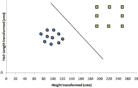
3.2.1 Binary Classification ... 64
3.2.2 Linear classifier ... 66
3.2.3 Nonlinear classifier ... 68
3.3 Optimal Hyperplane for Linearly Separable Patterns ... 70
3.3.1 Linear SVM Formulation ... 70
3.3.2 Linear SVM Formulation in the Dual Form ... 72
3.4 Optimal Hyperplane for Non-Linearly Separable Patterns ... 74
3.4.1 Soft Margin Hyper plane ... 74
3.4.2 Nonlinear SVM Classifier ... 77
3.4.2.1 Primal classifier in transformed feature space ... 80
3.4.2.2 Dual classifier in transformed feature space ... 80
6
3.5 Summary... 83
3.5.1 SVM Features ... 83
3.5.2 SVM Steps ... 84
3.5.3 Pros and Cons ... 84
References ... 85
Chapter 4: SVM Application to Wind Turbines ... 86
4.1 Applied SVM for Fault Detection in Wind Turbine ... 87
4.1.1 Phase 1 - SVM Learning ... 88
4.1.2 Phase 2 - SVM Validation ... 91
4.2 Simulation Results ... 94
4.2.1 Pitch sensor Faults ... 95
4.2.1.1 Fixed Value ... 95
4.2.1.2 Gain Factor ... 97
4.2.2 Generator and Rotor Speed Sensor Faults... 99
4.2.2.1 Fixed Value ... 99
4.2.2.2 Gain Factor ... 101
4.2.3 Converter Torque Actuator Fault ... 104
4.2.4 Pitch System Actuator Faults ... 105
4.2.4.1 Abrupt Change ... 105
4.2.4.2 Slow Change ... 106
4.2.5 Drive Train system Fault ... 106
4.3 Conclusions ... 108
References ... 109
Appendix ... 110
App.1 Quadratic optimization for finding the Optimal Hyperplane ... 110
App.1.1 Constrained Optimization by Lagrangian Relaxation ... 110
7
Introduction
Energy shortage, Due to the decrease of fossil fuel sources, and environmental pollution are two important issues of the human lives and social developments in these years. Traditional mineral energy sources such as coal, oil and gas will be used out in a few years and will cause serious environmental problems. Consequently, the renewable energy, especially wind and solar types have become very popular all over the world. Among the available options, wind energy is considered as the most practical substitute energy to replace the fossil fuel, due to its competitive cost, the maturity of technology and good infrastructure [13]. The future of wind energy passes through the installation of offshore wind farms. In such locations, maintenance costs in an unpredicted situation grow drastically. Hence, a fault-tolerant control system that keeps the wind turbine operational, even after any fault incidence, avoids huge economic impacts.
Wind turbines exhibit behaviours like wind-generated noise, nonlinear aerodynamics, vibration in the components that might potentially lead to a fault. Recently, Process Fault Diagnosis (PFD) systems have been developed to a high degree of quality in modern industry to avoid severe damages. The objective of fault detection is to generate auxiliary signals based on measurements and rules, which highlight whether the considered system is running in nominal or faulty conditions. Fault isolation is then performed to classify the detected irregularities and also to determine the origin of the observed abnormal status. To be more precise, a fault diagnosis procedure is typically divided into three tasks; 1) fault detection indicates the occurrence of a fault in a monitored system; 2) fault isolation establishes the type and/or location of the fault; 3) fault identification determines the magnitude of the fault. After a fault has been detected and diagnosed, it is required in some applications that the fault be self-corrected, usually through controller reconfiguration. This is usually referred to as fault accommodation. [5]
During the last two decades, there have been significant research activities in the design and analysis of fault diagnosis and accommodation schemes. Several researchers have also investigated wind turbine fault diagnostics. The main challenges of fault detection and isolation (FDI) design, that will be discussed in the second chapter, for wind turbines include i) the aerodynamic rotor torque is not measured and ii) the wind speed is only measured at the hub position with high noise. [7]
8
Sensors and actuators are key components in a wind turbine control system. A faulty sensor or actuator may cause performance degradation, process shutdown, or even a fatal accident. Early FDI can provide required data to the control system and, therefore, helps reduce the cost of wind energy and increase wind power penetration into electrical grids. Existing FDI techniques can be broadly classified into two major categories, including model-based and signal-based methods [6]. To use any model-based technique, it is necessary to obtain a dynamic model of the wind turbine [1] (i.e. based on differential or difference equations). The system model could be mathematical or knowledge-based. Faults are detected based on the residual, generated by model parameter estimation [10] or state variables. Some methods, ranging from parity equations [3], observers [11] or Kalman filters [12] have been already suggested as possible model-based techniques for fault diagnosis of wind turbines. For signal-based FDI, mathematical or statistical operations are usually performed on the measurements, hence diagnosis is carried out exploiting a-priori fixed rules (not based on dynamic models) to distinguish between healthy and faulty conditions. Among the signal-based methods, Pattern Recognition techniques can be applied to the measurements to extract the information about the behaviours in healthy and faulty conditions. As a result, they do not require any a-priori defined rule or dynamic model of the process and solely employ the historical data to design a fault diagnosis model to lay down the current process operating condition [6]. Furthermore, these models permit dealing with the inherent nonlinearities of most chemical processes with no extra cost. In these methods, diverse operating conditions including normal and abnormal ones are considered as patterns. Then, the resulting classifier is used to examine the online measurement data and to convert them to a known class label for abnormal or normal, so that the existing system condition is categorized [2].
Many methodologies based on the so-called pattern recognition techniques have been implemented. Amongst these methods, Support Vector Machines (SVM) is suggested to achieve high generalization capability and to deal with problems with a few samples and high input features, while conventional Artificial Neural Networks (ANN) require a large number of samples for training, which are not necessarily obtainable every time [7]. However, artificial neural networks, including SVM, as signal-based PFD methods have demonstrated to be good classifiers for some of their salient features such as minimization of structural risk, generalization capability, noise tolerance and dealing with nonlinearity [14].
9
Support vector machine is a binary classification algorithm on the foundation of statistical learning theory introduced by Vapnik in the late 1960s which soon became a powerful tool in the classification area [8]. This method is used to separate data of two classes. In this method, classification is done via a constrained optimization problem with a convex objective function. Number of the constraints depend on the size of learning data. The solution is finding an optimal hyperplane that separates points lying on opposite classes while the separation margin is maximized. SVM-based classifiers has shown to be more effective in numerous practical applications than other pattern classifiers. However, their applications to process engineering problems are still rare [15].
In the current study, SVM as a fault diagnosis method, along with the fault tolerant control techniques are used in order to detect and accommodate the faults in a horizontal-axis, variable-speed wind Turbine. Thus, a benchmark model of a wind turbine that is developed by Odgaard et al [1] has been taken into account. In order to achieve high reliability in the fault detection system, physical redundancy as well as the control reconfiguration method has been considered.
In the first chapter, a full description of a wind turbine components and model is provided. Second chapter devotes to the definition of fault diagnosis and fault tolerant control schemes. The theory of the support vector machines are explained with details in the third chapter. In the fourth part of this dissertation, the application of SVM as a fault diagnosis method on a wind turbine [2] is discussed and supportive results to the high performance of this methodology are presented. In this regard, references [1], [2], define the wind turbine model characteristics, SVM methodology and requirements. A model that fully couples these two parts can be obtained in [15]. Being modular, the wind turbine parameters and SVM design can be updated according to the system characteristics, input and requirements. They are explained in the related chapters.
10
References
[1] P. F. Odgaard, J. Stoustrup, and M. Kinnaert, “Fault tolerant control of wind turbines—A benchmark model,” in Proc. 7th IFAC Symp. Fault Detection, Supervis., Safety Tech. Process., Barcelona, Spain, Jun. /Jul. 2009, pp. 155–160.
[2] N. Laouti, N. Sheibat-Othman, and S. Othman, “Support Vector Machines for Fault Detection in Wind Turbines” in Proc. 18th IFAC world congress, Volume 44, Issue 1, Pages 7067-7072, January 2011.
[3] Christian Dobrila, Rasmus Stefansen; Fault Tolerant Wind Turbine Control; Master's thesis, Technical University of Denmark, Kgl. Lyngby, Denmark, 2007.
[4] Barry Dolan; Wind Turbine Modelling, Control and Fault Detection; Technical University of Denmark, Kongens Lyngby 2010, IMM-M.Sc.-2010-66
[5] A. Paoli, A. Tilli; “Diagnosis and Control, A General Overview” – LM Automation Engineering – DEI University of Bologna
[6] A. Paoli, A. Tilli; “Diagnosis and Control, Principles of Fault Detection and Isolation” – LM Automation Engineering – DEI University of Bologna
[7] S. Haykin; “Neural Networks. A Comprehensive Foundation”; Pearson Prentice Hall. [8] V.N. Vapnik, “The Nature of Statistical Learning Theory”, Springer
[9] K. E. Johnson, L. Y. Pao, M. J. Balas, L. J. Fingersh; “Control of Variable-Speed Wind Turbines, Standard & Adaptive Technics”
[10] Xiaodong Zhang, Qi Zhang, Marios M. Polycarpou, Songling Zhao, Riccardo Ferrari, Thomas Parisini ; Fault Detection and Isolation of the Wind Turbine Benchmark, an Estimation-Based Approach; Preprints of the 18th IFAC World Congress, Milano (Italy) August 28 - September 2, 2011
[11] P. F. Odgaard, J. Stoustrup, R. Nielsen, C. Damgaard; Observer based detection of sensor faults in wind turbines. In Proceeding of European Wind Energy Conference 2009, Marseille, France, March 2009. EWEA, EWEA.
[12] X. Wei, M. Verhaegen, T. van den Engelen; Sensor Fault Diagnosis of Wind Turbines for Fault Tolerant; Proceedings of the 17th World Congress, The International Federation of Automatic Control, Seoul, Korea, July 6-11, 2008
[13] Liu Wenyi, Wang Zhenfeng, Han Jiguang, Wang Guangfeng; Wind turbine fault diagnosis method based on diagonal spectrum and clustering binary tree SVM ; Renewable Energy 50 (2013) 1e6
[14] Mehdi Namdari, Hooshang Jazayeri-Rad, Seyed-Jalaladdin Hashemi; Process Fault Diagnosis Using Support Vector Machines with a Genetic Algorithm based Parameter Tuning; Journal of Automation and Control, 2014, Vol. 2, No. 1, 1-7 [15] M. Berahman, A.A. Safavi, and M. Rostami Shahrbabaki; Fault detection in Kerman combined cycle power plant boilers by means of support vector machine classifier algorithms and PCA; 3rd International Conference on Control, Instrumentation, and Automation (ICCIA 2013), December 28-30, 2013, Tehran, Iran
11
Chapter 1:
12
Wind turbines, as modern instances of energy generation cycle that reduces the reliance on fossil fuels, are the evolution of classic windmills that can be seen mainly in rural regions. Their operation is due to the kinetic energy of the wind, which pushes the blades and rotates a motor accordingly. Then, a generator converts the kinetic energy into electrical type for the consumer usage.
The Purpose of this chapter is to provide the detailed information on how a wind turbine can be modelled. In this regard, their historical evolution, the nature of their energy source that is wind, the components of a typical wind turbine as well as the related equations which govern its mathematical model are discussed.
1.1 Historical Development of Wind Turbines
Over a thousand years ago, windmills were in operations in Persia and China. “Post mills” appeared in Europe in the twelfth century, and by the end of the thirteenth century the “tower mill”, on which only the timber cap rotated rather than the whole body of the mill, had been introduced. In the United States, the development of the “water-pumping windmill” was a major factor in allowing the farming and ranching of vast areas in the middle of the nineteenth century.
Figure 1.1.a Figure 1.2.b Figure 1.3.c
Figure 1.4.a: A 19th-century American knock-off of the Persian Panemone that probably made a wonderful clothes dryer Figure 1.11.b: Water Pumping Sail wing Machines on the Island of Crete
13
Of the 200,000 windmills existing in Europe in the middle of the nineteenth century, only one in ten remained after 100 years. The old windmills have been replaced by steam and internal combustion engines. However, since the end of the last century, the number of wind turbines (WT) is growing gradually and began to take a significant role in the power generation system of many countries. [8]
There are two primary designs for modern wind turbines: horizontal-axis and vertical-axis. Vertical-axis wind turbines (VAWTs) are pretty rare. The only one currently in commercial production is the Darrieus turbine that is shown in figure 1.2.
Figure 1.5: Darrieus-design VAWT
In a VAWT, the shaft is mounted on a vertical axis, perpendicular to the ground. VAWTs, unlike their horizontal-axis counterparts, are always aligned with the wind, so there is no necessary adjustment when the wind direction changes. A VAWT cannot start rotating all on its own and needs a boost from its electrical system to get started. Instead of a tower, it is typically supported by guy wires1, so the rotor elevation is lower. Lower elevation leads to slower wind rate due to the ground interference. Therefore, VAWTs are generally less efficient than HAWTs. On the upside, all equipment is at ground level for easy installation and servicing; but that means a larger footprint for the turbine, which is a considerable disadvantage in farming areas.
14
VAWTs may be used for small-scale applications, like pumping water in rural areas, but all commercially produced, utility-scale wind turbines are horizontal-axis wind turbines (HAWTs).
Figure 1.6: Horizontal Axis Wind Turbine (HAWT)
As implied by its name, the HAWT shaft is mounted horizontally, parallel to the ground. HAWTs have to align themselves constantly with the wind by employing a yaw-adjustment mechanism in order to capture the most wind energy available. HAWTs use a tower to lift the turbine components to an optimum elevation for more wind speed. Meanwhile, the blades can clear the ground and take up very little ground space since almost all of the components are up in the air.
15
1.2 The Nature of the Wind
The energy available in the wind varies as the cube of the wind speed. Therefore, an understanding of the characteristics of the wind resource is critical to all aspects of wind energy exploitation, from the identification of suitable sites and predictions of the economic viability of wind farm projects through to the design of wind turbines themselves, and understanding their effect on electricity distribution networks and consumers. [2]
From the point of view of wind energy, the most striking characteristic of the wind resource is its variability. The wind is highly variable, both geographically and temporally. Furthermore, this variability persists over a very wide range of scales, both in space and time. The importance of this is amplified by the cubic relationship to available energy. Although the availability of accurate historical records is a restriction, there is evidence that the wind speed at any particular location may be subject to very slow long-term variations.
For all wind turbines, wind power is proportional to wind speed cubed [8]. Wind energy is the kinetic form of the moving air with mass 𝑚 and velocity 𝑣, that is:
Ekin =1
2mv
2 (1.1)
The air mass 𝑚 can be determined by the air density 𝜌 and the air volume 𝑉.
m = ρV (1.2)
Then, replacing the equation (1.2) in (1.1), we obtain:
Ekin,wind=1
2Vρv
2 (1.3)
In a short time section 𝛥t, the air particles travel the distance 𝑥 = 𝑣. 𝛥t . Multiplying the
distance with the rotor area of the wind turbineA
,
results in the air volume 𝛥V, that is:16
It drives the wind turbine for a short interval. Considering the definition of “power”, that is, energy divided by time, the wind power is given as:
P
wind=
Ekin,wind 𝛥t=
𝛥Vρv2 2𝛥t=
ρAv3 2 (1.5)To sum up, the wind power increases with the cube of the wind speed. For instance, doubling the wind speed gives eight times the wind power. Hence, the selection of a "windy" location is very important for the wind turbine installation.
Figure 1.7: Covered area by air in the upstream and downstream of a wind turbine
The wind speed of a wind turbine reduces while passing through the blades. As the mass flow is continuous (𝑚1 = 𝑚2), the area 𝐴1 in the upstream is smaller than the area 𝐴2 in the
downstream. The effective power is the difference between these two wind powers.
Peff = P1− P2 =𝛥Vρ 2𝛥t(v1 2− v 22) = ρA 4 (v1+ v2)(v1 2− v 22) (1.6)
If the speed difference between these two sections is zero, net efficiency becomes zero. In contrary, if this difference tends to infinity, the air flow through the rotor is hindered too much. The power coefficient 𝐶𝑃 characterizes the relative drawing power:
C
P=
Peff Pwind=
(v1+v2)(v12−v22) 2v13=
(1+x)(1−x2) 2 (1.7)17
To derive the above equation, it was assumed that 𝐴1𝑣1 = 𝐴2𝑣2 = 𝐴 (𝑣1+𝑣2)
2 . Let’s define
the ratio 𝑥 =𝑣2
𝑣1 on the right-hand side of the equation. The value of 𝑥 that gives the maximum value of 𝐶P can be found by setting the derivative with respect to 𝑥 has to be zero. This gives a
maximum 𝐶P when𝑥 = 1
3. Maximum drawing power is then obtained for 𝑣2 = 𝑣1
3, and the ideal
power coefficient is given by:
C
P=
PeffPwind
=
1627
= 59.3%
(1.8)According to Betz's law, no turbine can capture more than 59.3% of the kinetic energy in wind. This factor is known as Betz's coefficient. Practical utility-scale wind turbines attain a peak at 75% to 80% of the Betz limit.
A second wind turbine located too close in the direction of the wind, but behind the first one would be driven only by slower air. Thus, wind farms in the prevailing wind direction need a minimum distance of approximately eight times the rotor diameter. To have an idea, the usual diameters of ordinary wind turbines are 50 or 126 meters with an installed capacity of 1MW or 5MW, respectively. The latter is mainly used offshore.
18
1.3 Wind Turbine Components
Wind turbine harnesses the power in wind to generate electricity. Simply stated, a wind turbine works the opposite of a fan. Instead of using electricity to make wind, like a fan, a wind turbine uses wind to produce electricity. The energy in the wind rotates two or three propeller-like blades around a rotor. The rotor is connected to the main shaft, which turns a generator to make electrical energy. This illustration depicts a detailed view of the inside of a wind turbine, its components, and their functionality. [5], [6]
Figure 1.8: Wind Turbine Components
1.3.1 Tower
It supports the structure of the turbine. The duty of the tower is to lift the hub off the ground. An increase in height leads to more uniform and higher mean wind speed. Taller towers enable turbines to capture more energy and generate more electricity. In addition, the ground clearance let the blades to be longer, thus increasing the aerodynamic torque.
19
Figure 1.9: Tower 1.3.2 Wind direction
It determines the design of the turbine. Upwind turbines, like the one shown in figure 1.7, face into the wind while a downwind turbine faces away.
Figure 1.10: Wind Direction 1.3.3 Nacelle
A Nacelle sits atop the tower and holds all the turbine machinery including the generator, high-speed and low-speed shafts, gearbox, controller, and brake. It must be able to turn to follow the wind direction. Thus, via bearings, it is connected to the tower.
20
1.3.4 Yaw drive
Yaw is the rotation angle of the nacelle around its vertical axis. Efficient yaw control is essential to assure that a wind turbine always faces directly into the wind. Yaw drive orients upwind turbines to keep them facing towards the wind when its direction varies. Downwind turbines do not require a yaw drive as the wind manually blows the rotor away from it.
Figure 1.12: Yaw Drive 1.3.5 Yaw motor
As described above, the rotor should always face the wind to generate as much electricity as possible. To achieve it, the yaw motor powers the yaw drive to orient the nacelle so that the rotor faces the wind.
Figure 1.13: Yaw Motor 1.3.6 Wind vane
A wind vane always positions itself according to the wind direction. At the foot of the wind vane, there is a small sensor that measures the wind direction and notifies the yaw drive to rotate the nacelle properly.
21
Figure 1.14: Wind Vane 1.3.7 Anemometer
The anemometer measures the wind speed and communicates the wind turbine controller when there is enough wind that it would be profitable to consume power to make the wind turbine rotate (yaw) toward the wind direction and start running.
It is important to know the amount of wind. If it is too strong, the wind turbine might break. This is why the wind turbine is brought to a shut-down, while the wind speed exceeds 25 meters per second. When it drops, the anemometer informs the controller to restart the turbine.
Figure 1.15: Anemometer 1.3.8 Drive Train
Power, in a typical wind turbine drive train, is transmitted from the rotor to the generator via a system containing a rotor shaft, shaft-hub clamping lock, multiplicating gearbox, and flexible coupling. It is transferred through the rotor shaft (connected to the multiplicating gearbox), hub joint and further by the flexible coupling and composite sleeve.
22
In general, the drive train consists of the following main components: 1. Main shaft with bedding
2. Gear box (direct drive turbines have none) 3. Brake(s) and coupling
4. Generator.
There are many ways to arrange these components that vary from one manufacturer to another. Certification providers have specifications for load profiles, noise levels and oscillation response of these components that are very important, as they are subjected to tremendous loads.
Figure 1.16: Drive Train with Gearbox 1.3.9 Main (Low-speed) shaft
The main shaft is a firm disc that links the rotor to the gearbox. The rotor is bolted to one side of it, while the gearbox is placed at the other end. It is also named the low-speed shaft and rotates at about 30-60 rpm.
23
1.3.10 Gear box
A gearbox is basically used in a wind turbine to boost the rotational speed from the low-speed rotor to a higher-low-speed electrical generator. To be more precise, it connects the low-low-speed shaft with the input from the rotor of about 30-60 rpm to the high-speed shaft that delivers the output of about 1000-1800 rpm to the generator.
Figure 1.18: Gearbox
The gearbox is a heavy and costly component of a wind turbine. Engineers are exploring "direct-drive" generators that operate at lower rotational speeds and need no gearboxes.
The drive system of modern wind energy converters is based on a simple principle: "fewer rotating components reduce mechanical stress (fewer wearing parts) and simultaneously increase the technical service life of the equipment (no gear oil change).
24
1.3.11 Brake
A wind turbine must have two independent braking systems. However, the IEC 61400-1 requirement does not specify what kind of braking systems must have been employed. It only requires the protection system to remain effective even after the failure of any non-safe-life1 protection system component. [7]
The aerodynamic brake, that is more benign than the mechanical type. It is always used in normal shut-downs by pitching the blade (for example, to align the blade chord with the wind direction) or pitching the blade tip.
The mechanical brake consists of a steel disc that can be positioned on the rotor shaft (low-speed shaft) or between the gearbox and the generator (high-(low-speed shaft). It is only used in emergencies, in case of the blade tip brake failure.
Figure 1.20: Mechanical Brake 1.3.12 Generator
The wind turbine generator converts mechanical energy into the electrical type. Wind turbine generators are a bit different, compared to other generating units you might have ordinarily found attached to the electrical grid. One reason is that the generator has to work with a power source (the wind turbine rotor) which supplies very fluctuating mechanical power (torque).
1 The safe-life design technique is employed in critical systems which are either very difficult to repair or may cause
25
A generator needs to be cooled down while working. On most turbines this is carried out by encapsulating the generator in a duct, using a huge fan for air-cooling, but a few manufacturers use water-cooled generators. The latter may be built more compactly, which is followed by some electrical efficiency advantages. However, a radiator in the nacelle is required to get rid of the heat absorbed by the liquid.
Figure 1.21: Generator
1.3.13 Small (High-speed) shaft
The small shaft drives the generator by connecting it to the gearbox. This shaft does not require to transmit as much turning force as the main shaft does. That is the reason for its thinner body which let it revolve very quickly (1500 rpm).
26
1.3.14 Rotor
The rotor can be entitled as the heart of a wind turbine. It consists of multiple rotor blades attached to a hub. The rotor converts the wind energy into a rotation.
Figure 1.23: Rotor 1.3.15 Hub
The hub is the central part of the rotor to which the rotor blades are attached. It directs the energy from the rotor blades onto the generator. If the wind turbines have a gearbox, the hub is linked to the slowly-rotating gearbox shaft, converting the wind energy into the rotation. If the turbine has a direct drive, the hub passes the energy directly to the generator.
Figure 1.24: Hub 1.3.16 Blades
Rotor blades extract energy out of the wind. They capture the wind and convert its motive energy into the rotation of the hub. Rotor blades utilize the same "lift" principle, that is, below the
27
wing, the stream of air creates overpressure, while above the wing is a vacuum. These forces make the rotor rotate.
Today, most rotors have three blades with a horizontal axis, a diameter of between 40 and 90 meters. Over time, it was found that three-blade rotors are the most efficient for power generation by immense wind turbines. In addition, the usage of three rotor blades allows for a better distribution of mass, which makes rotation smoother and a calmer appearance.
Figure 1.25: Rotor Blades 1.3.17 Controller
The wind turbine is controlled by several computers that keep an eye on whether or not the wind turbine works as it should. Monitoring task apart, they make the turbine work automatically by a proper control action. They will be discussed in details in section 2.4. Every time a reconfiguration in required to adjust the turbine, it is the controller that takes its responsibility.
Figure 1.26: Controller
The wind turbine control system starts up the machine at wind speeds of about 8 to 16 miles per hour (mph) and shuts off the machine at about 55 mph, because they may be damaged by the high winds.
28
1.3.18 Pitch System
Wind turbines have to be designed in a way to produce electrical energy as cheaply as possible. They are therefore designed so that they yield maximum output. In case of stronger winds, it is necessary to waste a part of the surplus energy in order to avoid damaging the equipment. Hence, all wind turbines are designed with some sort of power control. In modern Turbines, there are two different approaches to accomplish this safely, including Pitch Controlled Wind Turbines and Stall Controlled Wind Turbines. [6]
On a pitch controlled wind turbine, the controller checks the power output of the turbine several times per second. When the power output exceeds a threshold, it sends an order to the blade pitch mechanism which immediately pitches (turns) the rotor blades slightly out of the wind to control the rotor speed. Conversely, the blades are turned back into the wind, whenever the wind drops again.
Designing a pitch controlled wind turbine requires some clever engineering to make sure that the rotor blades pitch exactly the required amount. Every moment the wind varies, the controller pitches the blades a few degrees to maximize the output by maintaining the rotor blades at the optimum angle. The pitch mechanism is usually operated using hydraulics.
29
1.4 Wind Turbine Model
The configuration of a wind generation system is shown in figure 1.25. A wind turbine produces electricity by using the power of the wind that drives an electrical generator. Wind passes over the blades, generating lift and exerting a turning force. The rotating blades turn a shaft inside the nacelle, which goes into a gearbox. The gearbox or the drive train system increases the rotational speed from the rotor to a level which is appropriate for the generator.
The energy conversion from wind to mechanical energy in terms of a rotating shaft can be controlled by changing the aerodynamics of the turbine through pitching the blades or by controlling the rotational speed of the turbine relative to the wind speed.
The generator converts the rotational energy into electricity using magnetic fields. To be more precise, the mechanical energy is converted into the electrical form by a generator fully coupled to a converter. The converter is used to set the generator torque, which consequently can be used to control the rotational speed of the generator as well as the rotor.
Figure 1.28 : Wind generation system configuration
In this section the different model parts are presented. The parts are presented in the following order: Wind model, Blade and Pitch model, Drive train model, Generator/Converter model, Controller and parameters of the models. The model is presented in terms of equations and a Simulink model is then considered as a rough estimation of the overall system behavior.
The dynamics of the wind turbine can be illustrated using a block diagram of the figure 1.26, which describes the interactions of the various sub-models. [1]
30
Figure 1.29: Overview of the benchmark model structure
1.4.1 Wind Model
Being non-controllable, the wind speed is referred to as the exogenous input. As described before, it is a chaotic process and susceptible to climatic influences. Therefore, a complete wind spectrum would span several decades. Diurnal and seasonal variations have to be observed as a result of weather changes. However, these are slow-changing variations compared to turbulences that take place on the scale of minutes or even seconds. As a result, in order to express a wind speed 𝑣𝜔 , a mean speed 𝑣 ̅ and a turbulent wind speed 𝑣 ̃ has to be taken into account.
In this study, in order to generate comparable test results of detection and accommodation schemes, a predefined wind sequence is proposed in different tests. Vector 𝑣𝜔 is provided as a defined test sequence of the wind. However, for more details about how to obtain a reliable wind model, refer to [3], [8].
1.4.2 Blade and Pitch Model
This model is composed of the Aerodynamic model and the Pitch System model that will be explained in the following sections.
31
1.4.2.1 Aerodynamics of Horizontal-axis Wind Turbines
The aerodynamics description is involved with the information on how the kinetic energy of the wind is passed onto the shaft through the blades. In this part, equations governing the extraction of kinetic energy from the wind and the subsequent conversion to mechanical torque are described. [2]
A wind turbine is a device for drawing kinetic energy from the wind. By extracting some of its kinetic energy the wind must slow down, but only that mass of air which passes through the rotor disc is affected. Assuming that, the affected mass of air remains separated from the air which does not pass through the rotor disc and does not slow down a boundary surface, can be drawn containing the affected air mass and this boundary can be extended upstream as well as downstream forming a long stream-tube of circular cross-section (figure 1.4). No air flows across the boundary and so the mass flow rate of the air flowing along the stream-tube will be the same for all stream-wise positions along the stream-tube. Because the air within the stream-tube slows down but does not become compressed, the cross-sectional area of the stream-tube must expand to accommodate the slower moving air.
Although kinetic energy is extracted from the airflow, a sudden step change in its velocity is neither possible nor desirable because of the enormous accelerations and forces this would require. All wind turbines, whatever their design, operate in a way that the pressure energy can be extracted in a step-like manner.
The presence of the turbine causes the approaching air, upstream, steadily to slow down so that when the air arrives at the rotor disc its velocity is already lower than the free-stream wind speed. The stream-tube expands as a result of the slowing down and, because no work has yet been done on, or by, the air its static pressure rises to absorb the decrease in kinetic energy.
As the air passes through the rotor disc, there is a drop in static pressure such that, on leaving, the air is below the atmospheric pressure level. The air then proceeds downstream with reduced speed and static pressure; this region of the flow is called the wake. Eventually, far downstream, the static pressure in the wake must return to the atmospheric level for equilibrium to be achieved. The rise in static pressure is at the expense of the kinetic energy and so causes a
32
further slowing down of the wind. Thus, between the far upstream and far wake conditions, no change in static pressure exists but there is a reduction in kinetic energy.
Wind Turbine Performance curves
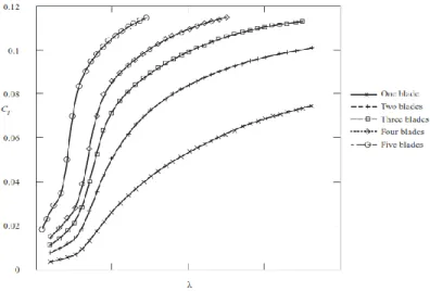
The performance of a wind turbine can be characterized by the manner in which the three main indicators (power, torque and thrust) vary with wind speed. The power determines the amount of energy captured by the rotor, the torque developed determines the size of the gearbox and must be matched by whatever generator is being driven by the rotor. The rotor thrust has great influence on the structural design of the tower. It is usually convenient to express the performance by means of non-dimensional, characteristic performance curves from which the actual performance can be determined, regardless of how the turbine is operated, e.g., at constant rotational speed or some regime of variable rotor speed. Assuming that the aerodynamic performance of the rotor blades does not deteriorate the non-dimensional aerodynamic performance of the rotor depend upon the tip speed ratio and, if appropriate, the pitch setting of the blades. It is usual, therefore, to display the power, torque and thrust coefficients as functions of tip speed ratio. [2]
𝑪𝑷− 𝝀 Performance curve
Once the blade has been designed for optimum operation at a specific design tip speed ratio (defined as the ratio between the blade tip speed and the wind speed), the performance of the
33
rotor over all expected tip speed ratios needs to be determined. For each tip speed ratio, the aerodynamic conditions at each blade section need to be defined. From these, the performance of the total rotor can be determined. The results are usually presented as a graph of power coefficient
𝐶𝑃 versus the tip speed ratio 𝜆. This graph is called the 𝐶𝑃− 𝜆 curve.
The logic behind the shape of this curve is plausible, considering that, at λ = 0 the rotor does not rotate and hence cannot draw power from the wind, while at very high λ (here at λ=12) the rotor runs so fast, that it is seen as a completely blocked disc by the wind. Wind flows around this "solid" disc, so there is no mass transport through the rotor, and thus, no possibility to extract energy from a moving mass. Somewhere between λ=0 and λ=12, there will be an optimum value (here at λ=8) for which the maximum power is extracted. This will be the condition, in which the mean velocity at the rotor disc is almost 2/3rd of the wind speed, according to the Betz law.
𝑪𝑸− 𝝀 Performance curve
The torque coefficient is derived from the power coefficient, simply by dividing it by the tip speed ratio. As a result, it gives no additional information about the turbine performance. The principal use of the 𝐶𝑸− 𝜆 curve is for torque assessment purposes when the rotor is connected
to a gearbox and generator. [2]
34
Figure 1.28 shows how the torque developed by a turbine rises with increasing solidity. For modern high-speed turbines, designed for electricity generation, as low a torque as possible is desirable in order to reduce gearbox costs. On the other hand, a high-solidity multi-bladed turbine rotates slowly and has a very high starting torque coefficient.
The peak of the torque curve takes place at a lower tip speed ratio than the peak of the power curve. For the highest solidity, shown in figure 1.28 the peak of the curve occurs, while the blade is stalled.
𝑪𝑻− 𝝀 Performance curve
The thrust force on the rotor is directly applied to the tower on which the rotor is supported and so considerably influences the structural design of the tower. Generally, the thrust on the rotor rises with increasing solidity. [2]
Figure 1.32: The effect of Solidity on Thrust
For the fault diagnosis study, a simulator that provides a rough model of a variable-speed three-bladed HAWT, within a uniform wind field is considered. This model has been applied in the benchmark model by Odgaard [1] as described in the "Introduction".
Considering the briefly-described performance curves; the rotor is a uniform wind extractor transforming kinetic energy of the wind to mechanical type at the shaft and then, into
35
electrical power by the generator. The power obtained by the rotor can be characterized by the following equation.
𝑃
𝑅=
𝜌𝐴𝑟𝐶𝑃(𝜆(𝑡),𝛽(𝑡)).𝜗𝜔(𝑡)32 (1.9)
where 𝐴𝑟 = 𝜋𝑅2 is the swept area by the rotor, 𝜌 is the density of air and 𝐶𝑃 is the power coefficient.
The two most important forces experienced by the rotor are thrust and torque. The rotor torque is a result of the lift force induced on the blades by the oncoming wind. Since ideally speaking 𝑃𝑟 = 𝜏𝑅𝜔𝑟, the rotor torque can be expressed as:
𝜏
𝑅=
𝜌𝐴𝑟𝐶𝑃(𝜆(𝑡),𝛽(𝑡)).𝜗𝜔(𝑡)32𝜔𝑟 (1.10)
As the torque coefficient 𝐶𝑞 is obtained directly from the power coefficient 𝐶𝑃, the aerodynamic torque,
𝜏
𝑅 acted upon the blades can be represented by:𝜏
𝑅=
𝜌𝜋𝑅3.𝐶𝑞(𝜆(𝑡),𝛽(𝑡)).𝜗𝜔(𝑡)22 (1.11)
The thrust force is a by-product of the interaction between the blades and the wind. This force is transferred from the blades to the nacelle and tower and is given as:
𝐹
𝑇=
𝜌𝐴𝑟𝐶𝑇(𝜆(𝑡),𝛽(𝑡)).𝜗𝜔(𝑡)32 (1.12)
Both 𝐶𝑃 and 𝐶𝑇 depend on the tip-speed ratio 𝜆 and the pitch angle 𝛽. The tip speed ratio
will be defined as:
𝜆 ≡
𝜔𝑟𝑅36
Figure 1.33: Power efficiency coefficient 𝐶𝑃 given the tip speed ratio 𝜆 and the pitch angle 𝛽
.
Figure 1.34: Thrust coefficient 𝐶𝑇 given the tip speed ratio λ and the pitch angle β
Considering that the three blades might have different 𝛽 values, a simple way to model the
aerodynamic torque can be obtained by:
𝜏
𝜔(𝑡) = ∑
𝜌𝜋𝑅3.𝐶𝑞(𝜆(𝑡),𝛽(𝑡)).𝜗𝜔(𝑡)26
1≤𝑖≤3
(1.14)
This model is valid for a small difference between 𝛽 values. However, it has been examined
37
1.4.2.2 Pitch System Model
In order to vary the angle of each blade toward the wind individually, one pitch actuator is used for each blade. The pitch actuators are placed in the hub of the wind turbine. They are driven by hydraulic servo systems, each of which can be characterized by a linear second order model [1].
𝛽̈ = 𝜔
𝑛2𝛽
𝑟𝑒𝑓− 2𝛽̇𝜔
𝑛𝜉 − 𝛽𝜔
𝑛2(1.15)
Figure 1.35: Pitch System Block
It can be shown both in the state space or Transfer Function form to be applied to the wind turbine simulator. [4]
[
𝛽̇
𝛽̈
] = [
0
1
−𝜔
𝑛2−2𝜔
𝑛𝜉
] [
𝛽
𝛽̇
] + [
0
𝜔
𝑛2] 𝛽
𝑟𝑒𝑓 (1.16) 𝛽 𝛽𝑟𝑒𝑓=
𝜔𝑛2 𝑠2+2𝜉𝜔 𝑛𝑠+𝜔𝑛2(1.17)
1.4.3 Drive Train Model
In this section, the two-mass drive train model, exploited in this project, is presented. Aerodynamic torque is transferred through the drive train to the generator via the gearbox. The gearbox scales up the rotational speed by a factor, known as the gearbox ratio, to the amount that is required by the generator. [3]
38
Drive Train Differential Equations:
{ 𝐽𝑟𝜔̇𝑟 = 𝜏𝑟 − 𝐾𝑑𝑡𝜃Δ− 𝐵𝑑𝑡𝜃̇Δ 𝐽𝑔𝑁𝑔𝜔̇𝑔 = −𝜏𝑔𝑁𝑔+ 𝐾𝑑𝑡𝜃Δ+ 𝐵𝑑𝑡𝜃̇Δ 𝜃̇Δ = 𝜔𝑟 −𝜔𝑔 𝑁𝑔 (1.18)
Considering the Schematic drawing shown in figure 1.33, the low-speed shaft has connected the rotor with the speed 𝜔𝑟 and the torque 𝜏𝑟 acting on the shaft. The Inertia of the rotor and the low-speed shaft is 𝐽𝑟.
𝐾𝑑𝑡 is the spring stiffness coefficient and 𝐵𝑑𝑡 is the viscous damping parameter of the
massless viscously damped rotational spring. The gearbox ratio is characterized by 𝑁𝑔.
At the right side, the Inertia of the gearbox, high-speed shaft and the generator is assumed as 𝐽𝑔. Generator Torque and its rotational speed are shown by 𝜏𝑔, 𝜔𝑔 respectively.
Figure 1.36: Schematic drawing of a flexible drive train
Let’s define 𝜃Δ(𝑡) as the torsion angle of the drive train and 𝜂𝑑𝑡 for the drive-train
efficiency. By ignoring both viscous frictions of low-speed and high-speed shafts (𝐵𝑟, 𝐵𝑔), the state
space model can be represented by:
[
𝝎
𝒓(𝒕)
𝝎
𝒈(𝒕)
𝜽
𝜟(𝒕)
]
̇
=
[
−
BJdtr Bdt JrNg−
Kdt Jr ηdtBdt JgNg−
ηdtBdt JgNg2 ηdtKdt JgNg1
−
1 Ng0
]
[
𝝎
𝒓(𝒕)
𝝎
𝒈(𝒕)
𝜽
𝜟(𝒕)
] + [
1 Jr0
0
−
1 Jg] [
𝛕
𝛕
𝐫(𝐭)
𝐠(𝐭)
]
(1.19)39
1.4.4 Generator and Converter Model
Given the delivered torque τg on the generator side of the drive-train and the generator efficiency ηg, the electrical power can be obtained from:
𝑃
𝑔= 𝜂
𝑔𝜔
𝑔(𝑡)𝜏
𝑔(𝑡)
(1.20)The generator torque cannot be changed instantaneously. Therefore, the relationship between the requested torque and the actual torque is represented by a first order transfer function, with frequency 𝛼𝑔𝑐 .
𝜏𝑔(𝑠) 𝜏𝑔,𝑟(𝑠)
=
𝛼𝑔𝑐
𝑠+𝛼𝑔𝑐
(1.21)
In reality, the power 𝑃g produced by the generator is controlled by adjusting the flow of
current in the rotor of the generator, which adjusts the 𝑃g,r, and as a consequence the torque τg
40
1.4.5 Wind Turbine Control system concept
The generated electrical power 𝑃𝑔 and generator speed ω𝑔 are the system outputs. The controllable inputs are the reference pitch angles 𝛽𝑖,𝑟𝑒𝑓 and generator torque 𝜏𝑔,𝑟, which are used
to control the output based on certain conditions which are primarily dependent upon the wind speed 𝜗𝜔(𝑡). The pitch angle of the blades varies by three pitch actuators, whilst the generator
torque changes by a converter. The aerodynamic thrust experienced by the blades causes the tower to sway, and thus the wind speed seen by the rotor is obtained by adding the tower velocity to the wind velocity.
In the most general sense, a wind turbine control system contains a couple of sensors and actuators and a system consisting of hardware and software which processes the input signals from the sensors and generates output signals for the actuators. [2]
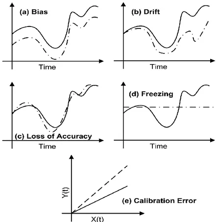
There might be various sensors, including an anemometer, a wind vane, an electrical power sensor, various limit switches, vibration sensors, temperature and oil level sensors, hydraulic pressure sensors, operator switches and push buttons.
In this study, considering the redundancy that will be discussed in chapter two and to decrease the complexity of the controller, it is assumed that the system is equipped with duplicate sensors in the following subsystems. Refer to Odgaard et al. [1], there are six sensors to measure the three pitch positions (𝛽𝑘,𝑚𝑖 , 𝑘 = 1,2,3 ; 𝑖 = 1,2), four sensors for the generator and rotor
speed measurements (𝜔𝑔,𝑚𝑖 , 𝜔𝑟,𝑚𝑖 ; 𝑖 = 1,2). It gives a total number of ten sensors, all subjected
to two different kinds of faults, including fixed value and gain factor. To be more precise, twenty faults might potentially take place.
The actuators might include a hydraulic or electric pitch actuator, sometimes a generator torque controller, generator contactors, switches for activating shaft brakes, yaw motors, etc. In this project, the considered control actuators are the three pitch systems and the converter. They allow respectively pitching the blades and setting the generator torque to control the rotational speed of the generator and the rotor.
41
The system processes the inputs to generate outputs usually consists of a computer or microprocessor-based controller which carries out the normal control functions needed to operate the turbine, supplemented by a highly reliable hardwired safety system. The safety system must be capable of overriding the ordinary controller to bring the turbine to a safe state, while a serious problem appears.
In this study, considering a nonlinear model of the wind turbine and noisy measurements, a switching control structure has been deployed. Assuming that the wind turbine operates in different regions, a switching strategy for the control system is designed that switches between various modes. In the following, all the details of a HAWT turbine controller are explained more deeply.
1.4.5.1 Wind Turbine Control Regions
Variable-speed wind turbines have four main regions of operation. A stopped turbine that is just starting up is considered to be operating in region one1. Region two is an operational mode with the objective of maximizing wind energy capture2. In the third region, the optimized produced power is kept constant3. In region four, which encompasses high wind speeds4, the turbine must limit the captured wind power so that safe electrical and mechanical loads are not exceeded [3].
1 Startup: In this region, the rotor speed is held constant at its minimum value. Pitch angle is usually held constant
at zero. As the wind speed increases, the aerodynamic efficiency and therefore the power coefficient rises towards
its maximum value. Upon reaching its maximum value, the control strategy switches to region II.
2Power optimization: By regulating the generator torque, the rotor speed increases with the wind speed to hold the
tip speed ratio constant, at its optimal value. The pitch angle is held at zero degrees. In this way the maximum power coefficient is achieved for all wind speeds within this region. When the rotor speed reaches its rated value,
controller mode is switched to satisfy the objectives of region III.
3Power reference following: This region exists since variable speed machines cannot achieve rated power at rated
rotor speed. The rotor speed is held constant at its rated value as the wind speed increases. It makes the power coefficient and the tip speed ratio to fall down. Despite this, the output power continues to rise towards rated power
as the increasing wind speed compensates for the decreasing efficiency. Upon reaching rated power, control
switches to region IV.
4 High wind speed: As the wind speed increases towards the cut-out value, the pitch of the blades increases. This
42
Figure 1.34: Reference power curve for a variable speed wind turbine
In this study, the focus is on the wind turbine normal operation zones, which are the second and the third regions [1]. For practical reasons, the transition between these zones must be done as smoothly as possible that means they might be divided into some other sub-regions.
Assuming that the wind turbine operates in region two and three, the control system switches between two different modes. In the first mode, power optimization can be achieved by setting the pitch angle to zero until the nominal power value is reached, while the target of the second mode is following the power reference in high wind speed. In this case, the generator torque is set to the rated value and blades are pitched to control the turbine angular speed, so that the power does not exceed the nominal one. In the following, all the details of a HAWT turbine controller are explained more deeply.
1.4.5.2 Wind Turbine Controller
To make the variable speed wind turbines operate in region two, the control objective is to maximize the captured energy. This means the turbine has to operate at the peak of the 𝐶𝑃(𝜆, 𝛽)
43
tip-speed ratio 𝜆 and the blade pitch 𝛽. Given R, the radius of the blades, the wind speed 𝑣𝜔 and
the angular rotor speed 𝜔𝑟, The TSR 𝜆 is defined as:
𝜆 = 𝜔𝑟. R
𝑣𝜔 (1.22)
Power coefficient 𝐶𝑃 increases the rotor power P. Therefore, operation at its maximum value 𝐶𝑃𝑚𝑎𝑥 is desirable. Note that 𝐶𝑃 can be negative, which corresponds to operating the generator as a motor while drawing power from the utility grid. The 𝐶𝑃 curve depends on the
condition of the blades, as well. For example, icing or residue buildup on the blades pushes the
𝐶𝑃 surface downward, causing the captured energy to reduce. In this project, we assumed that the blades are clean.
Figure 1.35: Power coefficient curve versus tip speed ratio and pitch for an industrial variable speed wind turbine The standard control law for operation of variable-speed turbines in region two is to let the control torque (reference torque to the converter) 𝜏𝑔,𝑟 be given by:
𝜏𝑔,𝑟 = 𝐾𝑜𝑝𝑡. 𝜔𝑟2 (1.23)
Where the gain 𝐾𝑜𝑝𝑡 is obtained from:
𝐾𝑜𝑝𝑡 =1 2𝜌𝐴𝑅
3𝐶𝑃𝑚𝑎𝑥
44
As explained above, the optimum value of the tip speed ratio 𝜆𝑜𝑝𝑡 is obtained at the peak
of the 𝐶𝑃(𝜆, 𝛽) curve, which is the maximum power coefficient. 𝜌 is the air density and A is
considered as the area swept by the turbine blades.
Apart from the converter reference signal, the pitch reference angle is held at zero degrees, in which the maximum wind speed is absorbed by the blades within this region.
𝛽𝑟𝑒𝑓 = 0 (1.25)
While the rated power is achieved (𝑃𝑔[𝑛] ≥ 𝑃𝑟[𝑛]), by setting the converter torque at the
reference value𝜏𝑔,𝑟, the controller switches to the mode corresponds to the region three. In this zone the control objective is to follow the power reference, 𝑃𝑟. This can be accomplished by controlling the blade angles β𝑘, in a manner that the power coefficient 𝐶𝑃 and the tip speed ratio
decrease to keep the generated power constant while the wind speed increases. In an industrial control scheme a PI controller is used to keep 𝜔𝑟 at the rated value by changing 𝛽𝑟.
To conclude about the control law, let’s redefine mode one as the power optimization region and the second mode as the power reference following region. The control system switches to the second mode when the condition (1.26) holds and switches back to the first mode while the condition (1.27) becomes valid, in which the rated speed of the generator decreases to some extent and pass a small 𝜔∆ threshold.
𝑃𝑔[𝑛] ≥ 𝑃𝑟[𝑛] ∧ 𝜔𝑔[𝑛] ≥ 𝜔𝑛𝑜𝑚 (1.26)
𝜔𝑔[𝑛] < 𝜔𝑛𝑜𝑚− 𝜔∆ (1.27)
The control signal (Converter reference signal) in zone two is obtained through the equations (1.23), (1.24) and (1.25). The so-called PI controller that is activated within the third region is as follows:
45
Figure 1.36: Reference Pitch angle in both regions varying with time and imposed to some faults
While the rotor speed has to reach to its nominal value by eliminating the following error through changing the pitch reference.
𝑒[𝑛] = 𝜔𝑟[𝑛] − 𝜔𝑛𝑜𝑚 (1.29)
In this case, the converter reference is used to suppress fast disturbances according to the equation (1.30):
𝜏𝑔,𝑟 = 𝑃𝑟[𝑛]
𝜔𝑔[𝑛] (1.30)