Analysis of submerged floating tunnel resting on flexible soil strata subjected to seaquake exitation

(1)

School of Civil, Environmental and Land Management Engineering

Master Degree in Civil Engineering – Structures

April 19, 2018

Analysis Of Submerged Floating Tunnel Resting

On Flexible Soil Strata Subjected To Seaquake

Excitation

Supervisor: Authors: Prof. Luca Martinelli Sara Canziani 863167 Monica Pirozzi 872288

(2)

(3)

3

List of tables

Table 1 Geometrical and mechanical characteristic of the tunnel section ... 81

Table 2 Geometrical and mechanical characteristic of the tunnel bars ... 82

Table 3 Nodes of the 2-D model midspan section ... 84

Table 4 ANSYS type element used in the 2-D model ... 84

Table 5 Nodes for the generation of ANSYS model of quarter span section ... 88

Table 6 Nodes for the generation of ANSYS model of end section ... 91

Table 7 ANSYS type element used in the 3-D model ... 94

Table 8 Values of the self-weight and buoyancy forces ... 99

Table 9 Results of static analysis for 2-D Model ... 104

Table 10 Experimental period obtain from ANSYS (TANSYS) ... 106

Table 11 Experimental frequencies obtain from ANSYS (TANSYS) ... 107

Table 12 Theoretical period (Tth) ... 107

Table 13 Natural frequencies of the 3-D model obtain from ANSYS ... 116

Table 14 Coefficients of the Soil-Structure Interaction ... 125

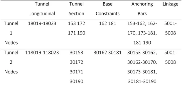
Table 15 Number of the nodes of the bars type A ... 127

Table 16 Number of the nodes of the bars type B ... 128

Table 17 Number of the nodes of the bars type C ... 128

Table 18 Added mass of the three type of bars ... 129

Table 19 Type elements used in transient analysis ... 130

Table 20 Mechanical parameters ... 146

Table 21 Characteristics of the soil strata considered ... 152

(7)

7

List of Figures

Figure 1 Typical Submerged Floating Tunnel and Suspension Bridge ... 18

Figure 2 Example of a floating tunnel with different anchoring systems. ... 20

Figure 3 SFTs with different support systems: pontoons on the surface (a); columns to the seabed (b); tensioned anchoring bars/cables to the seabed (c); support at the abutments only (d); combinations of the above methods (e). ... 22

Figure 4 Flexible soil strata on semi-infinite flexible domain ... 52

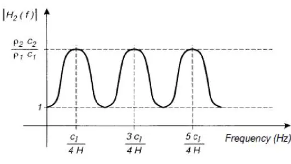
Figure 5 Amplification function of the layer overlying an elastic base ... 54

Figure 6 Schematization of rigid bedrock under a column of water d ... 55

Figure 7 Reference system ... 56

Figure 8 Characteristic parameters ... 57

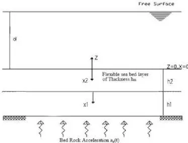
Figure 9 Schematic representation of flexible sea bed with one elastic layer ... 62

Figure 10 Schematic representation of flexible sea bed with two elastic layers ... 65

Figure 11 Fluid forces on a body ... 70

Figure 12 Unsteady moving body stationary fluid ... 71

Figure 15 Modelling of earthquake and seaquake of SFT resting on flexible layer over rigid bedrock ... 76

Figure 16 Geological model... 79

Figure 17 Transversal section of the model ... 80

Figure 18 Longitudinal section of the model ... 80

Figure 19 Tunnel section ... 82

Figure 20 Geometry of bars section ... 82

Figure 21 Code definition of the ANSYS elements used in the 2.D model ... 85

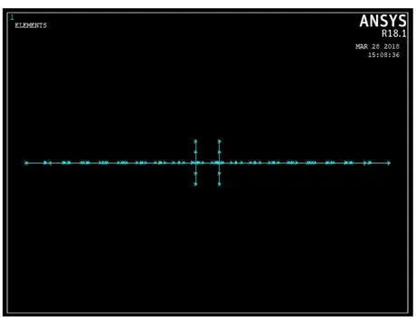
Figure 22 Frontal view of elements of the ANSYS 2-D model midspan section ... 86

Figure 23 Upper view of elements of the ANSYS 2-D model midspan section ... 86

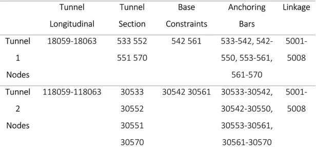
Figure 24 Nodes number of the ANSYS 2-D model ... 87

Figure 25 Nodes number of the ANSYS 2-D model ... 87

Figure 26 Transversal view of elements of quarter-span section ... 89

Figure 27 Upper view of elements of quarter section ... 89

Figure 28 Upper view of nodes of quarter span section ... 90

Figure 29 Transversal view of nodes of quarter span section ... 90

Figure 30Transversal view of elements of end section ... 92

Figure 31 Upper view of elements of end section ... 92

Figure 32 Upper view of nodes of end section ... 93

Figure 33 Transversal view of nodes of end section ... 93

Figure 34 Code definition of the ANSYS elements used in the 2.D model ... 95

Figure 35 View of the nodes of the 3-D model ... 96

Figure 36 Sectional view of the nodes of the 3-D model ... 96

Figure 37 View of elements of 3-D model ... 97

Figure 38 View of elements of 3-D Model ... 97

Figure 39 Deformed shape of the section in the 2-D model (frontal view) midspan section ... 101

(8)

8 Figure 40 Deformed shape of the section in the 2-D model (upper view midspan

section) ... 101

Figure 41 Deformed shape of the section in the 2-D model (frontal view) quarter span section ... 102

Figure 42 Deformed shape of the section in the 2-D model (upper view quarter span section) ... 102

Figure 43 Deformed shape of the section in the 2-D model (frontal view) end section ... 103

Figure 44 Deformed shape of the section in the 2-D model (upper view end section) ... 103

Figure 45 Deformed shape of the section in the 3-D model (upper view) ... 105

Figure 46 Deformed shape of the section in the 3-D model (upper view) ... 105

Figure 47 First in plane symmetric mode ... 109

Figure 48 First out of plane mode ... 110

Figure 49 Second in plane anti-symmetric mode ... 110

Figure 50 Second out of plane mode ... 111

Figure 51 Third in plane anti-symmetric mode ... 111

Figure 52 Third out of plane mode ... 112

Figure 53 Fourth in plane anti-symmetric mode ... 112

Figure 54 Fourth out of plane mode ... 113

Figure 55 Fifth in plane symmetric mode ... 113

Figure 56 Fifth out of plane mode ... 114

Figure 57 Sixth in plane anti-symmetric mode ... 114

Figure 58 Sixth out of plane mode ... 115

Figure 59 First mode of the 3-D model ... 117

Figure 60 Second mode of the 3-D model ... 117

Figure 61 Third mode of the 3-D model ... 118

Figure 62 Fourth mode of the 3-D model ... 118

Figure 63 Fifth mode of the 3-D model ... 119

Figure 64 Sixth mode of the 3-D model ... 119

Figure 65 Seaquake and Earthquake forces on the SFT ... 122

Figure 66 Rayleigh damping ... 124

Figure 67 Real section 2-D geometrical model with two bars ... 125

Figure 68 Code ANSYS definition of the used elements ... 126

Figure 69 Dampers nodes of end section ... 127

Figure 70 ANSYS code generation of the used elements ... 131

Figure 71 ANSYS code definition of parameters for Morison equation ... 133

Figure 72 Seismic force formula ... 133

Figure 73 Seaquake force formula ... 133

Figure 74 Procedure for generation of time-histories ... 135

Figure 75 Ground velocity of station 1 with a single flexible layer ... 137

Figure 76 Seaquake velocity of station 1 with a single flexible layer ... 137

Figure 77 Fourier analysis window ... 139

Figure 78 Fast Fourier Transform of seaquake velocity at station 1... 140

Figure 79 Fast Fourier Transform of ground velocity at station 1 ... 140

(9)

9

Figure 86 Seaquake velocity of station 3 with a single flexible layer ... 144

Figure 88 Seaquake acceleration power spectrum at station 3 (d = 325m) ... 145

Figure 89 Seaquake force and ground earthquake force on SFT tunnel ... 146

Figure 90 Ground velocity at station 21 for 2 flexible layers ... 147

Figure 93 Seaquake velocity at station 21 of 2 soil layers ... 148

Figure 96 Fast Fourier Transform of ground velocity at station 141 for 2 flexible strata ... 149

Figure 97 Fast Fourier Transform of seaquake velocity at station 141 for 2 flexible strata ... 149

Figure 98 Fast Fourier Transform of seaquake acceleration at station 141 for 2 flexible strata ... 150

Figure 99 Phase angles of ground velocity and seaquake velocity at station 141 with 2 flexible layers ... 151

Figure 100 Difference of phase angles of ground velocity and seaquake velocity at station 141 with 2 flexible layers ... 151

Figure 101 Vertical displacement of tunnel master node with rigid seabed for section 141 with elastic bars ... 153

Figure 102 Vertical displacement of tunnel master node with two flexible soils strata with characteristics of table 18 for section 141 with elastic bars ... 153

Figure 106 Vertical displacement of tunnel master node with two flexible soils strata with characteristics of table 18 for section 21 ... 155

Figure 108 Vertical displacement of tunnel master node with two flexible soils strata with characteristics of table 21 for section 21 ... 157

Figure 109 ANSYS code for the definition of inelastic properties of bars ... 158

Figure 110 Vertical displacement of midspan section with inelastic bars on rigid seabed ... 159

Figure 111 Vertical displacement of midspan section with inelastic bars on flexible soil strata of table 19 ... 159

Figure 112 Vertical displacement for rigid bed with elastic and inelastic bars ... 160

Figure 113 Vertical displacement for flexible layers of table 19 with elastic and inelastic bars ... 160

(10)

10

Figure 115 Schematic representation of flexible sea bed with one elastic layer ... 173

Figure 116 Schematic representation of flexible sea bed with two elastic layers .... 179

Figure 117 BEAM 4 ANSYS element ... 184

Figure 118 BEAM 188 ANSYS element ... 185

Figure 119 COMBIN14 ANSYS element ... 185

Figure 120 COMBIN39 ANSYS element ... 186

(11)

11

List of Symbols

Greek letters

 Coefficient of mass matrix

c

 Parameter controlling coherence decay

 Coefficient of stiffness matrix

t

 Ratio of the amplitude envelope at tmax

 _{Coherency function}

 _{Deterministic envelope function}

1

 First damping ratio

2

 Second damping ratio

 Damping ratio g  Ground damping f  Filter damping d

 Horizontal separation distance L

d

 Projected horizontal distance

 _{Water density}

 Fourier transform of the coherency function

 _{Random phase angles}

(12)

12

1

w First selected natural frequency

2

w Second selected natural frequency

g w Ground frequency f w Filter frequency w Circular frequency Latin letters A Section area

c Acoustic compressible wave velocity in water D

C Drag coefficient

M

C Inertia coefficient

a

C Added mass coefficient

 

C Damping matrix

d Depth of water;

D Cylinder diameter

2

x

E_ _ Mean square of the derivative of the process

g _{Gravity acceleration} ) ( ), ( ),

(g s h Superscript denoting respectively ground, structural and hydrodynamic contributions

(13)

13

( )

,

f t x Time history

)

( f Subscript indicating free-field motion

f Morison force

water

f Wave resonance frequency

k Wave number

 

K Stiffness matrix

m_add Added mass

 

M Mass matrix

n Numbers of resonance frequencies

p Peak factor

Q Generalized components of external loads vector

q _{Displacements}

R Generalized non-linear restoring forces vector

0

S Scale factor

( )

CP

S w Normalized Clough-Penzien spectrum

S PSD

max

S Peak value of the spectrum

c ,

s _{Subscript indicating structural nodes and the}

ground-structure interface

max

t Equivalent duration of the process 1 2

t，t Ramp duration and decay starting time

(14)

14 x Structure move acceleration

g( )

U t _{Vertical ground displacement at the sea bed}

u Water particle velocity

u Water particle acceleration; u x  Relative velocity

u x  Relative acceleration

s

v Shear wave velocity

app

v Surface apparent velocity of wave

V _{Section volume}

 

var x Variance (total power) of the process having PSD

water

w Wave resonance circular frequency

(15)

15

List of Abbreviations

Submerged Floating Tunnels (SFTs)

The International Tunnel Association (ITA)

The Sino-Italian Joint Laboratory of Archimedes Bridges (SIJLAB) Finite element (FE)

Bar finite element approach (NWB) Co-rotational approach (CR)

Peak ground acceleration PGA Soil structure interaction (SSI) Power spectral density (PSD) Fast Fourier Transformation (FFT) Cross-power spectral density (CPSD)

(16)

(17)

17

INTRODUCTION

Engineering is a field of study that always tries to find new challenges to face. In the Civil Engineering field, a challenge that has become popular is to cross deep-water straits or rivers of some kilometres in length with a single span bridge. Consider that the longest single span bridge ever constructed on earth is the Akashi Kaikyō Bridge situated in Japan, Kobe with a central span of 1991km (nearly 2 km).

‘2 km’ has become the new record to beat, but it is not just a matter of overcoming records, the necessity of crossing bigger spans without intermediate pillars is a necessity when the seabed is too far from the water surface and the distance to be crossed is too long, causing great conceptual and execution problems.

This is exactly the case of the Messina Strait, a piece of sea of minimum length of 3 km separating the two regions of Sicily and Calabria in Italy.

The tricky points, in this case, become two, which are strictly connected. First of all, the span of the bridge is over 1 km the maximum one ever constructed, and only this brings a lot of uncertainties and problems from the constructional point of view, besides economical aspects because a bridge of this length will have enormous costs due to the giant dimensions of the structural elements, to be constructed by special firms right on the spot or with large prefabricated pieces very difficult to move. The second aspect is the depth of the seabed, that, in some points is of nearly 300m, making impossible to realize a multi-span bridge.

At this point, the idea of the Submerged Floating Tunnel was introduced for the first time in the ’80 as an economical and convenient means to solve these types of problems, i.e. very long crossings in deep waters with a ratio cost/length quite efficient.

(18)

18

Figure 1 Typical Submerged Floating Tunnel and Suspension Bridge

The submerged floating structure is a new challenging idea still never realized that consists of a tunnel submerged in water and suspended in it or by floating islands at the sea surface or by anchoring bars at the seabed.

This type of structure is far away from the classical static structures since, being embebbed completely in water, it must exploit the effect of water, and so the Archimedes’ Force, to be sustained and should face hydrodynamic effects of various kind in case of earthquake.

The point of this work of thesis will be exactly this one: to study a Submerged Floating Tunnel subjected to seaquake excitation, i.e. the effect of the shock waves generated in water by a seismic input at the seabed. We can well understand now that, in a seismic region like the South of Italy, this is a primary design action to be considered and the seism does not excite the structure directly but passing through the “filter” of water.

We will then also consider how the seismic signal is altered passing through different layers of flexible soil before reaching the supports of the structure.

So, this work of thesis will be essentially subdivided into two parts: one more theoretical, in which all equations and mathematical aspects, motivations and descriptions will be provided and a second part, we can say, much more practical, where the model of a real case study of an SFT over the Messina Strait will be presented, implemented and then analysed first under static loads and then in dynamical conditions under the excitations of earthquake and seaquake.

(19)

19 1a) We will give a general technical explanation of what a submerged Floating Tunnel is, what are its historical developments and which are the various types of structures conceived up to this point.

1b) Then, we will focus on the seismic excitation, i.e. how to extend the given seismic input given in one point to a multiple support system, in order to be conveniently applied to the supports of our structure.

1c) Afterwards, we will introduce the concept of seaquake and its generation through the mathematical tools of transfer functions and Morison equation that enable us to transfer the seismic input from seabed to water and permitting a modelling of hydrodynamic seaquake forces on the tunnel. Then we will apply all what we have seen above in a real analysis, i.e. we will implement a finite element model with the aid of the finite element software ANSYS. The models studied are two: first we will focus on a 2-D model of a single section of the tunnel, to have a model easily controllable and fast to analyse and then we will extend it to a 3-D model.

2a) So, in a first moment, we will test the goodness of our structural model under static conditions and determine the modes of vibration of the structure. 2b) In the end, we will apply the seismic and seaquake excitations in order to determine the response of the structure under these highly variable loads. We hope you will enjoy this technical reading and we wish it will be of inspiration to you in order to produce new and interesting ideas for future developments of the problem.

(20)

20

Chapter 1: The Submerged Floating Tunnel

(SFT): a new challenging infrastructure for

crossing waterways

1.1 Introduction to SFTs

In modern civil engineering there are three conventional approaches to the solution of the water-crossing problem: bridges, underground tunnels and immersed tunnels. All of them are widely put into practice with mature design and construction technologies. Here, in this thesis, a challenging innovative structure, named Submerged Floating Tunnel (SFT) or Archimedes Bridge, is introduced as a promising alternative to cross sea-straits, lakes and waterways.

Figure 2 Example of a floating tunnel with different anchoring systems.

What are SFTs? A SFT, entirely immersed at some depth, serves all types of traffic by crossing a body of water between two shores. In most designs a circular cross section is adopted and the tunnel, subject to positive net buoyancy, is anchored at the seabed by suitable structural elements. The tunnel section is large enough to accommodate the road traffic and the related services. More generally SFTs can be fixed to the seabed, or to floating pontoons, by supporting structures spaced at intervals. Examples of these supporting structures, also called anchoring systems in this thesis,

(21)

21 are shown in Fig.2; they work in order to counteract the net buoyancy (Archimedes’ force minus weight) and to limit the tunnel motion due to environmental and operational loads.

(22)

22

Figure 3 SFTs with different support systems: pontoons on the surface (a); columns to the seabed (b); tensioned anchoring bars/cables to the seabed (c); support at the abutments only (d); combinations

of the above methods (e).

a)

b)

c)

d)

(23)

23 SFTs are suitable for long distances and deep waters. The main conditions for its competitiveness are:

 where the water depth is larger than 50 m;  where the crossing length is larger than 1 km;

 where the preservation of a scenic view or a natural habitat is considered highly important.

There are three main components in a Submerged Floating Tunnels:  Tunnel body.

It consists of one or several traffic lanes supported by a circular, elliptical or polygonal structural section; construction material is either steel, concrete or a composite combination. It is worth noting that the external diameter, and thus the volume, has a significant influence on the tunnel buoyancy.

 Anchoring system.

Pontoons on the surface, columns or other support systems from the seabed, tensioned anchor bars or cables to the seabed, support at the abutments only or combinations of the above methods. In most research work, tension element anchoring has been the first choice. There are two types of tension anchoring elements: the cables and the bars, working as a tie connection between tunnel and sea ground. The differences between them are that the bars can bear some compressive load while the cables cannot; secondly hollow-section bars can reach a straight configuration under the combined action of weight and buoyancy (neutral condition), while the cables always show a catenary-type initial shape. Hollow sections are also efficient in terms of lateral stiffness; the steel material is suitable both for high strength requirements and for good resistance to fatigue. As to the cables, they have demonstrated high reliability in bridge and offshore engineering and can be easier to be put in operation. Tension resistance can be very high.

 Shore connections.

They must satisfy two functional requirements; first, they must ensure water tightness to the joint between the floating tunnel and the onshore approaching tunnel. In structural term, the joint should be designed to allow

(24)

24 free longitudinal expansion and contraction to accommodate relative displacements between the two shores, with no vertical and transversal relative movements. The main problem for the shore connection is represented by longitudinal seismic actions; in fact, if one end is left axially free, large forces are imposed to the fixed end, also resulting in high axial forces in the tunnel section, which can be harmful for water tightness. In this work the adoption of elastic-plastic devices as longitudinal end-restraint elements has been considered, both for limiting the forces transmitted and for dissipating some of the kinetic energy developed in the tunnel. In a first design option the connection between the shore and the tunnel is left free, in axial direction, at one of the ends. At the other end a mechanical device is introduced, which should behave within the elastic range, showing high stiffness, when the axial force is smaller than the limit one. On the other hand, the device can suffer large plastic deformations when the tunnel axial force exceeds the limit value, giving rise to the hysteretic dissipative behaviour; this can be seen as an example of passive control device. In a second option, both ends are equipped with elastic-plastic devices; at one end, the device will be put in series with a shock-absorber element, allowing slow axial movements, but behaving as a rigid link when seismic actions occur.

(25)

25

1.2 History of SFTs

S. Preault first proposed the SFT idea in 1860. In 1923, the SFT was recognized as a realizable way to cross Norway fjords, whose depth is too high for bored tunnels; in fact, assuming a reasonable slope for approaching tunnel sections, a large depth results in excessive total length of the tunnel.

Then, a prize-winning proposal for a 5.3 km SFT between Calabria and Sicily over the 350 m deep Messina Strait in Italy, was proposed as an alternative to the suspended bridge. 20 years later, a remarkable time, it happened in 1989 that a working group for immersed and submerged floating tunnels was established by ITA (International Tunnel Association), which made it catch the world-wide attention [1-3], especially in Italy, Norway, China, Japan, USA and other countries.

After this notable historical moment, specialists started to work on this new topic not only on the theoretical and numerical fields but also on the design and construction aspects with growing interests. A large number of proposals were studied over the world.

In 2004, a Scientific and Technological Cooperation between the Peoples Republic of China and the Italian Republic was founded on the Sino-Italian Joint Laboratory of Archimedes Bridges (SIJLAB), which encouraged step further development on the SFTs and attracted new global interest in the topic [1-4].

Later, a prototype to be built in Qiandao Lake, an artificial lake located in Zhejiang Province, China, was proposed by SIJLAB. The prototype has a 100 m length and a 4.4 m external diameter; it was intended to be used for research purposes for some years, and then devoted to pedestrian usage and tourist attraction. Afterwards, much wider and deeper researches were based on this project. Although the project is now in a stand-by situation waiting for financial support, the obtained scientific achievements are profitable for further research or other SFTs’ proposals.

Note that, owing to the special location of the SFT, several research fields must be covered to give a thorough view on the dynamic loading and the resulting structural behaviour, such as:

(26)

26  seismic engineering analysis, studying both support-transmitted and

fluid-transmitted loads;

 fluid-structure interaction, leading to the definition of forces due to sea waves and vortex shedding;

 vehicle-structure interaction, resulting in forces due to traffic loading;

 phenomenon related to impact and explosions, applied to both internal and external events.

 geotechnical engineering, for studying the determination of the transfer functions of the seismic signal thought different layers of flexible soil strata. In seismic analysis, both the earthquake loads due to direct ground motion transmission to the structural supports and the so-called “seaquake” loading, due to the water transmission of compressive waves originated at the seabed, are worth more attention.

Oscillation due to dynamic interaction with moving vehicles is an aspect, which deserves investigation in relation to fatigue considerations and comfort requirements for people travelling through the tunnel. The latter aspect seems to be of utmost importance for an innovative infrastructure whose psychological acceptance from the community must be ensured by all technical means. There is nearly no related work on SFTs on this traffic problem, but there are similar works on other crossing solutions. From the literature review, there is limited research effort focusing on the response of SFTs subjected to the seaquake forces, transmitted from the seabed vibration to the structure through water. More attention should be paid on this research area.

(27)

27

1.3 Reasons for Choosing Floating Tunnel

As an innovative structure to be taken as an alternative to traditional waterway crossing solutions, there are some pros and cons related to the SFT concept.

The pros are for SFTs:

 they ate invisible thanks to the submerged position in the water;  take advantage of the water buoyancy;

 allow for very low gradient of the approaching lanes and thus for smaller overall tunnel length;

 provide space above the water surface for the ship traffic requirements and/or scenic view demand;

 are constructed away from densely populated areas and moved to the definite site;

 can be almost integrally removed at the end of the lifetime;  have the possibilities of reuse or recycling;

 have a cost which is only linearly proportional to length;  are theoretically feasible to surpass spans of any length;  are not subjected to the wind actions;

 are subjected to water waves in a limited way, with a lower effect if compared to the wind acting on a bridge;

 are less dependent on the mechanical soil properties than underground tunnels or immersed tunnels.

On the contrary, some of the cons are listed below:

 a SFT is an unusual structure and little experience is available in practise;  the abnormal location in the water needs more care in the safety assessment;  new structures often receive much more challenges and tests;

 the environment is complex due to its position;

 there are difficulties in the construction to position the tunnel at a definite place;

(28)

28  some accidental loading conditions involve very complex studies.

The pros shown seem to largely justify the interest on the SFT concept. On the other hand, SFTs deserves more comprehensive studies to solve some scientific and technical problems in order to convince the public of its safety. In order for the project come to fruition, various technical, economic, and social impact aspects must still be deeply investigated.

(29)

29

1.4 Design Features

The first step in the realization of a never-built structure is to have an all-round conceptual design; for a SFT this should cover the overall structural configuration, the cross-section and the supporting system of the tunnel. There are several aspects to be decided once the SFT proposal starts.

 Placement and length.

The tunnel length mainly depends on the distance of shores, but also on its placement. SFTs are considered for long crossings and as the tunnel length increases, the SFT cost will proportionally decrease when compared to other solutions. For very long tunnels, the end connections to the shore are likely to become a critical aspect of the design, especially when high seismic forces must be considered.

 Depth.

Since the SFT plays the role of ‘underground bridge’ with an anchoring system connecting it to the seabed, the water depth plays an important role. A hundred meter depth is considered a limit for column supported submerged tunnels; in deeper waters other solutions, as the one here considered, must be adopted. Another question is how deep should be placed the SFT tunnel in the water. The tunnel position in the water should leave enough space for the surface navigation; considering important sea-strait crossings, where large ships can navigate, a 30-40 m clear depth is deemed to be sufficient

Referring to the tunnel, the configuration of the tunnel cross-section and the choice of the material are the main aspects to be decided.

 Cross-section; circular.

It has a marked effect on the hydrodynamic and structural behaviour. However, it is also decided based on functional requirements; for instance, the number of lanes for cars or railroad tracks and the various types of services to be considered. The internal diameter should be enough to accommodate them and to ensure the normal required operation. The external diameter, on the other hand, has the prominent influence on the ratio between the water

(30)

30 buoyancy and the tunnel weight, which is expected to be larger than one. It was detected that the increase of the ratio from 1.25 to 1.4 can lead to impressive improvements of the SFT response to extremely severe sea states. In general, a large ratio can improve the structural performance under severe environmental loadings; it is worth noting, however, that high net buoyancy forces can result in very high tension forces on the foundations under extreme loading, this being an aspect to be carefully considered in terms of feasibility and cost. Besides that, the cross-section must have enough strength to be always kept in the elastic region in any loading condition, to avoid any type of cracking in order to meet the water tightness requirement.

 Cross-section; other shapes.

There are some different types, like circular, polygonal or elliptical, rectangular and circular tubes enclosed inside an external shell having a streamlined shape. The configuration depends on the traffic lanes and related facilities in a great measure.

 Material

In FEHRL (1996), it is mentioned that the selection of the materials to be used to build a Submerged Floating Tunnel must be made according to the structural and functional performance which are intended to be ensured, but it has also to be a compromise among several factors such as the resistance to the marine environment, fabrication, assembly and maintenance issues, time needed for the supply, material and constructional cost, et cetera. The possible materials used in tunnel are steel, reinforced concrete, pre-stressed reinforced concrete, aluminium alloys and rubber foam. The most acceptable and reasonable material, having a large and experienced application in other immersed tunnels, is the steel-concrete composite one, which has higher strength and good resistance to fatigue from the steel material, and higher resistance to the corrosion and heavy beneficial weight (especially in SFTs) from the concrete material.

(31)

31 The tunnel body will move upward because of the positive net difference between water buoyancy and tunnel weight if there were no anchoring system. Or, as to the other supporting system (with pontoons floating on the water surface, see Fig 2), the tunnel will sink down to the seabed because of dead weight. As a result, the supporting system seems essential in the preliminary design. Two different load-carrying systems, the seabed anchoring system and the pontoon, can be seen as alternatives. The latter one is only accustomed to the very calm environment. More detailed proposals are based on the seabed anchoring system, which can be provided by means of anchoring bars or cables. Until now, the anchoring bar solution seem to be more competitive in complex environment, as it will be discussed in detail. When the anchoring bars are selected, the cross-section should be made in detail. Hollow sections seem to be the best choice, for they can have almost neutral buoyancy and higher lateral stiffness efficiency. The material for the bars is steel with high strength and good resistance to fatigue, which is of common usage in offshore engineering.

(32)

32

References in Chapter 1

[1-1] Ahmet Gursoy, Parsons Brinckerhoff International, Inc Tunnelling and Underground Space Technology 12, 83-86 (1997).

[1-2] Mariagrazia Di Pilato, Dynamic behaviour of Submerged Floating Tunnels (SFT) subjected to seismic and hydrodynamic excitation, Politecnico di Milano, Dipartimento di Ingegneria Strutturale PhD thesis (2006).

[1-3] Christian Ingerslev, Immersed and Floating Tunnels, Procedia Engineering 4, 51-59 (2010).

[1-4] Håvard

ø

stlid, When is SFT competitive? Procedia Engineerin 4, 3-11 (2010). [1-5] Federico Perotti, Gianluca Barbella, Mariagrazia Di Pilato, The dynamic behavior of Archimede’s Bridges: Numerical simulation and design implications, Procedia Engineering 4, 91-98 (2010).

[1-5] Di Pilato, M., Feriani A., Perotti, F., Numerical models for the dynamic response of submerged floating tunnels under seismic loading, Earthquake Engineering and Structure Dynamics, (2008).

[1-6] Martinelli, L., Barbella, G., Feriani, A., A numerical procedure for simulating the multi-support seismic response of submerged floating tunnels anchored by cables, Engineering Structures 33, 2850-2860 (2011).

[1-7] Di Pilato, M., Perotti, F., Fogazzi, P, 3D dynamic response of submerged floating tunnels under seismic and hydrodynamic excitation, Engineering Structures, 30, 268-281 (2008).

[1-8] Youshi Hong, Fei Ge, Dynamic response and structural integrity of submerged floating tunnel due to hydrodynamic load and accidental load, Proceeding Engineering, 4, 35-50 (2010).

[1-9] Feriani A, Mulas MG and Lucchini G. Vehicle-bridge dynamic interaction: an uncoupled approach. Proc. of International Conference on Noise and Vibration ISMA 2008, Editors P. Sas, M. De Munck, Leuven, Belgium, Sept. 2008.

(33)

33 [1-10] Ahrens, D., Submerged floating tunnels: a concept whose time has arrived, Tunn. Undergr. Space Technol.11, 505-510 (1996).

[1-11] Brancaleoni F., Castellani A., D’Asdia P., The response of submerged tunnels to their environment, Engineering Structures, 11, 47-56 (1989).

[1-12] Giulio Martire, The development of Submerged Floating Tunnels as an innovative solution for waterway crossing, Facoltà di Ingegneria, Università degli Studi di Napoli Federico , PhD thesis (2010)

(34)

34

Chapter 2: Multiple-support seismic excitation

for the dynamic analysis of a SFT.

The problem that will be treated in this chapter deals with the seismic excitation to be applied to the supports of the structure.

If you consider a structure of moderate extension (we are talking about of order of meters), for example, a simple multi-story building used for residence purposes, we can study its dynamic behaviour exciting all its foundation with a single accelerogram. So we can make the approximation of having the same seismic motion for all the supports of the structure.

In the case of an SFT, due to the big distances crossed by such structure, we cannot use the same seismic input for all the supports because it is generated in a single point and then attenuated traveling from the epicentre to the point of interest. Having the supports a large distance between one another, we will have different intensity of the seismic motion in every point of the structure that we cannot neglect. Therefore, it is necessary to make reference to a non-synchronous input.

It is known that the response of an elastic structure subjected to a non-synchronous input can be obtained from the superimposition of two contributions: a dynamic component induced by the inertia forces and the so-called pseudo-static component, due to the difference in the support displacements. These latter can induce significant distortions in the structure, thus modifying the internal forces with respect to the case of synchronous input.

Therefore, the knowledge of the seismic motion time history at all the soil-structure interface nodes is required. A SFT has plan dimensions of the order of some kilometres; in this condition, a structural system must be considered to be subjected to partially correlate non-synchronous seismic input motion. In the work here described, this type of input has been introduced making use of artificial time histories.

(35)

35

2.1 Stochastic modelling of the ground motion

The stochastic modelling of the space-time variation of the seismic excitation is based on the Kanai-Tajimi power spectral density (PSD) modified by Ruiz and Penzien, which has been adopted to describe the seismic motion at a single point. In addition, the coherency model of Luco and Wong was introduced for representing the spatial variation of the ground motion. The resulting model is used for the generation of artificial time histories, which is made very efficient by introducing the Fast Fourier Transformation (FFT) method.

2.1.1 Coherency function for spatial variability: Luco and

Wong model

In long structures, it cannot be assumed that the same input ground motion will be shaking all supports. In fact, in the seismic wave propagation process three effects are responsible for the variation of the local ground motion:

 the wave-passage effect, which is the difference in the arrival times of seismic waves at different locations;

 the incoherence effect or dispersion, resulting from reflections and refraction of waves through the soil during their propagation, as well as from the different superposition pattern for waves arriving from an extended source at various locations;

 the local effect, due to the difference in local soil conditions at each location. The incoherence problem can be interpreted in terms of a random dispersion added to a reference acceleration input; the dispersion is a function of the distance between the point considered and the reference point, of the transmitting wave velocity and of a dispersion parameter. This aims to retain the acceleration response spectra of the ground motion. Due to the random character of the dispersion, the analyses are not exactly repeatable.

(36)

36 The coherency function is defined in terms of the cross-power spectral density (CPSD) of ground acceleration Si j, ( , )d w between two stations iand j at a separation

distanced. , 1/2 , , ( , ) ( , ) ( ) ( ) i j d d i i j j S w w S w S w          (2.1) where: w = circular frequency; ,( ) i i

S w ,Sj j, ( )w = PSD at the station sites.

In this work, assumeS wi i,( )S wi i,( )S w( ), there is no local effect considered, each

station is the same PSD.

The coherency function can be changed into:

, ( , ) ( , ) ( ) i j d d S w w S w     (2.2)

A suitable expression for the coherency function should reflect the phenomena. Some expressions are more designed-oriented, based on simplified methods to account for the effects of the correlation between the support motions. Luco and Wong 1986 model was here adopted in the form:

( , ) exp exp L c d d d s app w i v v                    (2.3) where: d

 = horizontal separation distance between two stations iand j; s

v = the shear wave velocity;

c

 = a parameter controlling coherence decay; L

d

 = projected horizontal distance along the wave propagation direction;

app

(37)

37 The first term on the right-hand side decays exponentially with the frequency ω, with the horizontal separation distance ξ between the two stations i and j and through the shear waves velocity vs, with the inverse of the mechanical characteristics of the soil. The second term depends on the projected horizontal distance L

d

 along the wave propagation direction and on the wave circular frequency ω, and it is a measure of the wave passage delay due to the surface apparent velocity of the waves.

The adopted model for the coherency function does not contain parameters describing the local effect, which should be accounted for in the local spectra Sii(ω). Note that in this formulation the geometric incoherence effect is given an higher weight (square power) with respect to the wave passage effect.

2.1.2 PSD Function: Modified Kanai-Tajimi Spectum of

Ground Acceleration

The adopted PSD function is the well-known modified Kanai-Tajimi spectrum of ground accelerations (Clough and Penzien 1975), expressed as (2.2)

S(w) = S S = S Ϛ

( ) Ϛ ( ) Ϛ (2.4)

where,

S = intensity of the ideal white noise process modelling bedrock acceleration; S (𝑤) = normalized Clough-Penzien spectrum;

𝑤 , 𝜁 = characteristic ground frequency and damping;

𝑤 , 𝜁 = the parameters of an additional filter introduced to guarantee finite power for displacements.

In this equation, the scale factor S0depends on the peak ground acceleration (PGA)

according to the following relation: S =

∙ ∗ (2.5)

(38)

38

p = 2 ∙ ln . ∙ ∙ (2.6)

t = equivalent duration of the process;

Ω = [ẋ ]_{[ ]} (2.7)

E[ẋ ] = mean square of the derivative of the process;

E[ẋ ] = ∫ ω S(ω)dω (2.8)

var[x] = variance (total power) of the process having PSD, S(ω).

var[x] = ∫ S(ω)dω (2.9)

var∗[x] = ∫ S (ω)dω (2.10)

2.1.3 FFT: Fast Fourier Transform Method

The Fourier Transform is an integral transform with a lot of practical applications that enables to transform a signal from the time-domain to the frequency-domain.

The general expressions of the direct F-T (from time to frequency) and the inverse F-T (from frequency to time) are the well-known formulae here below:

𝑋(𝑓) = ∫ 𝑥(𝑡) ∗ 𝑒 𝑑𝑡 (2.11)

𝑥(𝑡) = ∫ 𝑋(𝑓) ∗ 𝑒 𝑑𝑓 (2.12)

In other words, the F-T enables us to decompose a generic wave into many sub-components. More in details, the F-T allows to calculate the different components of the sinusoidal waves (amplitude, phase and frequency) that, if summed, give birth to the original signal.

This is very useful for different reasons:

1. Observing the sub-components of the wave we can filter the wave cancelling out the disturbing frequencies. After cleaning up the signal, we can bring it back to the time domain to obtain a better result.

(39)

39 2. In the frequency domain, a function of space and time can be decomposed in frequency, amplitude and phase of sinusoidal waves, so we have more information on which we can work on.

3. Working with many sinusoidal waves with different amplitude and phase is much better than working with a wave that is continuously varying in time, because in the first case we can perform the calculus with complex number that makes much easier to make certain operations that on the initial wave. The Fourier Transform is a really complex operation from the computational point of view but, in the engineering field, we use the Fast Fourier Transform to reduce the computational effort of the overall procedure.

In 1965, an algorithm called FFT (Fast Fourier Transform) has been built that, with the mechanism ‘divide et impera’, can reduce the complexity of the Fourier Transform from O(n2_{) to O(n log(n)). Practically, the FFT algorithm simplified enormously the} calculations and can be used also by small calculators. For example, if we want the Fourier Transform of 106_{points, with the FFT you can reduce the calculation time from} 2 weeks to 30 seconds.

So, with the classical transform, from time domain to frequency domain, the number of sums to be done was equal more or less to the number of points and the number of multiplications was equal to the square of the number of points. For this reason, the Fast version of the transform has been built, that enables to go to the frequency domain with much less operations, decomposing the wave into more sections and making the transform on each of them, in a fast way because the number of multiplications is drastically reduced.

The most common FFT algorithm is the Cooley-Tukey algorithm.

In our case, from the stochastic model described above, given the power spectral density and correlation function, artificial generation of time-histories has been performed by using the cosine series formula (2.13), which can be efficiently computed using the Fast Fourier Transform (FFT).

(40)

40 (x, t) = √2 ∑ _± ∑ ∑ S(k , ω )∆k∆ω / ∙ cos ηk x + ω t − + φ( ) (2.13) where:

f(k, ω) = the time history;

S(k, ω) = frequency-wave –number (F-K) spectrum; k = wave number;

𝜑( )= two sets of independent random phase angles uniformly distributed in 0, 2 . 

To use the preceding equation, a discretization of the frequency-wave-number spectrum is to be performed. The F-K spectrum is obtained as follows:

S(k, ω) = S(ω) ∙ Γ(k, ω) (2.14)

Γ(k, ω) = the Fourier transform of the coherency function, which satisfies the condition

∫ Γ(k, ω)dk = 1 (2.15)

which implies

∫ S(k, ω)dk = S(ω) (2.16)

That is, the power pertaining to a frequency is distributed among all the wave numbers. In the definition of only the geometric incoherence term is included in the F-K spectrum.

|γ(ξ , w)| = exp − (2.17)

So, we can get

Γ(k, ω) = ∫ |γ(ξ , w)|e dξ =

√ exp − | | (2.18) An advantage of equation is that the resulting F-K spectrum is quadrant symmetric S(k, ω) = S(−k, ω) = S(k, −ω) = S(−k, −ω) (2.19)

(41)

41 This permit simplifying the discretization of the spectrum. Vanmarcke (1983) first introduced the concept of quadrant symmetry. Note that coherency functions yielding quadrant-symmetric F-K spectra can depict only the incoherence of the seismic motions (Zerva 1992), and therefore the apparent propagation (wave-passage effect) of the seismic motions should be included explicitly in the equation of the simulated field, by means of the time-shiftx v/ app.

The discretization is performed within the limits of an upper cut off wave number ku

and an upper cut-off frequencywn, beyond which the contribution to the total power

can be considered as negligible for practical purposes. On the regressions on the F, M and S spectra, these can be determined as follows:

ω = 20 ∙ ω (2.20)

k = 6.65 ∙ ω . e . (2.21)

The upper cut-off frequency was determined by satisfying the following condition: ∫ ( , )

∫ ( , ) − 1 = 10 (2.22)

Whereas the upper cut -off wave number was determined by satisfying the following conditions:

S k _,ω = S ∙ 10 ; S(k , ω) = 0 (2.23) where S ≈ 2.218 = peak value of the spectrum, which occurs at the point with coordinates (k=0, ω ≈ 0.123ω ).

A way to check whether the upper cut-off frequency is correct for practical purposes is to make use of (3-a) as follows:

∑ 𝑆(𝑘, ω )∆𝑘 ≈ 𝑆(w ); 𝑤 = 0, … . . , 𝑤 (2.24) Once the cut-offs are determined, the discrete wave number and frequency are given by

(42)

42 𝑤 = 𝑛∆𝑤; 𝑛 = 0, … . , 𝐿 − 1, 𝑐𝑜𝑛 𝐿 ≥ 2𝑁 (2.26) M, L = powers of 2;

J,N = powers of 2;

J is larger or equal than the number of points for the discretization in space of the field (number of sites where the field is needed), JΔk = ku

N is larger or equal than the number of points for the discretization in time of the field (number of points in the time histories) NΔw = wu

The equation (4-11), can be rewritten to allow the usage of the fast Fourier transform (FFT) method, as f x , t , − = √2 𝑅𝑒 𝑒 , ∑ _± ∑ ∑ S(k , ω )∆k∆ω / 𝑒 ∅( ) 𝑒 / _𝑒 / (2.27) Where: 𝑥 = 𝑟𝛥𝑥 = 𝑟 ; 𝑟 = 0, … . , 𝑀 − 1 (2.28) 𝑡 = 𝑠𝛥𝑡 = 𝑠 ; 𝑠 = 0, … . , 𝐿 − 1 (2.29) As a last remark, note that the period of the simulations is

𝑇 =

∆ = 𝐿∆𝑡 ≥ 𝑁 ∆𝑡 = 𝑡 (2.30)

From the upper, the ground acceleration is expressed as a stationary process. Finally, we recall that we assumed the free-field ground acceleration to be a uniformly modulated non-stationary process. To account for the non-stationary characteristic of ground accelerations, the stationary time histories generated are modulated by means of a deterministic envelope function (t).

𝜂(𝑡) = 𝑝𝑒𝑟 0 ≤ 𝑡 ≤ 𝑡

(43)

43 𝜂(𝑡) = 𝑒𝑥𝑝 𝑙𝑛𝛽 𝑝𝑒𝑟 𝑡 ≤ 𝑡 ≤ 𝑡

where:

𝑡 , 𝑡 = ramp duration and decay starting time; 𝑡 = time-history duration;

(44)

44

2.2 Seismic Motion Modelling Parameters

In the PSD equation, required parameters are adopted in the following: ω = 10 𝑟𝑎𝑑𝑠 , Ϛ = 0.4 , ω = 1.0 𝑟𝑎𝑑𝑠 , Ϛ = 0.6

In the coherency function (3-3), the related parameters are assumed: v = 3500 𝑚/𝑠 , v = 4950 𝑚/𝑠 , 𝛼 = 1

In respect of the deterministic envelope function (3-31), the unknowns are given: 𝑡 = 2𝑠 , 𝑡 = 5𝑠, 𝑡 = 40𝑠, 𝛽 = 0.25

For the transversal and vertical directions, peak ground acceleration PGA is 0.64 g while 85% of this value is taken for the longitudinal direction.

To take account of multiple-support excitation and soil structure interaction, displacement time histories and velocity time histories are required. Based on the frequency domain procedure, double integration to get time histories of ground velocity and displacement are described in chapter 5.

(45)

45

2.3 Conclusions

We have seen here how to generate non-synchronous seismic input motion that is needed to apply the dynamic loading to the supports of the SFT. In this way, we can take into account all the modifications that the seismic input undertakes traveling from the epicentre to the various points of the structure.

In Chapter 5, you will find generation and application of the time histories here theoretically derived.

(46)

46

References in Chapter 2

[2-1] Monti et al. - 1996 - Nonlinear response of bridges under multi-support excitation [2-2] Shinozuka & Deodatis - 1996 - Simulation of multi-dimensional Gaussian stochastic fields by spectral representation

[2-3] Ray W. Clough, Joseph Penzien (1995), Dynamics of Structures, Computers & Structures, Inc.

[2.4] Fogazzi, P., Perotti, F. (2000), The dynamic response of seabed anchored floating tunnels under seismic excitation, Earthquake Engng Struct. Dyn. 29, 273-295.

[2.5] Martinelli L., Barbella G., Feriani A. (2010), Multi-support seismic input and response of submerged floating tunnels anchored by cables, Technical Report N.6/2010, Università degli Studi di Brescia.

(47)

47

Chapter 3: The Concepts of Seaquake and

Transfer Function

3.1 What is Seaquake

Seaquake is a hydrodynamic pressure propagating through water due to the seismic waves generated by an earthquake with epicentre beneath the sea. This phenomenon causes hydrodynamic excitations on the submerged structures.

The point is to understand If these forces provide a positive contribution to the overall behaviour of the structure, and so they tend to uplift the tunnel, or they provide a negative contribution, tending to make the tunnel sink.

3.1.1 Generalities

With the recent developing trend towards the exploitation and utilization of the ocean space, more and more projects involving floating structures are proposed and catch a lot of attention in the engineering research field. With regards to their special location, it is necessary and essential for the designers and researchers to ensure structural safety with respect to all types of hydrodynamic excitation, including the ones due to the so-called seaquake phenomenon. Actually, a number of cases call for attention to the effects of propagating seismic waves in water due to seaquakes and to the potential damaging effects that such waves may cause on the offshore structures and floating systems. These considerations hold for a new challenging structure as a SFT, submerged in the middle of the ocean. What is a seaquake will be the primary task to make it clear. It is defined as a hydrodynamic pressure due to shock waves consisting solely of compressional waves, since water cannot transmit a shear wave, traveling through the water and excited by the motion of the seabed during an earthquake. As an environmental external accidental force acting on the structure, there were few studies on this topic. Rudolph (1887, 1895) was the first to study the phenomenon and gives an extensive list of occurrences. In 1957, Richter discussed further observations of the effects of earthquakes on the surface ships and submarines. In 1981, Hove

(48)

48 presented some cases of ships being severely shaken by seaquakes. One of them, considered as the most serious, concerned MT ‘ Ida Knudsen’, a 32,500 ton Norwegian tanker that was struck by a magnitude 8.0 event on February 28, 1969 in the Atlantic Ocean approximately 450 km west of Gibraltar, and which damage was classified as total loss after an extreme shaking coming from beneath. Then, in 1983, Arochiasamy did some studies on the nonlinear transient response of floating platforms to the seaquake-induced excitation including cavitation effects. In 1988, Gin-show Liou proposed a systematic numerical approach for the response of tension-leg platforms, studied as rigid bodies under the forces due to vertically propagating waves caused by spatially varying seismic motion of the sea-bed. In the same period, Okamoto and Sakuta proposed a mathematical approach for studying seaquakes as a propagation phenomenon of acoustic waves in compressible fluids. In 1995, Tokuo Yamamoto worked on the stochastic fluid-structure interaction of large circular floating islands subject to wind waves and seaquakes and on the harmonic propagation of gravity waves and acoustic waves in the sea due to the vertical oscillation of the seabed. In 2002, Yoshiyuki built a realistic model of the seaquake effect in time domain, considering the sea bottom slope and soft sediments. It was noted that the maximum stress responses may exceed the admissible values due to the sea shock load. A very large floating structure placed in the shallow water was studied by Takamura et al, focusing on the resonance phenomena and considering the interrelationship between the vibration of the floating structure and the deformation of the seabed; the proposed procedure was based on a new boundary integral equation in which the seabed is a semi-infinite homogenous elastic solid.

Hereafter, we will discuss the concept of transfer function as a means to determine accelerations and velocities at the top of a series of flexible layers and in water. Then, the application of seaquake forces on a SFT is described with the aid of Morison equation.

(49)

49

3.2 The Concept of Transfer Function

In order to derive acceleration and velocities in every point of the soil and water above the rigid bedrock, it is necessary to introduce the concept of transfer function.

This function can be regarded as a sort of amplification factor of the movement at bedrock that can be used to amplify the base acceleration ag and determine the dynamic characteristics of the means interested (flexible soil layers overlying the rigid bed and water).

To get an idea of the form that can assume this mathematical function, let’s consider a soil layer over a semi-infinite bedrock domain. The aim is to derive a function that can be multiplied to the movement at the bedrock to obtain the one in layer 1. The total displacement at a generic point of a semi-infinite domain in case of an incident harmonic wave can be obtained in the following way.

The problem is described by the classical 1D propagation wave equation:

=

(3.1)

where α is the speed of propagation of the wave, and the general solution has the form:

𝑢(𝑥, 𝑡) = 𝑓 (𝑥 − 𝛼𝑡) + 𝑓 (𝑥 + 𝛼𝑡) (3.2)

i.e. it is composed by the sum of two differentiable functions, that represent the incident and the reflected waves.

If we assign a wave propagating with a finite speed c from +∞ towards the origin, this wave is defined incident wave:

𝑢(𝑥, 𝑡) = 𝑓 𝑡 + (3.3)

The stress-free boundary condition associated with the free surface of the domain, yields the following (von Neumann’s type) condition named “free-surface”:

( , )

(50)

50 Substituting the general solution of the wave equation

𝑢(𝑥, 𝑡) = 𝑓 𝑡 + − 𝑔 𝑡 − (3.5)

Into the free surface boundary condition, we obtain:

𝑓 (𝑡) − 𝑔 (𝑡) = 0 (3.6)

from which g(t) = f(t) + constant. It is, however, immediate to see that the latter constant must vanish. It follows also that g(t – x/c) = f(t – x/c) represents the waveform ur_{generated by the total reflection from the free surface and propagating in the} opposite direction of the incident wave f(.). The total displacement at a generic point x is given by:

𝑢(𝑥, 𝑡) = 𝑢 + 𝑢 = 𝑓 𝑡 + + 𝑓 𝑡 − (3.7) i.e. the sum of an incident and a reflected wave.

From which it follows:

𝑢(0, 𝑡) = 2𝑓(𝑡) = 2𝑢 (3.8)

That is the amplitude of the displacement at the free surface is twice that of the incident wave.

Equation (3.7), that expresses the total displacement at a generic point of the semi-infinite domain in case of incident harmonic wave, can also be written as follows: 𝑢 = exp 𝑖𝜔 𝑡 + + exp 𝑖𝜔 𝑡 − = 2exp (𝑖𝜔𝑡)cos (𝐾𝑥) (3.9) where

𝐾 = 𝜔 𝑐⁄

with

𝑅𝑒[𝑢] = 2 cos(𝜔𝑡) cos(𝐾𝑥)

This equation shows that the half-space oscillates in stationary state of vibration for any value of the frequency of the incident wave.

(51)

51 If the semi-infinite domain is replaced by a layer of thickness H resting over an infinitely rigid base, and a sinusoidal motion of amplitude 𝑒( )_{is applied to the rigid base, the} response of the elastic layer (which is a linear system) will also be sinusoidal with a frequency ω equal to the excitation frequency Ω. In general, this response can be expressed as the sum of two waveforms propagating in two opposite directions with amplitude A and B to be determined.

𝑢 = 𝐴𝑒𝑥𝑝 𝑖𝛺 𝑡 + + 𝐵𝑒𝑥𝑝 𝑖𝛺 𝑡 − (3.10)

From the free surface boundary condition, if follows immediately that A = B, and thus

𝑢(𝑥, 𝑡) = 2𝐴𝑐𝑜𝑠 exp(𝑖𝛺𝑡) (3.11)

For x = H, the displacement must be equal to the one prescribed, namely: 𝑢(𝐻, 𝑡) = 2𝐴𝑐𝑜𝑠 exp(𝑖𝛺𝑡) = exp(𝑖𝛺𝑡) (3.12) That yields:

𝐴 = 2 cos 𝛺𝐻 𝑐 (3.13)

That substituted in equation (3.12) gives:

𝑢(𝑥, 𝑡) = exp(𝑖𝛺𝑡) (3.14)

It follows from eq. (3.14) that:

𝑢(0, 𝑡) = ( )= ( , ) (3.15) The expression

( )

=

= 𝐻 (𝛺)

represents the ratio between the displacement at the free surface and that at the bottom of the layer of arbitrary excitation frequency Ω; this ratio is called the rigid base transfer function of the layer.

(52)

52 In addition, we will now consider the case of stationary oscillations of an elastic layer of thickness H overlaying a semi-infinite domain that is also elastic. Let c1 and c2 denote the generic elastic propagation speeds in the layer and in the semi-infinite domain, respectively, ρ1 and ρ2, the corresponding mass densities, and u1(x,t), u2(ξ,t) the associated displacements.

Figure 4 Flexible soil strata on semi-infinite flexible domain

In addition to the free surface boundary condition, the continuity of stress and displacement must hold at the layer interface, namely:

𝑢 (𝐻, 𝑡) = 𝑢 (0, 𝑡) (3.16)

𝜌 𝑐 ( , )= 𝜌 𝑐 ( , ) (3.17)

The motion in the lower domain will result from the superimposition of the incident harmonic wave, whose amplitude C is assumed known, and of a reflected wave, that is:

𝑢 = 𝐶𝑒𝑥𝑝 𝑖𝜔 𝑡 + + 𝐷𝑒𝑥𝑝 𝑖𝜔 𝑡 − (3.18)

In the same way, by introducing in the layer both an upward and a downward (reflected) wave of amplitude A and B, respectively, it is found in analogy with equation (3.14)

𝑢 = 2𝐴𝑐𝑜𝑠 exp(𝑖𝜔𝑡) (3.19)

(53)

53

2𝐴𝑐𝑜𝑠 = 𝐶 + 𝐷 (3.20)

Whereas from equation (3.17) it follows

−2𝐴𝜌 𝑐 sin = 𝑖 𝜌 𝑐 (𝐶 − 𝐷) (3.21)

From which, by setting η = ρ2*c2/ρ1*c1 one obtains

i2Asin = 𝜂(𝐶 − 𝐷) (3.22)

Dividing the sides of (3.22) by η and summing up (3.20) and (3.21) gives

𝐴 = (3.23)

Whence, substituting into eq. (3.21)

𝐷 = 𝐶 (3.24)

Since the amplitude C of the incident wave is known (one could set C=1), we can compute the unknown amplitudes of the remaining waves in the layer and in the semi-infinite domain. Note that:

𝑢 (0, 𝑡) = 2𝐴𝑒𝑥𝑝(𝑖𝜔𝑡) 𝑢 (𝐻, 𝑡) = 𝑢 (0, 𝑡) = (𝐶 + 𝐷) exp(𝑖𝜔𝑡) = 2𝐴𝑐𝑜𝑠 𝜔𝐻 𝑐₁ exp (𝑖𝜔𝑡) from which 𝐻 (𝜔) = ( , ) ( , )= (3.25)

As for the previously treated case of the elastic layer over a rigid base.

If the layer didn’t exist, the displacement u(0,t) at the surface of the outcropping base will be obtained from eq. (3.18) and by imposing the free surface boundary condition. The latter provides the equality C = D, from which