DOTTORATO DI RICERCA INTECNOLOGIAAERONAUTICA ESPAZIALE CICLO XXVII
Gravity and geodesy of the Jovian system
bodies with the Juno and JUICE missions
Candidate: Advisor:
Marzia Parisi Prof. Luciano Iess
Tutor:
Prof.Paolo Gaudenzi
I want to thank my advisor Professor Luciano Iess and all my col-leagues from the Radio Science Laboratory for guiding me during the last four years.
Dr. Yohai Kaspi, Dr. Eli Galanti and Dr. Ravit Helled for their support during my visit in Israel.
My parents Francesco and Rosetta, my sister Maria Alessandra, my grandmother Maria and my whole family, Gabriele, my best friends Marta and Marzia, for loving me and for putting up with me.
Contents ii
List of Figures vi
List of Tables xii
Abstract xv
Introduction xvi
1 Juno and JUICE disclose Jovian system’s mysteries 1
1.1 The Juno mission . . . 1
1.1.1 Scientific objectives . . . 2
1.1.2 Launch, trajectory and orbit around Jupiter . . . 3
1.1.3 The spacecraft . . . 4
1.1.4 Payload . . . 7
1.2 The JUICE mission . . . 9
1.2.1 Scientific objectives . . . 9
1.2.2 Launch, trajectory and tour of the satellite system . . 10
1.2.3 The spacecraft . . . 13
1.2.4 Payload . . . 17
1.3 Planetary targets of the gravity experiments . . . 20
1.3.1 Jupiter . . . 21
1.3.2 Ganymede . . . 23
1.3.3 Callisto . . . 25
1.3.4 Europa . . . 27
1.4 Radio science experiments . . . 28
1.4.2 Ground segment . . . 32
1.4.3 Media Calibration system . . . 35
2 Basic principles of geophysics 36 2.1 Harmonic representation of the gravity field . . . 36
2.1.1 Gravitational potential and spherical harmonics . . . 37
2.1.2 Normalization . . . 38 2.1.3 Low-degree harmonics . . . 39 2.1.4 Kaula’s rule . . . 41 2.2 Tides . . . 41 2.2.1 Tidal potential . . . 44 2.2.2 Love numbers . . . 46 2.2.3 Eccentricity tides . . . 47
2.3 Introduction to thermal wind balance . . . 51
2.3.1 Eulerian and Lagrangian viewpoints . . . 52
2.3.2 Equations of motion for fluids . . . 53
2.3.3 Hydrostatic balance . . . 55
2.3.4 Incompressible flows . . . 56
2.3.5 Equations of motion in a rotating reference frames . . 56
2.3.6 Geostrophic and thermal wind balance . . . 58
3 Orbit determination 63 3.1 Introduction . . . 63 3.2 Observables . . . 66 3.2.1 Two-way range . . . 66 3.2.2 Two-way range-rate . . . 68 3.3 Mathematical formulation . . . 70 3.3.1 Linearization . . . 70
3.3.2 Weighted Least Square solution with a priori informa-tion . . . 73
3.3.3 Estimate propagation . . . 77
3.4 Multiarc method . . . 77
4 Dynamical model and simulation setup 81 4.1 Simulation process . . . 81
4.2.1 Gravitational accelerations . . . 83
4.2.2 Planetary rotation model . . . 88
4.2.3 Non-gravitational accelerations . . . 88
4.2.4 Simulated trajectories . . . 96
4.3 Sources of noise on radiometric measurements . . . 99
4.3.1 Instrumental noise . . . 99
4.3.2 Propagation in the medium . . . 102
4.3.3 Calibration of the propagation noise . . . 105
4.4 Data Simulation . . . 107
4.4.1 Juno . . . 107
4.4.2 JUICE . . . 108
4.5 Estimation process . . . 109
5 Juno: the gravitational signature of Jupiter’s winds 111 5.1 From Cassini data to a model for Jupiter’s wind speed . . . . 112
5.2 A model of Jupiter’s density anomalies . . . 117
5.2.1 2-D model: purely zonal winds . . . 119
5.2.2 3-D model . . . 125
5.3 From density anomalies to gravity . . . 129
5.4 Estimation setup for the Juno gravity experiment . . . 133
5.5 Estimate of Jupiter’s gravity field: detection of mass anoma-lies produced by winds . . . 137
5.5.1 Shallow-wind case . . . 137
5.5.2 Mid-deep wind case . . . 141
5.5.3 Very-deep wind case . . . 146
6 Numerical simulations of the JUICE gravity experiment 151 6.1 Satellite ephemeris update . . . 152
6.2 Satellite tides . . . 152 6.3 Ganymede . . . 153 6.3.1 Estimation setup . . . 154 6.3.2 Estimation results . . . 155 6.4 Callisto . . . 168 6.4.1 Estimation setup . . . 169 6.4.2 Estimation results . . . 171
7 Conclusions and Discussion 184
1.1 Artist concept of Juno and Jupiter. Image credit: NASA/JPL-Caltech. . . 2 1.2 Juno trajectory during cruise (2011-2016). Image credit:
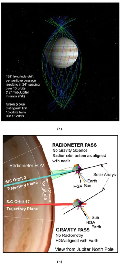
NASA/JPL-Caltech. . . 4 1.3 a)Juno science orbits around Jupiter. Image credit:
NASA/JPL-Caltech. b) Juno attitude during science observations through orbits 3-33 (Grammier, 2009). Image credit: NASA/JPL-Caltech. 5 1.4 Juno view inside the vault (Grammier, 2009). Image credit:
NASA/JPL-Caltech. . . 6 1.5 JUICE orbit insertion around Jupiter (JOI). The image also
shows the orbits of the Galilean satellites (ESA, 2011). Image credit: ESA. . . 11 1.6 Ground tracks of the Europa flybys (ESA, 2011). Image credit:
ESA. . . 12 1.7 Coverage of Callisto surface after 20 flybys. The closest
ap-proaches are divided into two groups around two different longitudes. Conventionally, for Galilean moons, 0◦ longi-tude indicates the side facing Jupiter. Different colors in-dicate different Sun elevation of the sub-nadir point (ESA, 2011). Image credit: ESA. . . 12 1.8 Artistic view of Ganymede and the spacecraft (ESA, 2011).
Image credit: ESA. . . 14 1.9 Spacecraft configuration as seen in solution 3. The +Z
di-rection represents the nadir didi-rection. (ESA, 2011). Image credit: ESA . . . 15
1.10 Fluence spectrum of electrons, divided by mission phases.
(ESA, 2011). Image credit: ESA. . . 16
1.11 JUICE payload configuration (ESA, 2011). Image credit: ESA. 20 1.12 Jupiter with the visible Great Red Spot. Image credit: NASA. 21 1.13 View of Jupiter’s interior. Image credit: Burkhard Militzer at University of California, Berkeley. . . 23
1.14 View of the interior structure of Ganymede. Image credit: NASA. . . 24
1.15 View of the interior structure of Callisto. Image credit: NASA/JPL-Caltech. . . 26
1.16 View of the interior structure of Europa. Image credit: NASA/JPL-Caltech. . . 28
1.17 Triple-link configuration of the Ka-band transponder (ESA, 2011). . . 30
1.18 The Ka-band transponder (Thales, 2012). Image credit: Thales Alenia Space. . . 31
1.19 DSN subsystems (Kliore et al., 2004). . . 33
1.20 DSA diagram (ESA, 2013b). . . 34
2.1 Spherical coordinates. Image credit: SEOS Project. . . 37
2.2 Visualization of low-degree spherical harmonics. . . 40
2.3 Tidal effects on the perturbed body. (Bertotti et al., 2003). . . 43
2.4 Tidal displacement. Image credit: David J. Stevenson, Notes of Planetary Structure and Evolution, California Institute of Technology. . . 43
2.5 Offset angle between the tidal bulge of the satellite and the line through the centers of the perturbing and perturbed bod-ies. . . 50
2.6 Components of the fluid velocity in spherical coordinates (Weisstein, Eric W. Spherical coordinates. From MathWorld, A Wolfram Web Resource). . . 55
2.7 Geostrophic (anti) clockwise flow around (low) high pres-sure regions. Explanatory image for the Earth rotation. Im-age credit: UCI Edu ESS124. . . 60
2.8 Mechanism of thermal wind for an atmospheric layer be-tween 700 and 1000 hPa. Image credit: B. Geerts, University of Wyoming, Dep. of Atmospheric Science. . . 62 3.1 Differences between estimated, true and nominal
trajecto-ries. ρ, ˙ρ and θ represent range, range-rate and angular ob-servations, respectively. Image credit: Tapley, 2004. . . 65 4.1 Block diagram of the simulation process, from the
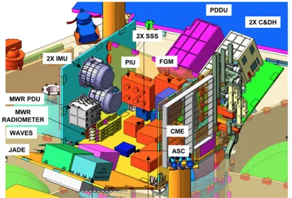
defini-tion of the dynamical model to the simuladefini-tion of synthetic tracking data. Image credit: JPL/Caltech for the Juno space-craft; ESA for the JUICE spacespace-craft; NASA for the Jupiter system; JPL Robotics for the Aerocapture Systems Defini-tion; NASA/JPL for the Galieleo trajectory; University of Wisconsin for Juno Doppler tracking. . . 82 4.2 The Juno spacecraft. Image credit: NASA. . . 88 4.3 Sketched model of the JUICE spacecraft, dimensions are given
in mm. Image credit: ESA. . . 91 4.4 Plots from Marconi (2007). Column density of Ganymede’s
atmosphere with respect to subsolar latitude (a). Density at 90◦subsolar latitude with respect to the altitude over Ganymede’s surface (b). . . 95 4.5 Juno science orbits around Jupiter. The size of the orbits and
Jupiter is to scale. . . 96 4.6 JUICE ground tracks over Callisto’s surface around closest
approach (±4h). . . 98 4.7 Altitude of the JUICE spacecraft over Ganymede during the
orbital phase. The separation between the 500-km altitude and 200-km altitude phases is evident. . . 98 4.8 Ground station elevation angle (MeteoTrentino.it). . . 104 4.9 Power spectral density of one-way plasma fluctuations.
Im-age credit: Asmar, 2005. . . 106 4.10 Doppler residuals of the Cassini solar conjunction
experi-ment in 2002 at 300s integration time. Image credit: Asmar, 2005. . . 107 4.11 Orbit determination: flow diagram of the estimation process. 110
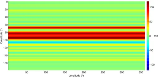
5.1 Horizontal components of the wind velocity a) u (θ, φ) com-ponent, along parallels. b) v (θ, φ) comcom-ponent, along merid-ians. The velocity map is derived from Choi and Showman (2011). . . 113 5.2 Visualization of a 2-D smoothing (e.g. over latitude and
lon-gitude). . . 115 5.3 Velocity profile over a longitudinal section (φ = π). a) for
H = 300km; b) for H = 3000km; c) for H = 1000000km. . . . 116 5.4 Spherical coordinates in the 3-D space (math.stackexchange.com).118 5.5 Surface velocity map for the zonal case. Display of the v
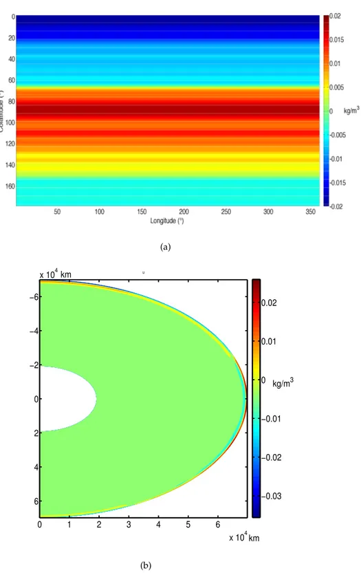
component. . . 120 5.6 Integrated density profile for H = 300km. a) Surface density
anomalies; b) Density anomalies over a longitudinal section, at φ = π. . . 122 5.7 Integrated density profile for H = 3000km. a) Surface
den-sity anomalies; b) Denden-sity anomalies over a longitudinal sec-tion, at φ = π. . . 123 5.8 Integrated density profile for H = 1000000km. a) Surface
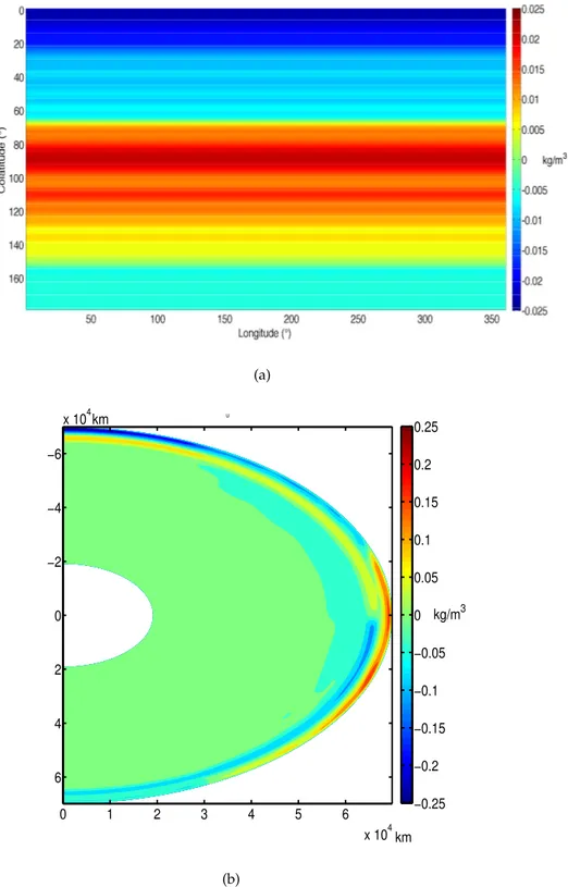
density anomalies; b) Density anomalies over a longitudinal section, at φ = π. . . 124 5.9 Integrated 3-D density profile for H = 3000 km at the surface
of Jupiter. . . 129 5.10 30x30 gravity field of Jupiter. Each box indicates a specific
tesseral harmonic of degree l and order m. a) for H = 300 km; b) for H = 3000 km; c) for H = 1000000 km. . . 132 5.11 Gravitational signature of the thermal winds. a) for H = 300
km; b) for H = 3000 km; c) for H = 1000000 km. . . 134 5.12 Zonal gravity field of Jupiter in terms of harmonic
coeffi-cients (degree 2 to 30) and associated a priori uncertainties. . 136 5.13 Gravity anomalies due to thermal winds, for H = 300 km. a)
estimated anomalies; b) formal uncertainties (1σ, logarith-mic scale). . . 139 5.14 Estimation errors versus formal uncertainty (1σ). . . 140 5.15 Ratio of the gravitational signal of the anomalies and
5.16 Gravity anomalies due to thermal winds, for H = 3000 km. a)estimated anomalies; b) formal uncertainties (1σ, logarith-mic scale). . . 143 5.17 Estimation errors versus formal uncertainty (1σ). . . 144 5.18 Ratio of the gravitational signal of the simulated anomalies
to associated formal uncertainties (1σ). . . 144 5.19 Estimated gravity anomalies after the removal of the mean
field along the longitude direction. . . 145 5.20 Ratio of the gravitational longitudinal oscillations of the
es-timated anomalies and associated formal uncertainties (1σ). 146 5.21 Gravity anomalies due to thermal winds for H = 1000000 km.
a)estimated anomalies; b) formal uncertainties (1σ, logarith-mic scale). . . 147 5.22 Estimation errors over formal uncertainty (1σ). . . 148 5.23 Ratio of the gravitational signal of the estimated anomalies
to associated formal uncertainties (1σ). . . 149 5.24 Ratio of the gravitational longitudinal oscillations of the
es-timated anomalies and associated formal uncertainties (1σ). 150 5.25 Enlargement of Figure 5.24 near the GRS location. . . 150 6.1 Visual display of Kaula’s rule for Ganymede’s gravity field.
Estimated coefficients for Ak = 2, 20, 200(blue, orange, green line), formal uncertainties (black solid/dashed line, σ/3σ level) and estimation errors (red line). . . 157 6.2 Correlation matrix for global parameters. . . 158 6.3 Gravity disturbances over the reference ellipsoid of Ganymede.
Central values (a); formal uncertainties (b); estimation errors (c). . . 160 6.4 Geoid heights over the reference ellipsoid of Ganymede.
Cen-tral values (a); formal uncertainties (b); estimation errors (c). 161 6.5 Doppler residuals of range-rate measurements at Ganymede,
from February 22, 2033 to July 4, 2033. . . 162 6.6 Convergence of the estimation process of Ganymede’s tidal
Love number, real and imaginary components, to the simu-lated value, after 4 iterations. (a) k2<; (b) k2=. . . 164 6.7 Ganymede’s GM estimate: output of the multi-arc filter. . . . 166
6.8 Accuracies in the determination of the spacecraft position. Radial component (blue line); across-track component (red line); along-track component. . . 167 6.9 Estimation results for the gravity field of Callisto. (a)
unnor-malized degree-2; (b) unnorunnor-malized degree-3. . . 173 6.10 Callisto science phase: numerical simulations. Correlation
matrix for the global parameters. . . 174 6.11 Gravity disturbances over the reference ellipsoid of Callisto.
Formal uncertainties (a), the black lines represent JUICE ground tracks over the satellite surface; estimation errors (b). . . 175 6.12 Geoid heights over the reference ellipsoid of Callisto, in terms
of formal uncertainties. . . 176 6.13 Doppler residuals of range-rate measurements at Callisto,
for all 20 flybys. Spacecraft tracking from: Goldstone (green dots); New Norcia (purple dots); Cebreros (blue dots). . . 177 6.14 Distribution of Callisto flybys in terms of satellite mean anomaly
(M). . . 178 6.15 Convergence of the estimation process of Callisto’s tidal Love
number, real component, to the simulated value, after 4 iter-ations. . . 178 6.16 Callisto’s GM estimate: output of the multiarc filter. . . 179 6.17 Estimation accuracy of Callisto tidal Love number attainable
with a different number of flyby (at the best combination). . 183 7.1 Ratio of the gravitational signal to the formal uncertainty at
the Great Red Spot location, for different values of H. The black triangles represent the analysis results. The red line represents the lower bound on the SNR. . . 185
1.1 Juno payload (Grammier, 2009 and Bolton, 2010). . . 8
1.2 Ganymede science phase: sub-phases. . . 13
1.3 JUICE payload (ESA, 2011), (ESA, 2013a). . . 19
1.4 KaT Technical Typical Performance (Thales, 2012). . . 31
1.5 DSA technical profile (ESA, 2013b). . . 34
2.1 Inclination and eccentricity of the orbits of the Galilean satel-lites with respect to Jupiter’s equator (”Planetary Satellite Mean Orbital Parameters”. Jet Propulsion Laboratory, Cal-ifornia Institute of Technology). . . 49
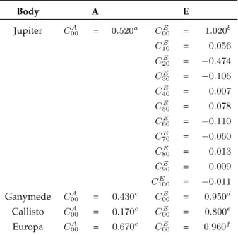
4.1 Jupiter’s un-normalized even zonal harmonics. aJacobson (2003). . . 84
4.2 Low-degree un-normalized spherical harmonic coefficients for the gravity fields of Ganymede, Callisto and Europa from Galileo gravity data (Bagenal, 2004). µ is the correlation co-efficient. . . 85
4.3 Normalized simulated full 30×30 zonal gravity field of Ganymede (weak case) plus tidal Love numbers. . . 86
4.4 Un-normalized simulated 3x3 gravity field for Callisto. . . . 87
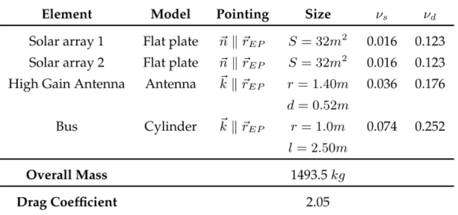
4.5 Summary of the geometric properties of the Juno spacecraft components. ~n is the normal unit vector, S is the overall surface, ~k specifies the axis direction, r is the radius, d is the depth and l is the length. The information has been retrieved from the Juno Launch Press Kit. . . 89
4.6 Optical properties adopted for the Juno spacecraft model. For the solar panels and the other components, SMART-1 like and Cassini-like properties have been adopted, respec-tively. . . 90 4.7 Summary of the geometric properties of the JUICE
space-craft components. . . 90 4.8 Planetary radiation coefficients. aJupiter albedo coefficients
for the Juno orbit determination (Finocchiaro, 2013);bJupiter thermal emission coefficients for the Juno orbit determina-tion (Finocchiaro, 2013); cYeomans (2006); dSpencer et al., 1983;eBurgdorf et al., 2000;fMarshall et al., 2011. . . . 93 4.9 Information about the geometry of the ground tracks at the
epochs of pericenters. The latitude and longitude of the C/As are given with respect to Jupiter body-fixed reference frame. αis the angle between the line of sight and the orbital plane. 97 4.10 Summary of the link budget for a space mission at Jupiter.(a)
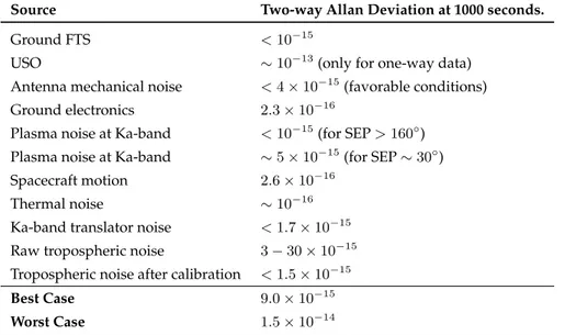
Slobin, 2012;(b) ESA, 2013b;(c)TAS-I;(d) Simone et al., 2009. Values of other parameters, such as the power transmitted by the JUICE spacecraft, have been arbitrarily, yet coherently, selected. . . 101 4.11 Allan deviations for the main noise sources on range-rate
measurements (Asmar, 2005). . . 108 5.1 Contributions to the zonal harmonics due to the winds of
Jupiter, up to degree 10. The coefficients are unnormalized. Top left: for H = 300 km; Top right: for H = 3000 km; Bottom: for H = 1000000 km. . . 130 6.1 Observation schedule for the Ganymede orbital phase. . . . 153 6.2 Initial values for the mass and quadrupole gravity field of
Ganymede. Spherical harmonic coefficients whose initial con-ditions are not shown are initialized to null. . . 154 6.3 Estimation results for unnormalized Ganymede’s zonal
6.4 Convergence of Ganymede’s tidal Love number, real and imaginary components, to the simulated value, after 4 itera-tions. . . 163 6.5 Relevant information on Callisto flybys. The flyby
nomen-clature is consistent with the one set by ESA. . . 169 6.6 Initial values for the mass and quadrupole gravity field of
Callisto. All other gravity coefficients whose initial condi-tions are not shown are initialized to null. . . 170
The key to the understanding of our Solar System, how it originated and evolved, lies with the exploration of the miniature system of its largest planet, Jupiter. To this end, a number of space missions have been dedi-cated to probing the planet itself and its satellites, aiming at studying and comprehending the physical phenomena taking place within the system. In this context, a fundamental role is played by the determination of the grav-ity field of the bodies forming the system, by means of onboard radio sci-ence experiments. The main purpose of my research is to assess the accura-cies attainable with the gravity measurements performed by NASA’s Juno and ESA’s JUICE missions, that will influence the comprehension of the in-terior structure and dynamics of the Jovian system bodies. In the frame of this dissertation I show how the precise reconstruction of the gravitational potential of Jupiter and its largest moons have the potential of improving our knowledge of the geodesy of the whole system.
Jupiter had been known to humanity since ancient times, while the Galilean moons, the largest in the system, were first observed by Galileo Galilei in 1610, using a telescope. Half a century later, Giovanni Domenico Cassini discovered that Jupiter appeared oblate and noticed the differen-tial rotation of its atmosphere bands. As the technological innovation ad-vanced, more questions arose that needed to be answered.
The first spacecraft to ever fly by Jupiter were Pioneer 10 and 11, the encounters occurred over a two-year period (1973-1974), capturing the first close images of the planet and the Galilean moons. Furthermore, the mis-sion provided the first in-situ measurements of the planet’s main features: the complex atmosphere, the huge magnetosphere and radiation environ-ment, and even attempted to get a grasp of the interior. After the end of the Pioneer program, the exploration of the Jovian system was took over by Voyager 1 and Voyager 2 missions (1979). Among the extremely important scientific breakthroughs, made by means of Voyager observations, there were the discovery of Jupiter’s ring (Smith et al., 1979) and the observation of active volcanism on Io (Morabito et al., 1979).
A turning point in the exploration of Jupiter system was the orbit in-sertion of the Galileo spacecraft around the planet, in 1995. During its tour of the system, not only did the probe complete 35 orbits around Jupiter (NASA/JPL, 2009), but also carried out multiple encounters with its major satellites (i.e. Galilean moons). Despite the failure of the onboard high-gain antenna, the mission managed to gather crucial information about the complex environment, regarding both the planet and the satellites. The most striking discoveries made by this mission concern the collection of the first observations of ammonia clouds in a planet’s atmosphere other than Earth’s and the identification of Jupiter’s magnetosphere global structure.
In July 1995, a probe detached from the main spacecraft and entered the atmosphere, collecting data for almost an hour before being destroyed by pressure and temperature. It managed to detect and measure atmospheric elements, giving indication on how the planet formed from the primary solar nebula (NASA, 2003).
The Galileo mission also provided the first evidence for the presence of subsurface oceans on icy satellites. The spacecraft collected enough magne-tometer data to verify the presence of induced magnetic fields surrounding Europa, Callisto (Khurana et al., 1998; Zimmer et al., 2000) and Ganymede (Kivelson et al., 2002). For the first two satellites, the absence of an intrinsic magnetic field, made the identification of induced magnetic dipoles much easier. For Ganymede, which possesses an intrinsic magnetic field gener-ated within the satellite’s core, the decoupling between the induced field and the satellite’s own magnetosphere was harder. The most reasonable explanation for the existence of these induced magnetic dipoles remains the presence of global oceans underneath the satellites’ surfaces. Europa’s and Ganymede’s topographies show evidence for geological differentia-tion, where the presence of a liquid water layers between two high-pressure ice layers is very likely. On the other hand, Callisto appears to be an undif-ferentiated body of ice and rock. Nevertheless, a global or partial subsur-face liquid ocean still represents a possibility.
For all the above reasons, the gravity investigation of these bodies needs to move further. Only with the newest missions to Jupiter, Juno and JUICE, dedicated to the exploration of the planet and its satellites, will we be able to answer the key questions about the interior configuration and compo-sition of some bodies among the most interesting and active of the Solar System.
This task can be accomplished by using highly accurate Doppler track-ing of the spacecraft. Precise gravity measurements are enabled by an onboard Ka-transponder capable of establishing a radio link between the spacecraft and Earth stations, characterized by high phase stability. The real innovation with respect to previous missions is the exploitation of Ka-band links in both uplink and downlink (34 GHz and 32.5 GHz respec-tively). The expected accuracies on range-rate measurements are around 0.012 mm/s at 60 s integration time. Furthermore, a complete cancellation
of the plasma noise will be possible, if the Ka/Ka link is operated together with X/X and X/Ka links (enabled by the onboard DST).
Both missions envisage an onboard radio science experiment, though they are, at present, in two very different phases. Juno has been launched in August 2011 and is now on its way to Jupiter (arrival due in July 2016). The spacecraft will complete 33 highly-eccentric polar orbits around Jupiter, of which 25 will be dedicated to gravity measurements aimed at determining and resolving the open issues about the interior structure and dynamics of Jupiter. The determination of the planet’s low-degree gravity field is re-lated to the mass and size of the core, while the high-frequency anomalies of the surface gravity indicate localized variations in the density distribu-tion. Recently, the opportunity of determining the scale height of Jupiter’s thermal winds by using gravity measurements has been explored (Galanti et al., 2013). Indeed, compared to a fast-rotating solid body, Jupiter’s odd-zonal and tesseral harmonics, related to odd-zonal and meridional winds, are much larger (Kaspi et al., 2009).
JUICE is advancing through phase A/B1 of early definition and plan-ning of its scientific goals and requirements. The current mission profile en-visages three different science cases dedicated to as many Galilean moons: Ganymede, Callisto and Europa. The spacecraft will perform an orbital phase around Ganymede, the main target of the mission, part of which will be spent in a circular polar orbit. The low altitudes ensure the determi-nation of the satellite’s gravity field up to degree and order 20 (at least), with very high accuracy. Furthermore, the wide range of mean anoma-lies at which Ganymede will be observed, allows the determination of the degree-2 Love number k2, a crucial parameter in the detection of subsur-face oceans. JUICE will also perform 20 flybys of Callisto, the main gravity science objective for this phase is the determination of the octupole grav-ity field. Since Callisto will be observed close enough to its perijove and apojove, the determination of k2 will be attempted for this body as well. Europa is perhaps the most interesting of the Galilean satellites, though a severe radiation environment makes its exploration very difficult. For this reason, the number of JUICE Europa flybys will be limited to 2, even so, the determination of its quadrupole gravity field may be possible.
This work focuses on crucial aspects of the numerical simulations of Juno and JUICE radio science experiments and is organized as follows: Chapter 1 is dedicated to an overview of the two space missions, a de-scription of the nominal gravity experiments and a report on the current knowledge of the involved celestial bodies; Chapter 2 contains theoretical principles of planetary geodesy; Chapter 3 introduces the problem of or-bit determination in terms of mathematical formulation and adopted tech-niques; Chapter 4 is dedicated to the description of the adopted dynamical models and numerical simulation setup; Chapter 5 contains analysis results concerning the influence of Jupiter’s thermal winds on Juno gravity exper-iment performance; Chapter 6 contains analysis results concerning the at-tainable accuracies in the determination of the Galilean satellites’ gravity fields with the JUICE mission; Chapter 7 is dedicated to conclusions and discussion.
Juno and JUICE disclose Jovian
system’s mysteries
Despite being two separate missions, Juno and JUICE are destined to be synergic and interconnected, for they will share a similar severe envi-ronment and mission conditions throughout their exploration of the Jovian system. However, the main scientific objectives deeply differ from one an-other. While Juno will have as its major target the gas giant itself, JUICE’s interests in the planet will be limited to an initial high-latitude phase, and will focus instead on probing three Galilean moons.
This chapter will give an overview of the two missions, their scientific objectives and trajectories, with particular focus on the description of the onboard radio science experiments.
1.1
The Juno mission
NASA’s Juno mission was named after the Roman-Greek goddess, wife of Jupiter, who was able to discover her husband’s true nature by removing the cloudbank surrounding him. Likewise, the Juno spacecraft will figura-tively unveil all the mysteries and secrets of the planet Jupiter, and will forever change our understanding of the whole system.
Juno was approved in 2005 as the second mission of NASA’s New Fron-tiers program (Grammier, 2009) and was launched in 2011. After a 5-year cruise, the spacecraft will arrive at Jupiter and perform several complete orbits around the planet, collecting a great amount of science data.
Figure 1.1:Artist concept of Juno and Jupiter. Image credit: NASA/JPL-Caltech.
1.1.1 Scientific objectives
Juno is the natural step further in the exploration of Jupiter after the Galileo mission, and will be the second spacecraft to ever orbit the planet.
The gas giant presents three different fundamental realities: the mag-netosphere, the atmosphere and the interior. The main scientific objectives regarding these main features can be summarized as follows (Grammier, 2009):
- Magnetosphere:
• determination and characterization of the 3D structure of Jupiter’s magnetosphere;
• observations of Jupiter’s auroras; - Atmosphere:
• determination of the atmospheric composition, including the mea-sure of oxygen abundance and variations in water and ammonia concentrations;
• characterization of the temperature profile; • study of the winds at great depth;
• investigation of convection phenomena;
• study of the clouds dynamics and characteristics; - Interior:
• determination of Jupiter’s gravitational and magnetic fields; • set constraints on the core mass;
• assess the depth of the winds and their influence on high-degree gravity field.
Since Juno orbit will be polar, the mission will achieve completely inno-vative and un-addressed scientific goals, aiming at answering crucial ques-tions about the formation and evolution of the system.
1.1.2 Launch, trajectory and orbit around Jupiter
Juno lifted off on August 5, 2011 from Cape Canaveral Air Force Sta-tion in Florida, on an Atlas V 551. During launch, telecommunicaSta-tions with ground stations were provided by the Deep Space Network Station (DSS) at Canberra (Nybakken, 2011). Right after the separation (SEP), the solar arrays deployed and the spacecraft was inserted in a EGA (Earth Gravity Assist) trajectory. In preparation for the Earth flyby, two deep space maneu-vers were scheduled after 13 months from launch, to adjust Juno trajectory. The encounter with our planet took place in October 2013 and represented the first critical event of the mission (Nybakken, 2011).
Upon its arrival at Jupiter, the spacecraft will perform a Jupiter Orbit Insertion maneuver (JOI), 59 months after launch (Nybakken, 2011). The maneuver will be followed by a long-duration capture trajectory of 107 days, before entering the science phase. The chosen orbit is characterized by high eccentricity (e=0.947) and high inclination (90◦ ± 10◦). Each pas-sage will take about 11 days to be completed, for a total duration of at least 1 year (and 33 pericenters). Juno cruise phase is sketched in Figure 1.2.
The first two orbits will be dedicated to further checkouts and veri-fication before the beginning of the science observation phase. In order
Figure 1.2:Juno trajectory during cruise (2011-2016). Image credit: NASA/JPL-Caltech.
to collect highly significant data, Juno will fly within 4600 km of Jupiter’s surface (Grammier, 2009). Due to the fast rotation of the planet under the spacecraft, Juno will span the planet in longitude (span of 12◦), while the pericenters are confined at latitude between 5◦and +35◦(see Figure 1.3a).
Of these 33 science orbits, 25 will be dedicated to the gravity experi-ment (4 and 9 to 32), while the remainder will be used for MicroWave Ra-diometric (MWR) measurements. Other instruments do not require a par-ticular attitude of the spacecraft and therefore can operate simultaneously with one another (see Figure 1.3b).
Orbit 34 will mark the end of the mission through a de-orbiting phase: the spacecraft will fly through Jupiter’s atmosphere and be destroyed.
1.1.3 The spacecraft
Juno will be the first solar powered spacecraft to go as far from the Sun as Jupiter’s orbit. This condition of extreme distance from our star is one of the key drivers of the craft design. In fact, the solar arrays mounted on Juno will be the largest panels to ever fly, since their size must guarantee enough power to operate the instruments and the onboard equipment. The
(a)
(b)
Figure 1.3: a) Juno science orbits around Jupiter. Image credit: NASA/JPL-Caltech. b) Juno attitude during science observations through orbits
spacecraft design envisages three solar arrays symmetrical about the bus (forming a 120◦angle with each other) for an overall area of 60 m2(of which 45 m2 are active, Grammier, 2009). One of the arrays also hosts a boom for magnetometer observations (Grammier, 2009, see Figure 1.1).
The need for such large solar panels influenced the choice of a spin-stabilized spacecraft over a stabilization based on reaction wheels, much more expensive in terms of energy consumption. Also, this decision al-lowed avoiding the complications related to the use of instrument scan platforms, associated with complex spacecraft maneuvers and pointing re-quirements (Grammier, 2009). The instruments will be placed on the edges of the main hexagonal structure, ensuring the required field of view needed for the scheduled observations and measurements.
Figure 1.4:Juno view inside the vault (Grammier, 2009). Image credit: NASA/JPL-Caltech.
The radiation environment at Jupiter is one of the harshest in the Solar system, for this reason, Juno electronics and instruments are located under a radiation vault, in order to prevent them from degradation (see Figure 1.4). The vault covers the main structure of the spacecraft and has a mass of about 160 kg. This safety measure reduces the total radiation dose ab-sorbed by internal equipment throughout the mission from 100 Mrads to a maximum of 25 krad (Nybakken, 2011). Also, the geometry of the science orbits allows the collection of ± 3h of science data below Jupiter’s
radia-tion belt, maximizing the science return and minimizing the radiaradia-tion dose absorbed during observations.
The spacecraft is provided with a high gain antenna as main asset for the transmission of science data. In addition to the HGA, the spacecraft is also endowed with a medium gain antenna (MGA) and two low gain antennas (LGAs).
The main engine will be used for the two deep space maneuvers, while four thrusters will be used to perform minor maneuvers, including the de-orbiting (Grammier, 2009).
1.1.4 Payload
Juno payload is composed of 8 scientific instruments plus a visible cam-era (JunoCam) whose purpose is to capture images of Jupiter for education and public outreach. The onboard experiments can be divided into two main categories (Grammier, 2009):
- Instrument payload:
• Microwave Radiometer; • Magnetometer;
• Radio Science Package; - Fields and particles instruments:
• Jovian Auroral Distribution Experiment; • Jupiter Energetic-particle Detector Instrument; • Waves instrument;
• Ultraviolet Spectrometer;
• Juno Infra-Red Auroral Mapper;
Table 1.1 contains a list of the instruments with a brief description of their scientific objectives and characteristics.
Instrument Classification Scientific Objectives and characteristics Juno Gravity
Experiment
Radio Science Experiment
Investigation of the interior structure through the determination of Jupiter’s gravity field.
X- and Ka- band uplink and downlink.
MAG Magnetometer Investigation of the interior structure and mag-netic dynamo of Jupiter.
Dual flux-gate magnetometers and two advanced stellar compasses.
MWR Microwave
Radiometer
Deep atmospheric sounding and measure of water and ammonia abundance.
Six peripherally mounted antennas; radiometers; control/calibration electronics for 6 wavelengths (1.3 - 50 cm).
JEDI Juno Energetic
particle Detector Instrument
Auroral distributions and measure of electrons and ions in the Jovian polar region.
TOF vs. energy, ion and electron sensors.
JADE Jovian Auroral
Distributions Experiment
Auroral distributions and measure of the time variable pitch angle and energy distributions of electrons and ions over both polar regions. 1 ion mass spectrometer and 3 electron analyzers.
Waves Radio and Plasma
Wave Detector
Measure of the radio and plasma wave emis-sions associated with the auroral phenomena in Jupiter’s polar magnetosphere to reveal the pro-cesses responsible for particle acceleration. 4-m. electric dipole and search coil.
UVS Ultraviolet
Spectrometer
Characterize the spatial and temporal structure of ultraviolet auroral emissions.
FUV spectral imager; 1024 256 micro channel plate (MCP).
JIRAM Juno Infra-Red
Auroral Mapper
Investigation of auroral structure and upper tro-posphere structure, atmospheric sounding. IR imager and IR spectrometer (λ = 2 - 5 µm).
1.2
The JUICE mission
The European Space Agency officially selected the JUICE mission in May 2012, as the first European large-class science mission in ESA’s Cosmic Vision 2015-2025 program. The launch is scheduled for 2022 and, after a 8-year cruise, the spacecraft will reach the Jovian system in 2030. The current mission timeline entails two Europa flybys (2030), twenty Callisto flybys (2031) and an orbital phase around Ganymede (2033) (Parisi et al., 2012). The latter represents the main target of the mission, being the largest nat-ural satellite of the Solar System and the only moon known to possess an intrinsic magnetic field. JUICE’s exploration of the Jovian system will allow the scientific community to address two key science themes: the conditions for planet formation and the emergence of life (ESA, 2011). All these bod-ies could host sub-surface oceans, so the spacecraft will, very ambitiously, assess the possibility for the moons to be potential habitats for human life (ESA, 2012).
The current mission is heir to a joint ESA/NASA mission to Ganymede (JGO) and Europa (JEO), respectively, known as EJSM/Laplace. After NASA withdrawal in 2011, ESA took over part of the scientific objectives expected from the exploration of Europa, and reformulated a new European-led mis-sion, called, indeed, JUICE. The acronym stays for Jupiter Icy moons Ex-plorer.
1.2.1 Scientific objectives
JUICE is part of a space program devoted to the exploration of the outer solar system. Its main, ambitious goal is the research of possible environ-ments in the Jovian system that would (or already have) allow the emer-gence and/or establishment of life. To this day, many extra-solar planets orbiting around nearby stars are known to be very similar to our gas gi-ant Jupiter, thus the study and exploration of the latter will provide sev-eral pieces of information about the evolution and formation of these outer bodies. The tag line of the mission could be the study of the physical prop-erties, interior structure, composition and geology of Ganymede and the research for subsurface oceans on three Galilean satellites. More specifi-cally, the main scientific goals of the mission can be summarized as follows
(ESA, 2011):
- search for favorable environments for the emergence of life, among which stands out the presence of liquid water oceans and/or thick ice layers underneath the surface;
- study of the interaction between high-pressure ice and underlying layers on icy satellites;
- identification of the chemical composition of the satellites; - characterization of Ganymede’s intrinsic magnetic field;
- study of the satellites’ geology and topography, identification of their surface activity, past and present;
- study of the thermal structure and dynamics of Jupiter’s atmosphere; - characterization of Jupiter’s magnetosphere, affected by the fast
rota-tion of the planet;
- observation of Jupiter’s polar auroras.
Some of these goals are very innovative, since JUICE will be the first spacecraft to ever orbit a moon other than ours.
1.2.2 Launch, trajectory and tour of the satellite system
The JUICE mission will be launched in 2022, using an Ariane 5 ECA launcher from ESA’s spaceport in Kourou, with a backup opportunity in 2023. The spacecraft will be inserted in a direct escape trajectory from Earth with an injected mass of 4800 kg and a hyperbolic escape velocity of 3.15 km/s. JUICE will perform a Venus-Earth-Earth gravity assist sequence, allowing to save a great amount of chemical propellant (ESA, 2011).
After a cruise lasting 7.6 years, the probe will arrive in the Jovian sys-tem in January 2030 and a JOI (Jupiter Insertion Orbit) will be performed (Figure 1.5). This maneuver is the most critical of the mission, and will be preceded by a Ganymede gravity assist, to gain the required ∆V. The spacecraft will be inserted in a highly eccentric orbit (13x243 RJ) around the planet, outside Ganymede’s orbit. Its geometry has been defined not
Figure 1.5:JUICE orbit insertion around Jupiter (JOI). The image also shows the orbits of the Galilean satellites (ESA, 2011). Image credit: ESA.
only optimizing the propellant consumption, but also trying not to force the spacecraft to undergo extreme radiation exposure.
The next step in the exploration of the system will consist of two Eu-ropa flybys, added after the reformulation of the mission. EuEu-ropa is the innermost of the satellites designated as scientific objectives of the mission. Being so close to Jupiter, the radiation conditions which the spacecraft is exposed to reach almost unbearable levels. For this reason, the flybys are designed so that the integrated radiation dose is as low as possible. The flybys are scheduled to take place within 14 days from one another, prob-ing the satellite in a region centered at 180◦ longitude, while the range of explored latitudes will be wider, about ± 45◦(see Figure 1.6).
Callisto science phase will be used to increase the inclination of the Jovi-centric orbit up to 30◦ over Jupiter’s equator. This maneuver will al-low the sampling and the probing of the planet’s magnetosphere as well as exploring and studying the satellite, almost the same size as Ganymede. The orbit will be Callisto-resonant and the total duration of this phase will be about 200 days. The mission profile envisages 20 flybys of Callisto, of which 10 will take place at very low altitudes (200 - 400 km). The coverage
Figure 1.6:Ground tracks of the Europa flybys (ESA, 2011). Image credit: ESA.
of the satellite’s surface, obtained through these encounters, is constrained by the geometry of the spacecraft trajectory (see Figure 1.7).
Figure 1.7:Coverage of Callisto surface after 20 flybys. The closest approaches are divided into two groups around two different longitudes.
Convention-ally, for Galilean moons, 0◦longitude indicates the side facing Jupiter.
Different colors indicate different Sun elevation of the sub-nadir point (ESA, 2011). Image credit: ESA.
Being the orbit in resonance with Callisto, JUICE will encounter the satellite always at the same mean anomalies. For this reason, since Callisto is tidally locked to Jupiter, the closest approaches will all occur in a certain range of longitudes, except the spacecraft will skip a number of gravity as-sists around the moon that will allow a change of quadrant (Figure 1.7).
Also, Jupiter’s northern polar region will be visible during this phase, al-lowing the observation of polar auroras (ESA, 2011).
After the numerous flybys of Callisto, the orbiter will finally be trans-ferred to Ganymede, through a number of CGC gravity assists. As antici-pated, the scientific phase at Ganymede will be the most important and ex-tensive, composed of several sub-phases, each of which will be dedicated to achieving different scientific objectives. The sub-phases are summarized in Table 1.2.
Phase Altitude (km) Duration (d)
Elliptical 200x10,000 30
Circular 5000 50,000 90
Elliptical 200x10,000 30
Circular 500 500 102
Circular 200 200 30
Table 1.2:Ganymede science phase: sub-phases.
Of course, from a scientific point of view, the circular polar orbit phases at low altitudes will be the most interesting. The spacecraft will be able to complete several orbits around the satellite, gathering a great deal of science data.
The end of the mission, as scheduled, will be in 2033: the spacecraft will crash onto Ganymede surface at the end of the last science phase. Since the probe equipment does not include radioactive sources, the thermal condi-tion would not compromise the environment of the satellite.
1.2.3 The spacecraft
Being the mission in its A/B1 phase, the spacecraft design is still only a concept. So far, three independent studies have been conducted by dif-ferent industrial possible contractors. For the sake of this particular work, I chose to briefly describe one of these configurations, since the impact on the numerical simulations of the radio science experiment is limited, al-though a good model of the spacecraft would help assessing the effect of non-gravitational forces on the trajectory of the probe. In general, the main drivers of the spacecraft development can be summarized as (ESA, 2011):
Figure 1.8:Artistic view of Ganymede and the spacecraft (ESA, 2011). Image credit: ESA.
- great distance from the Sun and the Earth; - use of solar power generation;
- Jupiter’s severe radiation environment; The most strict constrains are then (ESA, 2011):
- high ∆V requirement that leads to a high wet/dry mass ration; - maximization of the diameter of the high gain antenna (HGA) for
maximum science return;
- use of large solar arrays (60-75m2); - maximization of the shielding efficiency;
The main structure is built around the propulsion sub-system. One main MON tank will be mounted inside a central cylinder, with the four
MMH tanks around it, providing a total thrust of 400 N. Two auxiliary he-lium tanks will also be included for pressurization, for an overall propellant mass around 2400 kg. The payload will be located in a separate box, so that the compactness of the allocation will work as additional shielding of the onboard instruments. The 3.2m high-gain antenna will be mounted on top of the spacecraft, with the axis along +X direction (Figure 1.9).
Figure 1.9:Spacecraft configuration as seen in solution 3. The +Z direction repre-sents the nadir direction. (ESA, 2011). Image credit: ESA
The solar arrays will be aligned with the Y direction, providing an over-all exposed area of 64 m2. The box containing all instruments will be allo-cated at the +Z panel, with the remote sensing instruments aligned with the nadir direction and the in situ instruments mounted on the -X panel. Using this disposition there is no need to change the spacecraft orientation with respect to the flight direction in between remote and in situ observations (ESA, 2011).
In this configuration, the overall size of the spacecraft will be 3.52 m x 2.76 m x 3.47 m, with a wing span, after the solar arrays deployment of 27.5 m (ESA, 2011). The maximum dry and wet mass at launch would be 1255.1 kg and 4078.9 kg, respectively, with a w/d ratio of 3.25 (ESA, 2011).
JUICE will be three-axis stabilized, the AOCS subsystem allows the ori-entation of the spacecraft in the desired direction, during communications and observation phases. The subsystem comprises four reaction wheels (maximum capacity of 68 Nm), two star trackers and two Sun trackers. A navigation camera will be used in the most critical passages. Correc-tion maneuvers and de-saturaCorrec-tion of the wheels will be operated by the thrusters (10 N each, ESA, 2011).
The inclusion of Europa science case, has overloaded the already dif-ficult prospect on the radiation environment, to which JUICE will be sub-jected. The total radiation dose absorbed by the spacecraft depends mostly on the total electron fluence over the different mission phases (Figure 1.10).
Figure 1.10:Fluence spectrum of electrons, divided by mission phases. (ESA, 2011). Image credit: ESA.
The most severe conditions are found during the phases that bring the spacecraft close to Jupiter. The energy spectrum of such electrons span between 0.01 and 10,000 MeV. Higher energy means higher frequency, thus deeper penetration into the structure. Consequently, a thick shielding (10-15mm Al) of the instruments and electronic components will be needed. The total radiation dose, absorbed over the entire duration of the mission, inside a 10 mm solid Al sphere would be around 240 krad. Furthermore, possible employment of high Z materials such as tantalum or tungsten is
being considered, implying a remarkable reduction of the shielding mass (ESA, 2011).
1.2.4 Payload
In February 2013 the European Space Agency selected the instruments to carry onboard the JUICE mission. The payload comprises 11 scientific experiments, involving many European countries and also contributions from the US and Japan. The onboard experiments can be divided into two main categories: the remote sensing package and the in situ package. Actu-ally, the classification is a bit more complicated than that, in particular we can differentiate between:
- remote sensing package:
• spectro-imaging instruments, from UV to NIR; • camera package;
• sub-millimeter wave instrument; • radio science instruments; - geophysical package:
• laser altimeter; • ice penetrating radar; • radio science instruments; - in situ package:
• magnetometer;
• radio and plasma wave instrument; • particle package;
The choice of the payload has been made by ESA Science Study Team (SST) so that the mission scientific return is maximized. Table 1.3 contains a list of the instruments with a brief description of their scientific objectives and characteristics, while Figure 1.11 shows the allocation of the instru-ments for the chosen configuration.
Instrument Classification Scientific Objectives and characteristics
JANUS Camera system Global, regional and local imaging of Ganymede,
Callisto and Europa. Mapping of the clouds on Jupiter.
Use of 13 filters; FoV = 1.3◦; Spatial resolution up to 2.4 m on Ganymede and about 10 km at Jupiter.
GALA Laser Altimeter Measure of the satellites’ topographies. Measure of Ganymede’s tidal deformations.
20 m spot size; 0.1 m vertical resolution at 200 km.
RIME Ice Penetrating
Radar
Identification of the satellites’ strati-graphic and structural subsurface patterns.
Resolution down to 9 km depth with vertical reso-lution of up to 30 m in ice.
3GM Radio Science
Experiment
Investigation of the interior structure of Ganymede, Callisto and Europa through the determination of their gravity fields. Verify the presence of subsurface oceans by measuring their tidal response.
2-way Doppler and ranging with Ka-band transponder; 1-way Doppler at X-and Ka-band with Ultra-stable Oscillator.
MAJIS Imaging
Spectrometer
Characterization of ices and minerals on the sur-faces of icy moons. Observations of tropospheric clouds features and minor species on Jupiter. λ= 0.4 ÷ 5.7 µm; Spectral resolution of 3-7 nm; Spatial resolution up to 25 m on Ganymede and about 100 km on Jupiter.
UVS UV imaging
Spectrograph
Characterization of the composition and dynam-ics of the exospheres of the icy moons. Study of the Jovian auroras. Investigation of the composi-tion and structure of Jupiter’s upper atmosphere. Nadir observations and solar and stellar occulta-tion sounding; λ = 55 ÷ 210 nm; Spectral reso-lution ¡0.6 nm; Spatial resoreso-lution up to 0.5 km at Ganymede and up to 250 km at Jupiter.
SWI Sub-millimeter Wave Instrument
Direct measure of Jupiter’s atmospheric vertical profile (velocity, composition and temperature). Heterodyne spectrometer using a 30 cm antenna and working in two spectral ranges 1080-1275 GHz and 530-601 GHz with spectral resolving power of 107.
J-MAG Magnetometer Characterization of the Jovian magnetic field,
Study of its interaction with the intrinsic magnetic field of Ganymede. Study of possible induced magnetic field signatures due to subsurface oceans on the icy moons.
Use of fluxgates (inbound and outbound) sensors mounted on a boom.
PEP Particle
Environment Package
Characterization of the plasma environment in the Jovian system. Measure of the density and fluxes of positive and negative ions, electrons, exospheric neutral gas, thermal plasma and energetic neutral atoms in the energy range from < 0.001 eV to > 1 MeV with full angular coverage. The composition of the moons’ exospheres will be measured with a resolving power of more than 1000.
RPWI Radio &
Plasma Wave Investigation
Characterization of the radio emission and plasma environment of Jupiter and its icy moons.
Use of a set of sensors, including two Langmuir probes to measure DC electric field vectors up to a frequency of 1.6 MHz; use of antennas to mea-sure electric and magnetic fields in radio emission in the frequency range 80 kHz- 45 MHz.
PRIDE Planetary Radio
Interferometer & Doppler Experiment
Use of standard telecommunication system of the JUICE spacecraft and VLBI - Very Long Baseline Interferometry - to perform precise measurements of the spacecraft position and velocity.
The radio science package is the core of the gravity experiment, for this reason an additional section will be dedicated to the description of the involved instruments (see Section 1.4).
Figure 1.11:JUICE payload configuration (ESA, 2011). Image credit: ESA.
1.3
Planetary targets of the gravity experiments
The reasons why the scientific community has decided to fly so many missions with the intent of exploring Jupiter and its system, are numerous and heterogeneous. Truth is, the gas giant is home to physical conditions and phenomena unique in the solar system, that are not only worth being observed, but also deeply investigated.
The purpose of this subsection is to provide basic information about the planet and its satellites that are relevant to the Juno and JUICE mis-sions and their gravity experiments.
1.3.1 Jupiter
Jupiter is, very likely, the first planet to have formed in the solar system, besides being the largest. As other gas giants, its composition is very rich in light elements such as hydrogen (> 87% of the total mass) and helium, very much like the Sun, although heavy elements (mostly oxygen) are present in greater quantities (Bagenal et al., 2004).
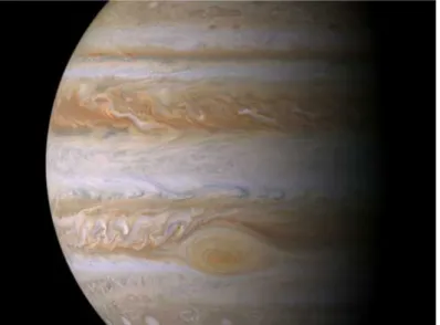
Jupiter is a striped huge spherical body without topography (Bagenal et al., 2004), whose atmosphere is the vastest in the solar system, governed by strong east-west winds (NASA, 2011). The horizontal bands are tra-ditionally divided into zones (white bands) and belts (dark bands) which rotate the opposite way. The winds generate giant long-lasting storms, the greatest is known as the Great Red Spot and spins near Jupiter’s equator. The clouds are made mostly of ammonia while water concentrations can be found at depth. The boundaries between atmosphere and deeper lay-ers are not well-defined, conventionally the atmosphere extends down to a pressure of 20 bar (Seiff et al., 1998). The planet is the fastest spinner of the solar system, its day lasting only 9.9 hours on average, in fact the rotation period is 5 minutes longer at the poles than at the equator, making Jupiter a differential rotator.
Figure 1.12:Jupiter with the visible Great Red Spot. Image credit: NASA.
change of state of the hydrogen, which becomes electrically conductive and behaves like a metal. Considering that Jupiter spins exceptionally fast, this phenomenon generates the impressive magnetic field, characteristic of the planet (NASA, 2011). Auroras take place on Jupiter, very similarly to what happens in some regions of the Earth, yet the phenomenon is much more powerful and amplified. Jupiter’s magnetic field traps great quantities of electrons and ions that are accelerated, creating immense electrics current and thus, the auroras (NASA, 2011).
The current knowledge of the interior structure of Jupiter envisages a radial division into three main layers (Bagenal et al., 2004). From top to bottom (Figure 1.13) these are:
- a helium-poor molecular hydrogen envelope which includes the at-mosphere;
- deeper, a helium-rich metallic hydrogen envelope; - a central dense liquid core of uncertain composition.
The upper atmosphere deficiency of helium can be explained by its separation into metallic hydrogen that takes place at depth, though this hypothesis requires the presence of a deeper helium-rich region. The two regions are homogeneous in composition thanks to convective phenomena and are separated by a narrow in-homogeneous region in which helium de-mixing occurs (Bagenal et al., 2004). The extent and position of this region remains a key question about the planet’s interior. The measure of Jupiter’s gravitational moments postulates the presence of a dense core, though its compositions and structure is still unknown (Bagenal et al., 2004).
The task of the new missions to Jupiter, regarding the interior of the planet, is to constrain three fundamental parameters:
- the mass of the core;
- the mass mixing ratio of heavy elements in the molecular region; - the mass mixing ratio of heavy elements in the metallic region.
For centuries Saturn has been, in the collective imagination, the only planet to possess rings. In truth, fainter rings formed also around Jupiter
Figure 1.13:View of Jupiter’s interior. Image credit: Burkhard Militzer at Univer-sity of California, Berkeley.
equatorial belt, consisting of thin dusts related to the formation of its biggest moons (NASA, 2011).
1.3.2 Ganymede
Ganymede is the largest natural satellite of the solar system with a mean radius of 2631.2 ± 1.7 km (Bagenal et al., 2004), is larger than Mer-cury and its size is about three quarters of that of Mars. This moons is the typical icy satellite composed of mostly water and silicates.
Early gravity measurements indicate a mean density for Ganymede of 1942.0 ± 4.8 kg/m3 (Bagenal et al., 2004), pointing to a partial differentia-tion of the satellite between the icy surface and the rocky core (McKinnon and Parmentier, 1986, Schubert et al., 1986). Moreover, the presence of a self-generated magnetic field suggests that the differentiation process has gone even further, leading to a three-layer model: water-ice shell, a rock mantle and a metallic core (Schubert et al., 1996). Crary and Bagenal (1998)
pointed out that, even rock cores that have high magnetic susceptibility (because rich in magnetite) cannot be sufficiently magnetized by the exter-nal Jovian field. Thus they indicate the metallic core as the possible and more plausible cause of Ganymede’s intrinsic magnetic field. Also, Schu-bert et al. (1986) concluded that the mentioned magnetic field is generated by dynamo action in a liquid or partially liquid metallic core. In both cases a metallic core for Ganymede is required.
Figure 1.14:View of the interior structure of Ganymede. Image credit: NASA.
The Galileo mission collected several pieces of evidence for a subsur-face ocean at Ganymede (Kivelson et al., 2002). The spacecraft detected an induced magnetic field at shallow depths (100-200 km underneath Ganymede’s surface) in response to the huge Jovian magnetosphere, usually associated to the presence of salty, conductive liquid water (Kivelson et al., 2002). However the interpretation of the magnetometer data proved quite chal-lenging, due to interference from Ganymede’s intrinsic magnetic field. Still, the evolution model of Ganymede based on its topography is compatible with a subsurface, salty, conductive ocean amidst two high-pressure ice layers. Nonetheless, its composition, location and extension are still un-known. A solid detection of a global ocean requires the measure of its tidal deformation, whose entity would be much larger in case of presence of liquid layers. Only gravitational measurements collected by a dedicated
space mission to Jupiter’s moon will confirm the existence of liquid water reservoirs, local or global, within Ganymede’s surface layer.
Ganymede possesses sufficient mass to attract and retain a thin atmo-sphere. The Hubble telescope has detected the presence of atomic oxygen by means of Far Ultra Violet (FUV) observations (λ = 130.4 - 135.6 nm). The atomic oxygen results from the dissociation of molecular oxygen, which is the dominant species of the atmosphere, due to incident collisions with free electrons. The column density of Ganymede’s atmosphere probably ranges between 1 ÷ 10 · 1014cm−2(Hall et al., 1998). In turn, the molecular oxygen might come from the dissociation of water molecules on Ganymede’s sur-face, as a result of incident radiation. The hydrogen is, on the other hand, scattered because of its small density.
1.3.3 Callisto
Callisto is the outermost of the Galilean moons, its mean radius is about 200 km smaller than Ganymede’s, and its density is very similar to that of the bigger moon, being 1834.4 ± 3.4 kg/m3(Bagenal et al., 2004).
Callisto formation occurred after Jupiter’s cooling, allowing the consol-idation of water masses into ice and preventing the vaporization of volatile elements. Callisto surface is ancient, dark, heavily cratered and, unlike Ganymede, shows no evidence for geological internal activity. This kind of information led to the conclusion that Callisto was undifferentiated (Schu-bert et al., 1981, 1986). However, gravity measurements from the Galileo mission indicated that Callisto interior was, at least partially, differentiated (Anderson et al., 1998, 2001). Even more surprisingly, magnetometer ob-servations detected signatures characteristic of an induced magnetic field, evidence for a subsurface ocean at Callisto (Zimmer et al., 2000). Despite the apparent lack of internal activity, the high-resolution camera onboard Galileo, revealed the presence of erosion and degradation processes on the surface of Callisto. These phenomena are caused by the exposition to the severe and highly-corrosive Jovian environment, giving Callisto the char-acteristic lumpy look.
Figure 1.15:View of the interior structure of Callisto. Image credit: NASA/JPL-Caltech.
A simple layered model has been proposed for Callisto, consisting of (Bagenal et al., 2004):
- a denser (more rock and dense-ice-phase rich) interior;
- a less rock-rich and more low-density ice-polymorph-rich shell; The depth at which the layers differentiate obviously depends on the mean densities. The upper limit of the interior density is that of a cool, undifferentiated and dehydrated rock+metal (3850 kg/m3). This condition would set the extension of the outer shell to 1250 km, while the lower limit is represented by the case of a clean-ice shell with or without a water ocean, for an extension of 300 km (Bagenal et al., 2004).
The existence of this two-layer model is legitimated by the fact that ice and rock can separate either by melting of the ice or by sinking of the rocks through ice. Considering the latter phenomenon, a rocky core could form, surrounded by a rock+ice layer and an outer shell, leading to a three-layer model (Mueller and McKinnon, 1988). In this model, the core of Callisto is composed of (18± 4) % of its total rock and extends up to 900 km in radius (Bagenal et al., 2004). The ocean would lay between the rock+ice layer and the pure ice shell, where thermal conditions leading to the melting of ice operate at the ice minimum-melting temperature.
1.3.4 Europa
The size of this satellite makes it the smallest among the Galilean satel-lites, despite that, Europa is, perhaps, the most interesting body in the Jo-vian system. Unfortunately the harsh radiation environment makes its ex-ploration very challenging. The estimated mean radius is 1565.0 ± 8.0 km, for a mean density of 2989 ± 46 kg/m3 (Bagenal et al., 2004).
Gravity measurements collected by the Galileo spacecraft show that the satellite is likely to be differentiated and a three-layer model has been proposed, consisting of (Anderson et al., 1997):
- a metallic core (mostly iron); - a silicate mantle;
- a water ice-liquid outer shell.
As always, gravity interpretations are not unique and there still is un-certainty on the state of the core and the outer shell, that could be either solid or fluid. For instance the interior could be composed of a mixture of silicates and metal, surrounded by an ice-water shell (Bagenal et al., 2004). For the latter, a mean density of 1050 kg/m3 is assumed, while for the core two different options exist (Bagenal et al., 2004):
a) a Fe core of density 8000 kg/m3, in this case the radius of the core could be only as large as 13% of Europa radius if the ice shell is 170 km thick;
b) a Fe-FeS core of density 5150 kg/m3, corresponding to a core radius as large as 45% of Europa radius, with 100 km thickness of ice. Given the uncertainty on the composition of the mantle, it is not possi-ble to set a lower bound on the radius of the core, however, the density of this mid layer must be at least 3800 kg/m3, implying that the mixture must be rich in metal and cannot be purely rock (Bagenal et al., 2004). Further-more, supposing the mantle density is at least 3000 kg/m3, the outer shell must be at least as thick as 80 km, in order to fulfill the constraint on the mean density.
Figure 1.16:View of the interior structure of Europa. Image credit: NASA/JPL-Caltech.
Galileo magnetometer observations have not detected an intrinsic mag-netic field at Europa (Schilling et al., 2004), thus they do not provide infor-mation about the state of the core (Bagenal et al., 2004). The generation of an internal magnetic field requires the core to be at least partially molten, however, the lack of dynamo action does not exclude a liquid core, in fact this could still be fluid but non convective (Bagenal et al., 2004).
Different conclusions can be drawn regarding the state of the outer shell, in fact observations have demonstrated that Europa responds to the time-variant magnetic field of Jupiter producing internal electric currents (Bagenal et al., 2004). In turn, these currents produce an induced magnetic field, providing information on the electrical conductivity, depth and thick-ness of the conductive region within Europa. Zimmer et al. (2000) located this region within 200 km of the surface, with an electrical conductivity compatible with that of sea water, postulating the presence of a subsurface ocean at Europa (see Figure 1.16).
1.4
Radio science experiments
Radio science experiments (RSE) exploit the radio-frequency link be-tween a spacecraft and ground stations, in order to determine crucial pa-rameters related to physical properties of a celestial body. In general, the
main scientific goals pursued by this kind of experiments can be summa-rized as:
- determination of a planetary gravity field; - study of a planetary surface;
- study of a planetary atmosphere.
In the frame of this work, this section will be dedicated to the imple-mentation of gravity experiments onboard recent missions to the Jupiter system. By means of radiometric observations, one can determine several parameters characterizing planetary gravity fields and providing informa-tion on the interior models and structures of celestial bodies. To this end, changes in phase, frequency and polarization of a microwave signal are analyzed and interpreted.
The success of gravity experiments strongly depends on technical char-acteristics of the onboard and ground equipment, but also on optimal mis-sion conditions. In the following subsections, a detailed description of the instruments composing the radio science system will be provided.
1.4.1 Space segment
The key onboard instrument of a state-of-the-art radio science experi-ment is the Ka-band transponder, which is able to establish radio links with ground characterized by high phase stability. The crucial innovative aspect of the newest experiments is the exploitation of the Ka-band of the electro-magnetic spectrum (26.5 - 40.0 GHz), both in up-link and down-link. The transponder can also operate in a multi-frequency configuration (with X-band links, 7.0 to 11.2 GHz), so as to make possible the total cancellation of plasma noise in critical conditions, such as solar conjunctions (see Section 3.3.2).
In the triple-link configuration, two uplink and three downlink carrier signals are employed at the same time:
- X-band (8.4 GHz) downlink and X-band (7.2 GHz) uplink; - Ka-band (32.5 GHz) downlink and X-band (7.2 GHz) uplink;
Figure 1.17:Triple-link configuration of the Ka-band transponder (ESA, 2011).
- Ka-band (32.5 GHz) downlink and Ka-band (34.0 GHz) uplink.
The main link used for gravity science investigation is the Ka-Ka link. Radiometric measurements are characterized by high accuracies, in partic-ular range-rate measurements (radial velocity of the spacecraft) can be as well resolved as 3µm/s @ 1000 s integration time, while the average accu-racy of a range measurement (radial distance of the spacecraft) is about 20 cm for a two-way link.
All measurements must be carried out in a coherent way, using fre-quency standard characterized by high stability (hydrogen masers) for the generation and conversion of the carrier. The Ka-band transponder sup-ports an innovative wide-band Pseudo Noise (PN) ranging modulation scheme for the carriers (Thales, 2012).
A very important parameter characterizing the Ka-band transponder is the phase stability and the group delay, which is, currently, better than 0.1 ns pk-pk over a time of 36 hours (Thales, 2012). Aging effects on the KaT could degrade the group delay stability, jeopardizing the accuracies on range measurement. The KaT Allan deviation is also indicative of the frequency stability of the instrument. At this stage of development, the Allan deviation is assured to be better than 10−15.
For further information, the technical performance of the KaT can be found in Table 1.4, where information about the mass and power consump-tion are reported as well (Thales, 2012).
Figure 1.18:The Ka-band transponder (Thales, 2012). Image credit: Thales Alenia Space.
Mass 3 kg
Power consumption <40 W (for 32 dBm output power)
Dimension (LxWxH) 215x140x175 mm
Qualification temperature range 20/+65◦C (operative)
Design life >15 Years
Acquisition threshold -131 dBm @ 4 kHz/s Tracking threshold -135 dBm @ 1.2kHz/s (-138 dBm @ 400 Hz/s) Turn-around ratio 3360/3599 Output power Up to 35 dBm @ 32GHz Allan Deviation ≤4x10⁻¹⁶ @ 1000s Doppler shift ±6 MHz Noise figure <4 dB
PN Ranging Chip rate up to 25 Mcps
Transparent Ranging BW 27 MHz
Mixed Ranging low-frequency BW 4 MHz
KaT Group-delay stability ¡0.1ns pk-pk