Universit`
a della Calabria
Dipartimento di Matematica
Dottorato di Ricerca in Matematica ed Informatica
xxiii ciclo
Settore Disciplinare MAT/05 – ANALISI MATEMATICA
Tesi di Dottorato
Convex Tomography
in dimension two and three
Marina Dicosta
Supervisore
Coordinatore
Prof. Aljoˇsa Volˇciˇc
Prof. Nicola Leone
Abstract
In this thesis we investigate a problem which is part of Geometric Tomography. Geometric Tomography is a branch of Mathematics which deals with the determi-nation of a convex body (or other geometric objects) in n from the measure of its
sections, projections, or both. In particular, it is focused on finding conditions suffi-cient to establish the minimum number of point X-rays needed to determine uniquely a convex body in n.
The interest for this particular mathematical subject has its roots in the studies re-lated to Tomography.
Nowadays it is rare that someone has never heard of CAT scan (Computed Assisted Tomography). This medical diagnostic technique, born in the late 70s, allows us to reconstruct the image of a three-dimensional object by a large number of projections at different directions. It is useful to emphasize that CAT is a direct application of a pure mathematical instrument known as ‘the Radon transform”.
From the mathematical point of view, the question of when a convex body, a compact convex set with nonempty interior, can be reconstructed by means of its X-ray, arose from problems (published in 1963) posed by Hammer in 1961 during a Symposium on convexity:
« Suppose there is a convex hole in an otherwise homogeneous solid and that X-ray pictures taken are so sharp that the “darkness” at each point determines the length of a chord along an X-ray line. (No diffusion please). How many pictures must be taken to permit exact reconstruction of the body if:
(a) The X-rays issue from a finite point source? (b) The X-rays are assumed parallel? »
A convex body is a convex compact set with nonempty interior.
We distinguish between two problems, according to the X-rays are at a finite point i
ii source or at infinity.
We are searching which properties a set of directions U must fulfill, in order to deter-mine uniquely a convex body K by means of its (either parallel or point) X-rays, in the directions of U. When U is an infinite set then this reconstruction is possible and this follows from general theorems regarding the inversion of the Radon transform. This thesis consists of two parts. The first (Chapter 3) is concerned with the deter-mination of a planar convex body from its i-chord functions, while the second part (Chapter 4) generalizes the planar results to the three-dimensional case. The main results provide a partial answer to the problem posed by R. J. Gardner:
“How many point X-rays are needed to determine a convex body in n?”
We use two analytic tools both considered in geometric tomography for the first time by K. J. Falconer. One is the i-chord function, which is related through the Funk theorem to the measures of the i-dimensional sections, when i is a positive integer. The other tool, inspired by a paper by D. C. Solmon, suggested the introduction of a kind of “Cavalieri Principle” for point X-rays, and has been later on extended to other dimensions and real values of i.
The i-chord functions allow to translate in analytical form the information given by the ith section functions. Therefore, from an analytical point of view we have the following problem:
“Suppose that K ⊂ nis a convex body and let p
h be some noncollinear
points (some of them are possibly at infinity). Suppose, moreover, that we are given the i-chord functions at the points ph, with i ∈ . Is K then
uniquely determined among all convex bodies?”
The i-chord functions ρi,K can be seen as a generalization of the radial function of
the convex body K. The latter is the function that gives the signed distance from the origin to the boundary of K. For integer values of the parameter i, the i-chord function is closely linked to the ith section function of a convex body, that is the function assigning to each subspace of dimension i the i-dimensional measure. When i = 1, the 1st section function coincides with the 1-chord function, that is the point X-ray of the convex body at the origin.
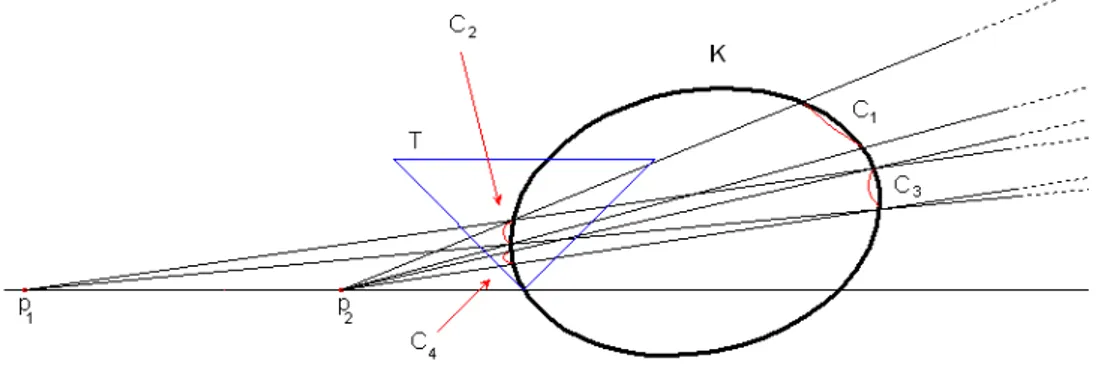
In Chapter 3 we consider two planar problems. One problem consists of the deter-mination of a planar convex body K from the i-chord functions, for i > 0, at two points when the line l passing through p1 and p2 meets the interior of K and the two
points p1 and p2 are both exterior or interior to K. If the line l supports K, then
iii convex body K from its i-chord functions at three noncollinear points for 0 < i < 2. Chapter 4 deals with the problem of determining a three-dimensional convex body K from the i-chord functions at three noncollinear points non belonging to K. Also in this case we search a sort of “Cavalieri Principle”, for a suitable measure involving i-chord functions for 1 < i < 3.
We are not able to extend this result to generic convex bodies when i = 1. In this case we have to assume that the convex body is of class C1+α with α ∈]0, 1[.
Sommario
Il lavoro di tesi si inserisce prevalentemente nell’ambito della ricostruzione delle immagini, in particolare nel settore della Tomografia Geometrica, la quale si occupa di trovare il minor numero di radiografie necessarie per ricostruire univocamente un corpo. La teoria generale, basata sul concetto di Trasformata di Radon trova una sua significativa applicazione in medicina nella Tomografia Computerizzata, che consente la ricostruzione dell’immagine di una sezione del corpo umano mediante l’uso dei raggi X presi in diverse direzioni. Dal punto di vista matematico, il problema di quando un corpo convesso (o un altro oggetto geometrico), può essere ricostruito per mezzo delle sue radiografie, si è sviluppato grazie ai problemi posti nel 1961 da P.C. Hammer all’American Mathematical Society Symposium sulla Convessità:
“Suppose there is a convex hole in an otherwise homogeneous solid and that X-ray pictures taken are so sharp that the “darkness” at each point determines the length of a chord along an X-ray line. (No diffusion please). How many pictures must be taken to permit exact reconstruction of the body if:
(a) The X-rays issue from a finite point source? (b) The X-rays are assumed parallel?”
Un corpo convesso è un insieme convesso compatto dotato di punti interni. Ci si trova dunque di fronte due problemi, a seconda che le radiografie siano prese da sorgenti finite, o all’infinito. Ci chiediamo allora quali proprietà deve soddisfare un insieme di direzioni U, affinché un corpo convesso K sia univocamente determinato dalle sue radiografie (parallele o puntuali) nelle direzioni in U. Nel caso in cui U è un insieme infinito questo è vero e sussistono dei teoremi di unicità basati sull’inversione della Trasformata di Radon. Il lavoro di tesi è suddiviso fondamentalmente in due parti. Una prima parte (Capitolo 3) si occupa dello studio della determinazione di un corpo convesso planare per mezzo delle funzioni i-cordali, mentre la seconda
v parte (Capitolo 4) generalizza quanto visto nel caso planare, al caso tridimensionale. I risultati ottenuti forniscono una parziale risposta al problema posto da R. J. Gardner:
“How many point X-rays are needed to determine a convex body in n?”
Vengono utilizzati due strumenti analitici, entrambi introdotti per la prima volta da K. J. Falconer nell’ambito della tomografia geometrica. Il primo è la funzione i-cordale, la quale è legata per mezzo del Teorema di Funk alle misura della sezione i-dimensionale, quando i è un numero intero positivo. Il secondo strumento, ispirato da un articolo di D. C. Solmon, è stato la ricerca di una opportuna misura che fornisse una specie di “Principio di Cavalieri” per le funzioni i-cordali.
Le funzioni i-cordali costituiscono uno strumento essenziale che permette di tradurre in forma analitica le informazioni date dalle funzioni di i-sezione. Pertanto, dal punto di vista analitico si ha il seguente problema:
“Supponiamo che K ⊂ n sia un corpo convesso e siano p
h dei punti non
allineati (alcuni dei quali eventualmente all’infinito). Supponiamo inoltre di conoscere le funzioni i-cordali in ph per i ∈ . K è univocamente
determinato tra tutti i corpi convessi?”
Le funzioni i-cordali ρi,K possono essere viste come una generalizzazione della
fun-zione radiale del corpo convesso K. Quest’ultima è la funfun-zione che fornisce la distanza con segno dall’origine al bordo di K. Per valori interi del parametro i, le funzioni i-cordali sono strettamente collegate alle funzioni i-sezione di un corpo convesso, ovvero la funzione che fornisce la misura i-dimensionale dell’intersezione con un sottospazio avente dimensione i. Quando i = 1, la funzione 1-sezione coincide con la funzione 1-cordale, ovvero con la radiografia puntuale nell’origine.
Nel Capitolo 3 affrontiamo due problemi planari. Uno consiste nella determinazione di un corpo convesso K prendendo le funzioni i-cordali, per i > 0, in due punti nel caso in cui la retta l passante per p1 e p2 interseca la parte interna di K e i punti
sono entrambi esterni o interni a K. Se la retta l supporta K, i risultati ottenuti valgono solo per i ≥ 1. Il secondo risultato riguarda la determinazione di un corpo convesso planare K dalle funzioni i-cordali in tre punti non allineati per 0 < i < 2. Nel Capitolo 4 affrontiamo il problema di determinare un corpo convesso tridimen-sionale K prendendo le funzioni i-cordali per tre punti non allineati ed esterni a K. Anche in questo caso si cerca una specie di “Principio di Cavalieri” per un’opportuna misura che coinvolga le funzioni i-cordali in tre punti non allineati per 1 < i < 3. Non è stato possibile estendere questo risultato a corpi convessi generici per i = 1. In questo caso si deve richiede che il corpo convesso sia di classe C1+α con α ∈]0, 1[.
Contents
1 Preliminary Topics 8
1.1 Notations and definitions . . . 8
1.2 Integral transforms . . . 10
1.3 X-ray transforms . . . 12
1.4 Basic notions on differentiability . . . 16
Introduction 8 2 The i-chord functions 19 2.1 Radial function and i-chord function . . . 19
2.2 The ith section function . . . 24
2.3 i-chord function and ith section function . . . 25
2.4 The corresponding components . . . 28
3 Determination of planar convex bodies by i-chord functions 35 3.1 i-chord functions of planar convex bodies . . . 35
3.2 A two-point solution . . . 47
3.3 A three-point solution . . . 67
4 Three-dimensional case 73 4.1 The measure µk and its properties . . . 74
4.2 The Groove . . . 78
4.3 Uniqueness results . . . 81
5 Conclusions and open problems 93
Bibliography 97
Introduction
“Stay hungry, stay foolish.” Steve Jobs, 5th June 2005
In this thesis we will investigate a problem which belongs to Geometric Tomog-raphy. Geometric Tomography is a branch of Mathematics which deals with the determination of a convex body in n from the measure of its sections, projections,
or both. In particular, it is focused on finding conditions sufficient to establish the minimum number of point X-rays needed to determine uniquely a convex body in
n.
The interest for this particular mathematical subject has its roots in the studies related to Tomography. The word “tomography” is derived from the Greek τ ´oµoς (tómos –slice) and γρ´αϕ'ιν (gráphein – to write).
Nowadays it is rare that someone has never heard of CAT scan (Computed Assisted Tomography). This medical diagnostic technique, born in the late 70s, allows us to reconstruct the image of a three-dimensional object by a large number of projections in different directions. The first CT-scanner, was conceived for EMI in 1967 by Sir Godfrey Newbold Hounsfield, an English electrical engineer at Atkinson Morley Hos-pital in Wimbledon, London. This device, called “EMI-scanner” was the first able to display cross-sections of the human body, particularly of the skull (1 October 1971). Though extremely innovative, this tomograph took many hours to get data, and sev-eral days for producing the images. This marks the beginning of a new frontier of medicine just called Computed Tomography, in fact, the term “computed tomogra-phy” refers to the computation of tomography from X-ray pictures.
A few years later, in 1979 Hounsfield along with Allan McLeod Cormack, a South African-born American physicist, were awarded the Nobel Prize in Medicine.
Later improvements have been possible thanks to the increased power of computers, a better technology in data collection and better reconstruction algorithms.
After this brief introduction, it is useful to emphasize that CAT is a direct application 1
INTRODUCTION 2
of a pure mathematical instrument known as “the Radon transform”, named after the Austrian mathematician who in 1917 introduced this kind of transform during his research in measure theory.
In 1917 Johann Radon published his paper, Über die Bestimmung von Funktionen durch ihre Integralwerte längs gewisser Mannigfaltigkeiten, (to which little attention was paid for a long time) with which Radon can be recognized as the father of to-mography. Radon did not mean his transform to be used for a medical application. We will give next a brief description of the process implemented in the CAT, as well as its existing relationship with the Radon transform.
To perform a radiography, the patient is placed between a X-ray generator and a film sensitive to X-rays or a digital detector. According to the density and composition of the different areas of the object a proportion of X-rays are absorbed by the object. The X-rays that pass through are then captured behind the object by the detector, which gives a two-dimensional representation of all the structures superimposed on each other.
From the mathematical point of view, the question of when a convex body, a compact convex set with nonempty interior, can be reconstructed by means of its X-ray, arose from problems posed by Hammer in 1961 during a Symposium on convexity, [24].
« Suppose there is a convex hole in an otherwise homogeneous solid and that X-ray pictures taken are so sharp that the “darkness” at each point determines the length of a chord along an X-ray line. (No diffusion please). How many pictures must be taken to permit exact reconstruction of the body if:
(a) The X-rays issue from a finite point source? (b) The X-rays are assumed parallel? »
It is rather surprising how clear was Hammer’s idea on the reconstruction of objects from X-rays so many years before anybody figured out to use the Radon transform for CT-scanners.
We distinguish between two problems, according to the X-rays are at a finite point source or at infinity.
We are now searching which properties a set of directions U must fulfill, in order to determine a convex body K in a unique way by means of its (either parallel or point) X-rays, at the directions of U. When U is an infinite set then this reconstruction is possible and there are a lot of uniqueness theorems based on the inversion of the Radon transform, [23] and [42]. In particular Zalcman, [50, Section 2], states that
INTRODUCTION 3
K is uniquely determined if the lengths of the chords are given from infinitely many directions.
State of art
The problems considered in our thesis are of a different nature and are probably of less practical application.
There are several paper in the literature which study the reconstruction of a convex body in n, for n ≥ 2, from the measures of their intersections with affine subspaces
of dimension k, with 1 ≤ k ≤ n − 1. There is a first group of papers that gives conditions on the position and number of points p1, p2, . . . , pm (some possibly at
infinity) which guarantee the uniquely determination of a convex body K in nby the
measures of the intersections of K with all the affine subspaces, of a given dimension k, passing through ph, for 1 ≤ h ≤ m. For example, [17], [11], [9], [10], [44], [14],
[13], [18], [39], [44], [46] and [20].
A second group of papers, on the other hand, fixes a point p and ensure that K is uniquely determined by the measures of the intersections of K with the affine subspaces through p of (at least) two different dimensions, [18] and [49]. The earliest papers concern Hammer’s question (b). The (parallel) X-ray of a convex body K in the direction u is the function giving the lengths of all the chords of K parallel to u. The uniqueness aspect of question (b) is equivalent to asking which finite sets of directions are such that the corresponding X-rays distinguish between different convex bodies. Simple examples showed that there are arbitrarily large finite sets of directions that do not have this desirable property and that no set of three directions does it. In fact, three directions never suffices, since each triangle is affinely equivalent to an equilateral triangle, and, by a rotation of π
3 about the barycentre we can build a
different equilateral triangle with equal X-rays along the three directions connecting the corresponding vertices.
The first studies were made, independently, by Falconer [11] and Gardner [13]. A complete solution was found by Gardner and McMullen, [17], (see also [16, Chapter 1]). A corollary of their result is that there are sets of four directions in S1, the
unit disk in 2 such that the X-rays of any planar convex body in these directions
determine it uniquely among all planar convex bodies. It also was shown in [17] that a suitable set of four directions is one such that the corresponding set of slopes has a transcendental cross-ratio. Clearly this is an impractical choice of directions.
INTRODUCTION 4
However, Gardner and Gritzmann, [19] showed that further suitable sets of four directions are those whose set of slopes, in increasing order, have a rational cross-ratio not equal to 3
2, 43, 2, 3, or 4.
The corresponding uniqueness problem in higher dimensions can be solved by taking four directions, as specified above, all lying in the same two-dimensional plane. Since the corresponding X-rays determine each two-dimensional section of a convex body parallel to this plane, they determine the whole body.
The point X-ray of a convex body K at a point p is the function giving the lengths of all the chords of K lying on lines through p.
The position of the sources with respect to the convex body is important.
Parallel X-rays can be viewed as a limit case of point X-rays, where the sources lay on the line at infinity, namely the set of points at infinity of each line in the plane. It is easy to see that a single source p does not suffice. The only known result in the opposite direction is provided by a paper of Lam and Solmon [28] which proves that, with some exceptions, convex polygons are uniquely determined among convex polygons by one point X-ray. In fact, they in [28] show an algorithm for the reconstruction of a convex polygon from one directed X-ray at the origin.
One of the problems is that Cavalieri’s principle does not hold for point X-rays, since the area increases for increasing distance from the sources. Consequently, new measures has been introduced,for which a kind of Cavalieri principle holds.
The uniqueness aspect of Hammer’s question (a) is not completely solved, but it is known that a planar convex body K is determined uniquely among all planar convex bodies by its X-rays taken at
(i) two points such that the line through them intersects K and it is known whether or not K lies between the two points. (see Falconer, [9] and [11] and Gardner, [16, Theorem 5.3.3]);
(ii) three points such that K lies in the triangle having these three points as vertices. (see Gardner [16, Theorem 5.3.6]);
(iii) any set of four collinear points whose cross ratio is restricted as in the parallel X-ray case above. (see Gardner, [14]);
(iv) any set of four points in general position. (see Volčič, [44]).
Except in the case of (i), little is known about the uniqueness problem for point X-rays in higher dimensions. Many of these results have been extended to spaces of constant curvature. For example, Dulio and Peri in [2] and in [3] establish a version
INTRODUCTION 5
of [16, Theorem 5.3.3]) that holds in spaces of constant curvature. In particular, in [4], they show that convex bodies in a plane of constant curvature are determined (up to reflection in the origin, in the case of the sphere) by point X-rays at four points in general position. The main result in [17] (see also [16, Theorem 1.2.11]) is that a planar convex body is determined, among all planar convex bodies, by its parallel X-rays in a finite set U of directions if and only if U is not a subset of the directions of edges of an affinely regular polygon. This gives many choices for sets U with the uniqueness property. For example, Gardner and Gritzmann, [19] showed that U can be any set of at least seven directions with rational slopes, but as mentioned above, the minimum number of directions in U is four.
Most of the existing literature provide uniqueness theorems and does not address the problem of actual reconstruction. Only recently a paper of Gardner and Kiderlen, in [20], proposed algorithms for reconstructing a planar convex body K from either its parallel X-rays taken in a fixed finite set of directions or its point X-rays taken at a fixed finite set of points. The two algorithms construct a convex polygon Pk
whose X-rays approximate (in the least squares sense) k equally spaced noisy X-ray measurements in each of the directions or at each of the points. Pk, almost surely,
tends to K in the Hausdorff metric as k tends to infinity. This result provides a solution, in the strongest sense, of the Hammer’s X-ray problems.
Hammer actually asked his questions in 1961, a year before (independently) the re-sults obtained by Giering. In [21], he studied one of these problems proving that given a planar convex body K chord lengths in three appropriate directions (de-pending on K) are enough to distinguish from any other planar convex body the Steiner Symmetrals of K about lines in those directions. Volčič in [46] provides a new proof of this result, and permits a wider choice of triplets of directions, possi-bly also on a finite line, and also Gardner in [13] gives a shorty version of Giering’s result. Furthermore, Giering has shown that two directions are in general not enough. Zuccheri in [51] describes a method for computing jth derivatives of the polar representations of the boundary of a convex body K, from generalized i-chord func-tions at two points not lying on the boundary of K, ∂K, but such that the line l passing through these two points meets ∂K at two distinct points. On the other hand, Falconer in [11] and in [9] provides methods for computing these intersection points for i-chord functions for i ∈ . L. Zuccheri extends these methods to the val-ues of i < 1, and observes that these intersection points can be obtained by solving
INTRODUCTION 6
a system of algebraic equations.
Main results
The aim of this thesis is to extend to the case of i-chord functions the main results obtained for i = 1 by Volčič in [44] and by Gardner in [16].
The notion of i-chord functions has been introduced by Falconer in [11] for integer values 0 < i < n, where n is the dimension of the Euclidean space n in which the
problem is handled.
The i-chord functions ρi,K are generalizations of the radial function of the convex
body K. The latter is the function that gives the signed distance from the origin to the boundary of K. The i-chord functions are particularly useful when i is an integer strictly between 0 and n, but other values are also relevant, as in the various forms of the notorious equichordal problem. The i-chord functions has been extended to all integer values by Gardner in [14] and to all real numbers in [16].
For integer values of i, the i-chord function is closely related (via Funk theorem) to the ith section function of a convex body, the function giving the i-dimensional volumes of its intersections with i-dimensional subspaces.
When i = 1, the ith section function coincides with the 1-chord function, also known as the point X-ray at the origin (or, in the computer tomography, the fan-beam X-ray at the origin). The (n − 1)th section function is simply called the section function. The i-chord function is a technical tool which allows to translate in analytical form the information given by the ith section function. Therefore, from an analytical point of view we have the following problem:
« Suppose that K ⊂ n is a convex body and let p
h be some noncollinear
points (some of them are possibly at infinity). Suppose, moreover, that we are given the i-chord functions at the points ph, with i ∈ . Is K then
uniquely determined among all convex bodies? »
A second tool used throughout this thesis is a kind of “Cavalieri Principle” for a measure νi having an appropriate invariance property involving the i-chord
func-tions. The Cavalieri principle, introduced for i = 1 in [44] and for all integers in [14], can be in fact extended to all real values as shown in [16].
The main contribution of the work reported in this thesis are summarized in the following.
INTRODUCTION 7
First of all, we will show the determination of a planar convex body K from the i-chord functions, for i > 0, at two points when the line l passing through p1 and p2
meets the interior of K and the two points p1 and p2 are both exterior or interior
to K, and it is known where K meets the line l. If the line l supports K, then the results will hold for i ≥ 1.
A second relevant result will concern the determination of a planar convex body K from its i-chord functions at three noncollinear points for 0 ≤ i < 2. In particular, when the convex body is contained in the interior of the triangle formed by the three points the result will hold for i > 0.
Finally we will tackle the problem of determining a three-dimensional convex body K from the i-chord functions at three noncollinear points non belonging to K using a sort of “Cavalieri Principle”, for a suitable measure involving i-chord functions for 1 < i < 3.
Moreover we will give an uniqueness result for convex bodies of class C1+α with
α ∈]0, 1].
Outline of this thesis
The thesis is organised as follows.
First, basic notations and definitions on convexity are introduced in Chapter 1, more-over, integral transforms and X-ray transform are also discussed and basic notions on differentiability are provided.
Then, a wider presentation of the notion of i-chord function is introduced in Chapter 2, where its relationship with the concepts of ith section function and of X-ray of order i is also discussed. In particular, the important tool of the corresponding components is provided.
After that, the determination of a planar convex body from its i-chord functions is discussed in Chapter 3.
Afterwards, uniqueness results regarding the three-dimensional case are presented in Chapter 4.
Chapter 1
Preliminary Topics
This chapter aims at introducing the main topics this thesis is about, giving concepts necessary to better understand the following chapters.
In particular, we will give concepts regarding convexity, integral transforms and their equivalent X-ray transforms, and finally we will recall some basics on differentiability. References for this material are [16], [32], [5, 6, 7], [33, 25], [23, 37, 26] and [36].
1.1
Notations and definitions
Let us now introduce some basic definitions and notations.
We denote the n-dimensional Euclidean space by n with the origin o.
Definition 1.1.1 (Convex set).
A set C in n is called convex if the line segment joining any pair of points of C lies
entirely in C.
Definition 1.1.2 (Convex body).
A convex body in n is a compact convex set with nonempty interior.
We denote by Kn the class of nonempty compact convex subsets of n, and by
Kn
0 the class of convex bodies.
We write int K and ∂K, respectively, for the interior and the boundary of K. We use the symbol K − p to denote the translated convex body:
K − p = {x − p : x ∈ K} .
We denote by G (n, k) the set of all k-dimensional linear subspaces of n, while by
G(n, k, u) we denote the set of all k-dimensional affine subspaces of nparallel to the 8
1.1 Notations and definitions 9
vector u belonging to the unit sphere Sn−1. With λ
k we denote the k-dimensional
Lebesgue measure. We employ the symbol lu for the line passing through o and
parallel to u ∈ Sn−1. For any A ⊂ n, we use the symbols lin A and aff A to
denote, respectively, the smallest linear subspace containing A and the smallest affine subspace containing A. Moreover, for every x ∈ n! {o}, and for every A ⊂ n, we
define pos x := {λx : λ ≥ 0} and pos A := conv ! x∈A {pos x : A ∩ pos x '= ∅} . We write pospA := p + pos (A − p)
for the convex positive half-cone with vertex p generated by A. Let E1, E2 ⊂ n
such that pospE1 = pospE2. Let l be any half-line issuing from p and intersecting
E1 (and so also E2). We say that E1 is between p and E2 if for any point x1 ∈ E1∩ l
and any x2 ∈ E2∩ l, x1 is between p and x2.
A simplex with vertices a1, a2, · · · , ak will be denoted by )(a1, a2, · · · , ak). Hence,
a simplex )(a1, a2) is the segment [a1; a2] with endpoints a1 and a2, while a simplex
)(a1, a2, a3) is the triangle with vertices a1, a2 and a3.
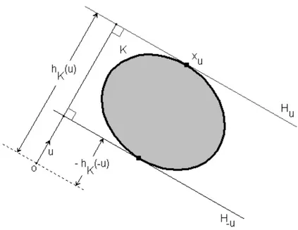
Definition 1.1.3 (Support function, supporting hyperplane). Let K ∈ Kn, the support function h
K of K is defined by
hK(x) = max {x · y : y ∈ K} ,
for x ∈ n.
If u ∈ Sn−1, the supporting hyperplane to K with outer normal vector is defined by
Hu = {x : x · u = hK(u)} .
The support function hK(u) at a unit vector u gives the signed distance from the
origin o to the supporting hyperplane Hu, (see Figure 1.1).
Since if K and K# are two nonempty compact convex sets, K ⊂ K# if and only if
hK ≤ hK!, it follows that a compact convex set is uniquely determined by its support
1.2 Integral transforms 10
Figure 1.1: The support function Definition 1.1.4 (Star-shaped set).
Let L ⊂ n and p ∈ n. The set L is star-shaped at a point p if its intersection with
every line through p is either empty or connected.
1.2
Integral transforms
Although the integral transforms can be defined more generally, it is assumed throughout this section that f ∈ L1
0(Ω), i.e., that f is integrable and vanishes outside
Ω, where Ω is a bounded open subset of n.
Definition 1.2.1 (Directed X-ray of f at a point p).
Let p ∈ n. The divergent beam transform, or directed X-ray, of f at the point p is
defined for each u ∈ Sn−1 by
Dpf (u) =
" +∞
0
f (p + tu)dt.
Physically the function f is the X-ray attenuation coefficient, i.e., the density of the object X-rayed, the point p is the X-ray source and the unit vector u is an X-ray detector. Therefore Dpf (u) represents the attenuation in the X-ray beam, i.e., the
1.2 Integral transforms 11
total mass of the object along the half-line issuing from p and having direction u. The role of computed tomography is to reconstruct this function f from a number of X-rays. The word tomography refers to the two-dimensional problem of the recon-struction of the cross sections of f . Historically, computed tomography began with parallel beam X-rays in which the photons travel along lines with a fixed direction rather than along rays emanating from a fixed point source.
Definition 1.2.2 (Parallel X-ray of f in the direction u).
Let u ∈ Sn−1. The X-ray transform, or parallel X-ray, of f in direction u is defined
for each x ∈ u⊥ and t ∈ by
Xuf (x) =
" +∞
−∞
f (x + tu)dt where dt denotes integration with respect to λ1.
Definition 1.2.3 (Radon transform).
The Radon transform of f is defined for t ∈ and u ∈ Sn−1 by
˜
f (t, u) = "
u⊥+tu
f (x)dx.
For each u ∈ Sn−1, Fubini’s theorem guarantees that ˜f (t, u) exists for almost all t.
Moreover, by the orthogonal decomposition theorem, the set H = u⊥+ tu represents
a hyperplane in n, therefore the Radon transform can be rewritten in the following
way ˜ f (H) = " H f (x)dx
so it is a function defined on the space of hyperplanes. The invertibility of the Radon transform makes possible bodies to be reconstructed completely, if all their X-ray pictures are given.
Definition 1.2.4 (X-ray of f at a point p).
Let p ∈ n. The line transform, or X-ray, of f at the point p is given by
Xpf (u) =
" +∞
−∞
f (p + tu)dt.
Observe that, the X-ray of f at the point p is linked to the directed X-ray of f in the directions u and −u by the following relation
1.3 X-ray transforms 12
for each u ∈ Sn−1, [36].
Definition 1.2.5 (k-dimensional X-ray).
Let 1 ≤ k ≤ n − 1 and S ∈ G (n, k). The k-dimensional X-ray, or k-plane transform, of f parallel to the subspace S is defined for each y ∈ S⊥ by
XSf (y) =
"
S
f (x + y)dx. Definition 1.2.6 (X-ray of order i).
Let p ∈ n and i ∈ . The X-ray of order i of f at p is defined for each u ∈ Sn−1 by
Xi,pf (u) =
" +∞
−∞
f (p + tu)|t|i−1dt.
The most interesting aspects of computed tomography are the questions of unique-ness and stability. Regarding uniqueunique-ness we have the following theorems proved in [16, 26, 37], and [23].
Theorem 1.2.7.
Let Ω be a bounded open subset of n and let f ∈ L1
0(Ω). Suppose that D ⊂ Sn−1 is
an infinite set. If Xuf = 0 for all u ∈ D, then f = 0, λn-almost everywhere.
Theorem 1.2.8.
Let Ω be a bounded open subset of the unit ball B in n and let f ∈ L1
0(Ω). Suppose
that P ⊂ n! B is an infinite set. If D
pf = 0 for all p ∈ P , then f = 0, λn-almost
everywhere.
These two uniqueness theorems for the divergent beams and line transforms, 1.2.7 and 1.2.8, state that any object, even with varying density, is uniquely determined by an infinite set of point X-rays. On the other hand, no finite set of point X-rays suffice.
1.3
X-ray transforms
For characteristic functions of bounded measurable sets the integral transforms, defined in the previous section, boil down to the following functions.
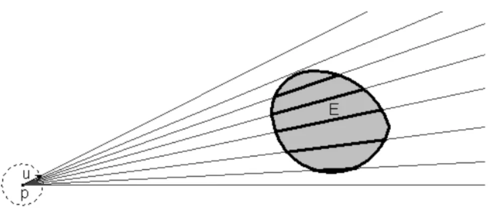
Definition 1.3.1 (Directed X-ray).
1.3 X-ray transforms 13
E at p is defined for λn−1−almost all u ∈ Sn−1 by
DpE(u) = Dp E(u) = λ1(E ∩ (ru+ p)),
where ru is the ray emanating through o parallel to u.
Figure 1.2: The directed X-ray of E at p
This function gives us information about the “lengths” of all the intersections of the set E with all the half-lines issuing from p, (see Figure 1.2).
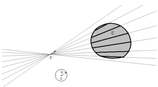
Definition 1.3.2 (X-ray).
Let p be a point and let E be a bounded measurable set in n. The X-ray of E at p
is defined for λn−1−almost all u ∈ Sn−1 by
XpE(u) = Xp E(u) = λ1(E ∩ (lu+ p)).
This function provides us the lengths of all the intersections of the set E with all the lines through p, (see Figure 1.3).
When E is a Borel set, Dp(E) and Xp(E) are defined everywhere on Sn−1. With
X-ray, we consider the rays issuing from p in both the directions u and −u as a single beam. For this reason, X-rays do not exist in nature but are merely a mathematical idealization.
The X-ray gives us less information than directed X-ray. For example, Figure 1.4 shows that two congruent disks have the same X-rays at the middle point of the
1.3 X-ray transforms 14
Figure 1.3: The X-ray of E at p
1.3 X-ray transforms 15
segment joining their centers, but they have different directed X-rays. In general
XpE(u) = XpE(−u)
for each u ∈ Sn−1, i.e., X
p(E) is even, while Dp(E) is not necessarily an even
function.
If E is a body star-shaped at p, each ray issuing from p meets E in a (possibly degenerate) segment, so the directed X-rays give the length of each line segment, while the X-rays give the length of the “two” line segments.
Definition 1.3.3 (X-ray of order i).
Let i ∈ . Let p be a point and E a bounded measurable set in n. The X-ray of
order i of E at p is defined by Xi,pE(u) =
" ∞
−∞
E(p + tu)|t|i−1dt,
for u ∈ Sn−1 for which the integral exists.
Note that when i = 1 we retrieve the definition of the X-ray of K at p. Definition 1.3.4 (k-plane transform).
Let ≤ k ≤ n − 1 and S ∈ G (n, k). The k-plane transform, or the X-ray, of f parallel to the subspace S is defined for each y ∈ S⊥ by
XSf (y) =
"
S
f (x + y)dx. Definition 1.3.5 (k-dimensional X-ray).
Let p be a point and let E be a bounded λn−measurable set in n. If 1 ≤ k ≤ n − 1,
we define the k-dimensional X-ray of E at p as a function on G (n, k) such that to each G ∈ G (n, k) assigns the measure λk(E ∩ (G + p)).
The X-ray of a convex body is related to the notion of Steiner symmetral, intro-duces by Jacob Steiner [41].
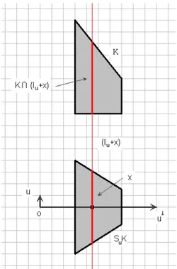
Definition 1.3.6 (Steiner symmetral).
Let K be a convex body in n. Let u ∈ Sn−1 and let l
u be the line through the origin
and parallel to u. For each x ∈ u⊥, let c(x) be defined as follows. If K ∩ (l
u+ x) is
empty, let c(x) = ∅. Otherwise, let c(x) be the segment on lu+ x centered at x whose
1.4 Basic notions on differentiability 16
Steiner symmetral of K and it is denoted by SuK. The mapping Su from Kn into
itself is called Steiner Symmetrization.
Notice that SuK has the same X-rays as K in the direction u, for this reason the
Steiner Symmetral SuK is immediately determined by the X-rays of K in direction
u, (see Figure 1.5). Consequently, we shall identify the X-rays with the Steiner Sym-metral, [17] and [21].
Figure 1.5: The Steiner symmetral of K
1.4
Basic notions on differentiability
Recall now briefly some preliminary properties about differentiability. A real-valued function on an open subset U on n is said to be of class Ck if it is k-times
continuously differentiable, that is, all partial derivatives of order k exist and are continuous. The class of such functions is signified by Ck(U ).
1.4 Basic notions on differentiability 17
k ∈ .
We say that a convex body K is of class Ck or of class C∞ if the boundary of K,
∂K is of class Ck or of class C∞, respectively.
Definition 1.4.1 (Function Hölder continuous).
A function f is called Hölder continuous at a if there is α ∈ (0, 1), a constant H > 0, and an interval I containing a, such that
|f (x) − f (a)| ≤ H |x − a|α
for all x ∈ I. We write f ∈ Cn+α at a if f ∈ Cn at a and f(n) is Hölder continuous
at a with α as above.
Definition 1.4.2 (Taylor polynomial of degree n for f at x0).
Let f be n-times differentiable on an open interval containing the point x0. Then the
Taylor polynomial of degree n for f at x0 is the polynomial
Tn(x) = f (x0) + f#(x0)(x − x0) + f##(x 0) 2! (x − x0) 2+ · · · +f(n)(x0) n! (x − x0) n.
Theorem 1.4.3 (Taylor’s theorem).
Let f be (n + 1)-times differentiable on an open interval containing the points x0 and
x. Then f (x) = f (x0) + f#(x0)(x − x0) + f##(x0) 2! (x − x0) 2 + · · · + f (n)(x 0) n! (x − x0) n + Rn(x) where Rn(x) = f(n+1)(ξ) (n + 1)! (x − x0) n+1
and ξ is some point between x0 and x.
Corollary 1.4.4 (Remainder Estimate).
Let f be (n + 1)-times differentiable on an open interval containing the points x0 and
x. If
|f(n−1)(ξ)| ≤ M for all ξ between x0 and x, then
1.4 Basic notions on differentiability 18 where |Rn(x)| ≤ M (n + 1)!|x − x0| n+1. Lemma 1.4.5.
Let f and g be two convex functions on [a, b], and let {xn} be a sequence in [a, b]
converging to c such that xn< c for all n ∈ . If f (xn) = g(xn) for all n ∈ and
f (c) = g(c) then f#(c) = g#(b). Proof.
Since g is a convex function on [a, b], g is continuous in (a, b) and moreover g is differentiable in all but at most countably many points of (a, b).
f#(c) = = lim h→0 f (c + h) − f (c) h = lim xn→c f (xn) − f (c) xn− c = lim xn→c g(xn) − g(c) xn− c = lim h→0 g(c + h) − g(c) h = g #(c).
Chapter 2
The i-chord functions
In this chapter we will address an important tool used throughout this thesis. The i-chord functions have been defined so far in the literature for u ∈ Sn−1. We
find it appropriate to extend the definition to all of n, since the i-chord functions
are defined in terms of the radial function.
2.1
Radial function and i-chord function
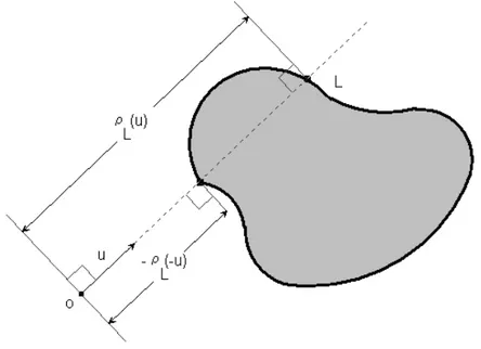
We begin this chapter with the key definition of radial function. Definition 2.1.1 (Radial function).
If L is nonempty, compact, and star-shaped at the origin o in n. Its radial function
ρL is defined by
ρL(x) = max {c : cx ∈ L} ,
for x ∈ n! {o} such that the line through x and o intersects L.
This definition, introduced by Gardner and Volčič, [18], differs from the usual definition of radial function in which the maximum is taken only over nonnegative c and shows the duality with the definition 1.1.3 of the support function defined in Chapter 1.
The radial function is positively homogeneous of degree −1, i.e., ρL(cx) =
1
cρL(x) for c > 0
and this allows us to work with the restriction of the radial function ρL to the unit
sphere, in fact we mostly use this restriction to the unit sphere. The radial function
2.1 Radial function and i-chord function 20
ρL(u) at a unit vector u ∈ Sn−1 gives the signed distance from o to the boundary of
L along the line lu, (see Figure 2.1).
Figure 2.1: The radial function
Denote by DLand SL the domain and the support of the restriction of the radial
function ρL to the unit sphere Sn−1, respectively.
A star body is a body such that ρL, restricted to SL, is continuous.
A star set is a set that is a star body in its linear hull. The class of star bodies contains the class of convex bodies.
The definition of the X-ray of a body E star-shaped at a point p can be reformulated in terms of its radial function ρE. For each u ∈ Sn−1, we have,
XpE(u) =
#
ρE−p(u) + ρE−p(−u) if p ∈ E,
$
$|ρE−p(u)| − |ρE−p(−u)| $
$ if p /∈ E. .
The notion of i-chord functions for i '= 1 arise naturally from a certain general-ization of Hammer’s problems to higher dimensions.
In fact, this has been introduced by Falconer in [11] for integer values 0 < i < n, where n is the dimension of the Euclidean space n in which the problem is handled.
2.1 Radial function and i-chord function 21
a convex body K. The i-chord functions are particularly useful when i is an inte-ger strictly between 0 and n, but they have been extended to all inteinte-ger values by Gardner in [14] and to all real numbers in [16].
Definition 2.1.2 (i-chord function).
Let i ∈ , and suppose that L is a star set in n. If i ≤ 0, we assume that o ∈ relint L
or o /∈ L. The i-chord function ρi,L of L at o is defined for u ∈ Sn−1 as follows. If
the line through o parallel to u does not intersect L we define ρi,L= 0. Otherwise, if
i '= 0, we let ρi,L(u) = # ρL(u)i+ ρL(−u)i if o ∈ L, $ $|ρL(u)|i− |ρL(−u)|i $ $ if o /∈ L . For i = 0, we define the 0-chord function of L at o for u ∈ Sn−1 by
ρ0,L(u) = # ρL(u)ρL(−u) if o ∈ L, exp$$log | ρL(u) ρL(−u)| $ $ if o /∈ L .
If p is a point in n such that L − p is a star set, then the i-chord function of L at p
is simply the i-chord function at the origin o of L − p, in symbol ρi,p,L(u) = ρi,L−p(u).
In order to better understand this definition, consider the distances from a point p ∈ n to the boundary of L along a line through p and parallel to a direction
u ∈ Sn−1. If p belongs to L, then the i-chord function of L at p gives the sum of the
ith powers of these distances or the product of these distances, according as i '= 0 or i = 0, respectively. While, if p does not belong to L, then it renders the difference (the greater less the smaller) of the ith powers of these distances or the quotient (the greater over the smaller) of these distances, according as i '= 0 or i = 0, respectively. The assumption that for i ≤ 0 the point p has to belong to the relative boundary of L or p /∈ L is necessary in order to avoid singularities.
Note that for i = 1 we retrieve the X-ray of L at p.
The analogous notion of a directed i-chord function at a point p, not in the interior of a body, can be obtained from the i-chord function by setting it equal to zero at u ∈ Sn−1 if the ray issuing from p in the direction u does not meet the body in a point other that p itself.
2.1 Radial function and i-chord function 22
Proposition 2.1.3.
Let i ∈ , and suppose that L is a star set in n. Then
ρ0,L(u) = lim i→0 % 1 2ρi,L(u) &2i (2.1) if o ∈ K and ρ0,L(u) = lim i→0exp % ρi,L(u) |i| & (2.2) if o /∈ K. Proof. ρ0,L(u) = lim i→0 % 1 2ρi,L(u) &2i = lim i→0 ' 1 2 ( ρL(u)i+ ρL(−u)i )* 2 i = lim i→0exp # log' 1 2 ( ρL(u)i+ ρL(−u)i )* 2 i + = exp lim i→0
2 log/12(ρL(u)i+ ρL(−u)i
)0 i by De l’Hopital = exp lim i→02 · 1 2 (
ρL(u)ilog ρL(u) + ρL(−u)ilog ρL(−u)
) 1 2 ( ρL(u)i+ ρL(−u)i )
= exp {log ρL(u) + log ρL(−u)}
= exp {log ρL(u)ρL(−u)}
= ρL(u)ρL(−u).
The equation (2.2) can be written in the following way.
ρ0,L(u) = lim i→0exp $ $ $|ρL(u)| i − |ρL(−u)|i $ $ $ |i| ,
2.1 Radial function and i-chord function 23
If both numerator and denominator are positive (or negative) we get
ρ0,L(u) = lim i→0exp $ $ $|ρL(u)| i − |ρL(−u)|i $ $ $ |i| = exp # lim i→0 |ρL(u)|i− |ρL(−u)|i i + by De l’Hopital = exp 8 lim i→0 (
|ρL(u)|ilog |ρL(u)| − |ρL(−u)|ilog |ρL(−u)|
)9
= exp {log |ρL(u)| − log |ρL(−u)|}
= exp 8 log |ρL(u)| |ρL(−u)| 9 .
Otherwise, if numerator is positive and denominator negative (or viceversa), we have ρ0,L(u) = lim i→0exp $ $ $|ρL(−u)| i − |ρL(u)|i $ $ $ |i| = exp # lim i→0 |ρL(−u)|i− |ρL(u)|i i + by De l’Hopital = exp 8 lim i→0 (
|ρL(−u)|ilog |ρL(−u)| − |ρL(u)|ilog |ρL(u)|
)9
= exp {log |ρL(−u)| − log |ρL(u)|}
= exp 8 log|ρL(−u)| |ρL(u)| 9 = exp # log % |ρL(u)| |ρL(−u)| &−1+ = exp 8 − log |ρL(u)| |ρL(−u)| 9 . Therefore ρ0,L(u) = exp $ $ $ $ log $ $ $ $ ρL(u) ρL(−u) $ $ $ $ $ $ $ $ .
2.2 The ith section function 24
Note that in the equation (2.1), lim i→0 % 1 2ρi,L(u) &1 i = : ρ0,L(u)
the quantity in the limit on the left is the ith mean of ρL(u) and ρL(−u), while that
on the right is the geometric mean of ρL(u) and ρL(−u).
Falconer in [9] was the first to define i-chord functions, also called generalized chord functions, for integer values of i, and gave some uniqueness results, for i ≥ 1, by use of a version of the stable manifold theorem of differentiable dynamics. Gardner in [16] generalizes the notion of i-chord function to real values of the parameter i, while Soranzo in [39] extends the definition of i-chord function to i = ±∞, when K is a convex body, by
ρ+∞,K(u) = max {|ρK(u)| , |ρK(−u)|}
and
ρ−∞,K(u) = min {|ρK(u)| , |ρK(−u)|}
and found some results about the determination of convex bodies by these functions.
2.2
The ith section function
For integer values of i, the i-chord function is closely related (via Funk theorem) to the ith section function of a convex body, the function giving the i-dimensional volumes of its intersections with i-dimensional subspaces.
Definition 2.2.1 (ith section function).
Let p ∈ n and let K be a convex body in n and let i be an integer, 1 ≤ i ≤ n − 1.
The i-section function of K at p is defined on G (n, i) by G +→ λi(K ∩ G).
The i-section function of K in a direction u ∈ Sn−1 is defined on G (n, i, u) by
G +→ λi(K ∩ G).
sub-2.3 i-chord function and ith section function 25
spaces of nand λ
ithe i-dimensional Lebesgue measure, while G (n, i, u) is the
man-ifold of all the i-dimensional affine subspaces of n parallel to the vector u.
We are in front of the following geometric problem:
« Suppose that K ⊂ n is a convex body and let p
h be some
non-collinear points (some of them are possibly at infinity). Suppose, more-over, that we are given at the points ph the ith section functions for
i ∈ {1, 2, · · · , n − 1}. Is K then uniquely determined among all convex bodies? »
The ith section functions are a particular case of the notion of dual mixed volumes introduced by Lutwak in [31] and generalized in [18]. Let L be a star set in n, and
let i ∈ be non-zero. If 1 ≤ k ≤ n − 1, the dual volume ˜Vi,k(L ∩ S) is given for
S ∈ G (n, k) by ˜ Vi,k(L ∩ S) = 1 2k " Sn−1∩S ρi,L(u)du. (2.3)
The function ˜Vi,k(L ∩ ·) is called a section function. When i = k, the function
˜
Vi,i(L ∩ ·) is called ith section function.
Observe that
˜
Vi,i(L ∩ S) = λi(L ∩ S), (2.4)
for each S ∈ G (n, i).
This means that the ith section function is nothing other than the i-dimensional X-ray of L at the origin.
Note that the relation (2.4) expresses the equivalence between the ith section function and the X-ray of order i at the origin of the body K, moreover for k = i = 1 the 1-chord function of K at a point p and the 1st section function are nothing other than the ordinary X-ray of K.
2.3
i-chord function and ith section function
In this section we state a lemma and two propositions that show the relationship between i-chord function and ith section function. For further details we refer to Gardner’s book [16]. First of all, the notion of the i-chord function is, in general, closely linked to the notion of the X-ray of order i, and this relationship is established by the following lemma.
2.3 i-chord function and ith section function 26
Lemma 2.3.1.
Let E be a body in n star-shaped at o. Suppose either that o /∈ E or that i ∈ +. If
i '= 0, then for each u ∈ Sn−1, Xi,oE(u) = 1 i <ρEi(u) + ρEi(−u) = if o ∈ E, 1 i $ $ $ $ρEi(u) $ $− $ $ρEi(−u) $ $ $ $ if o /∈ E.
If i = 0 and o /∈ E, then for each u ∈ Sn−1,
X0,oE(u) = $ $ $ $ log $ $ $ $ ρE(u) ρE(−u) $ $ $ $ $ $ $ $ .
Therefore, the X-ray of order i is the i-chord function divided by i or the natural logarithm of the i-chord function, according as i '= 0 or i = 0, respectively.
We now state the following useful proposition that gives a link between i-chord functions and ith section functions for 1 ≤ i ≤ n − 1, even if the latter is defined only for integer values of i. This result relies on Funk’s theorem [12] and is discussed in detail in [16].
Proposition 2.3.2.
Let K, K# be two convex bodies in n, and let i ∈ be such that 1 ≤ i ≤ n − 1. Then
λi(K ∩ S) = λi(K#∩ S)
for all S ∈ G (n, i), if and only if
ρi,K(u) = ρi,K!(u)
for all u ∈ Sn−1.
This observation allows us to treat the geometric problem of studying the re-construction of a convex body from X-rays or ith section functions within the more general problem of retrieving a convex body from its i-chord functions. In fact, the concept of chord function is not so appealing from the geometric point of view as much as that of section function.
The next proposition (proved in [40], Proposition 2.2) establishes an important relationship between the kth section function in direction u and the ordinary X-ray in the same direction.
2.3 i-chord function and ith section function 27
Proposition 2.3.3.
Let u ∈ Sn−1 be a fixed direction, and suppose that K and K# are two convex bodies
in n. Let k ∈ be such that 1 ≤ k ≤ n − 1. Then
λk(K ∩ S) = λk(K#∩ S)
for all S ∈ G (n, k, u) if and only if
λ1(K ∩ l) = λ1(K#∩ l)
for every line l parallel to u. Proof.
Let lu+ x ∈ G (n, k, u) be the line passing through x ∈ u⊥ and parallel to u ∈ Sn−1.
By Fubini’s theorem we have λk(Kj∩ G) =
"
G∩u⊥
λ1(Kj ∩ (lu+ x))dλk−1(x)
for j = 1, 2, and this proves the theorem in one direction.
Now, consider the mapping on G (n, k, u) such that to each G ∈ G (n, k, u) assigns the measure λk(Kj ∩ G). This is the (k − 1)-dimensional Radon transform of the
function fj(x) = λ1(Kj∩ (lu+ x)) for j = 1, 2, defined on the (n − 1)-dimensional
subspace u⊥. Since the Radon transform is injective it follows that f
1 = f2, that is
λ1(K1∩ (lu+ x)) = λ1(K2∩ (lu+ x)),
and this completes the proof.
Proposition 2.3.3 shows that, when the point source is at the infinity, the kth section function in direction u has as its counterpart the ordinary X-ray. By using Propositions 2.3.2 and 2.3.3 we can reformulate the problem in analytic form:
« Suppose that K ⊂ n is a convex body and let p
h be some noncollinear
points (some of them are possibly at infinity). Suppose, moreover, that we are given at the points ph the i-chord functions, with i ∈ . Is K then
2.4 The corresponding components 28
2.4
The corresponding components
We can establish a correspondence between components of int (K)K#), whenever
K and K#have the same i-chord function, for i > 0, at a point p. Consider two convex
bodies K and K# with the same i-chord function at a point p ∈ ∂K ∪ ∂K#. Let l be
a line through p. Then two things may happen 1. l ∩ int (K)K#) has two components;
2. l ∩ int (K)K#) is empty.
Moreover, since i > 0, l ∩ K and l ∩ K# are two closed segments which may have a
nonempty intersection and in addition no one includes the other. Definition 2.4.1 (Corresponding components).
Let K and K#be two convex bodies having the same i-chord functions at p /∈ ∂K∪∂K#.
If A is a component of int (K)K#) then we define
A#= !
z∈A
{pz ∩ int (K)K#)}! A
and we shall say that A and A# correspond to each other through p.
Observe that if A ⊂ (K !K#) then A# ⊂ (K#!K). In addition, the corresponding
components are star-shaped at p but not necessarily convex. Lemma 2.4.2.
Let K and K#be two convex bodies having the same i-chord functions at p /∈ ∂K∪∂K#.
If A and A# are two corresponding components of int (K)K#) and correspond to each
other through p then A and A# have the same i-chord functions at p.
Proof.
To simplify the notation assume that p = o. Let z be a point in A. Denote by u the direction identified by the point z, i.e. u = z
||z||, and call l the line issuing from
the origin with direction u. Since z ∈ A, A ∩ l is a segment. To see this, suppose by contrary that A = {z}, then A ∩ l = {z} and −uρK(−u) = −uρK!(−u) = {z},
but this means that z ∈ ∂K ∩ ∂K# and this contradicts the assumptions that A ⊂
int (K ! K#) Since K and K# have the same i-chord functions at o, we have
(a) $ $|ρK(u)|i− |ρK(−u)|i $ $= $ $|ρK!(u)|i− |ρK!(−u)|i $ $ (2.5)
2.4 The corresponding components 29
if o /∈ K ∪ K#, while
(b)
ρK(u)i+ ρK(−u)i = ρK!(u)i+ ρK!(−u)i (2.6)
if o ∈ K ∩ K#.
(a) Without loss of generality we may assume that o, −uρK(−u) and uρK(u) are
in that order on l as well as o, −uρK!(−u) and uρK!(u), and moreover that
0 < ρK(u) < ρK!(u) (2.7)
for every z ∈ A.
The relation (2.5) can be rewritten in the following way ρK(u)i− (−ρK(−u))i = ρK!(u)i− (−ρK!(−u))i
and from this follows that
(−ρK!(−u))i− (−ρK(−u))i = ρK!(u)i− ρK(u)i.
The last identity tells us that A and A# have the same i-chord functions.
2.4 The corresponding components 30
(b) Without loss of generality we may suppose that −uρK(−u), o and uρK(u) are
in the same order on l as well as −uρK!(−u), o, uρK!(u).
Assume also that
0 < ρK!(u) < ρK(u) (2.8)
holds for every z ∈ A.
The relation (2.6) can be rewritten in the following way ρK!(u)i− ρK(u)i = ρK(−u)i− ρK!(−u)i
and this means that A and A# have the same i-chord functions at o.
Figure 2.3
Moreover observe that, from (2.8) follows that ρK!(u)i< ρK(u)i
that is
ρK(u)i− ρK!(u)i> 0
2.4 The corresponding components 31
Now recall some useful topological preliminaries. Definition 2.4.3 (Space path-connected).
A topological space X is said to be path-connected (or pathwise connected) if there is a path joining any two points in X.
Theorem 2.4.4.
Let X and Y be topological spaces and let f : X +→ Y be a continuous function. If X is path-connected then the image f (X) is path-connected.
Proof.
Let A ⊂ X be path-connected. We want to prove that f (A) is path-connected. In fact, let y1, y2 ∈ f (A), then there exist x1, x2 ∈ A such that f (x1) = y1 and
f (x2) = y2. Since A is path-connected there exists a path γ : [0, 1] +→ X such that
γ(0) = x1, γ(1) = x2 and γ([0, 1]) ⊂ A. Now, the composition of two continuous
functions is continuous, so the function f ◦ φ : [0, 1] +→ Y is continuous and moreover (f ◦ γ)(0) = f (γ(0)) = f (x1) = y1, (f ◦ γ)(1) = f (γ(1)) = f (x2) = y2
and
(f ◦ γ)([0, 1]) = f (γ([0, 1])) ⊂ f (A) then f (A) is path-connected.
Theorem 2.4.5.
If A is a nonempty connected open subset of n then A is path-connected.
Proof.
Let x, y be two points of A and suppose that y is not reachable from x. Divide A in two subsets X and Y , where X is the set of all the points that are reachable from x, while Y contains all the points that are not reachable from x. Therefore {X, Y } is a partition of A, A = X ∪ Y with X and Y nonempty because at least x ∈ X.
and y ∈ Y . Let us show that X and Y are open. Let x∗ ∈ X ⊂ A. Since A is
open there exist an open ball B(x∗) centered at x∗ such that x∗ ∈ B(x∗) ⊂ A. Since
2.4 The corresponding components 32
Consequently x∗ ∈ B(x∗) ⊂ X. Analogously, let y∗ ∈ Y ⊂ A, then there exists an
open ball B(y∗) centered at y∗ such that y∗ ∈ B(y∗) ⊂ A. Since B(y∗) is
path-connected, every w ∈ B(y∗) is not reachable from x hence y∗ ∈ B(y∗) ⊂ Y and so
Y is open. But this contradicts our assumption because A would not be connected. Therefore Y = ∅ and A = X is path-connected.
Proposition 2.4.6.
If K and K# have the same i-chord functions at p /∈ ∂K ∪ ∂K#, and suppose that A
is a component of int (K)K#), then the set
A#= !
z∈A
{pz ∩ int (K)K#)}! A is another component of int (K)K#).
Proof.
To simplify the notation assume that p = o. It follows immediately from Lemma 2.4.2 that if z ∈ A, then A ∩ pz and A# ∩ pz are non-degenerate segment. On the
other hand, if z ∈ ∂K ∩ ∂K#, then also the other endpoint of the segment pz ∩ K
belongs to ∂K ∩ ∂K#.
We have to distinguish two cases: (a) A is between the origin o and A#;
(b) o is between A and A#.
(a) In this case pos(A) = pos(A#).
The set
U = Sn−1∩ pos(A)
is open and connected. Therefore we can represent the component A as A = 8 z : −ρK % − z ||z|| & < ||z|| < −ρK! % − z ||z|| & , z ||z|| ∈ U 9
with ρK(−v) = ρK!(−v) when v belongs to U .
Similarly, A#= 8 w : ρK % w ||w|| & < ||w|| < ρK! % w ||w|| & , w ||w|| ∈ U 9 .
2.4 The corresponding components 33
If v belongs to U then ρK(v) = ρK!(v) and moreover,
−ρK(−u) < −ρK!(−u)
if and only if
ρK(u) < ρK!(u).
Let z1, z2 ∈ pos(A) and suppose that y1, y2 ∈ A#. Then
yj = zj ||zj|| ' tjρK % zj ||zj|| & + (1 − tj)ρK! % zj ||zj|| &* for j = 1, 2. If z1 ||z1|| = z2
||z2||, then y1 and y2 are aligned and so they are the
endpoints of a segment contained in A#. Otherwise, let
xj = zj ||zj|| ' tjρK % − zj ||zj|| & + (1 − tj)ρK! % − zj ||zj|| &*
for j = 1, 2. Since A is a component, A is a nonempty connected open subset of n, then A is path-connected, therefore there exists a path x(s) joining x
1
and x2 interior to A. We may represent it with two mapping f and g given by
f : [0, 1] +→ [0, 1] and g : [0, 1] +→ U such that f (0) = t1, f (1) = t2 and g(0) = z1 ||z1|| , g(1) = z2 ||z2|| . According to these assumptions,
x(s) = g(s) [f (s)ρK(−g(s)) + (1 − f (s))ρK!(−g(s))] .
Then
y(s) = g(s) [f (s)ρK(g(s)) + (1 − f (s))ρK!(g(s))]
is a path contained in A# which connect y
1 to y2, therefore A# is path-connected
and so connected, and this implies that A# is a component.
(b) Since the origin is between A and A#, pos(A) = −pos(A#). We can follow the
2.4 The corresponding components 34
that this time the set U is given by
U = Sn−1∩ pos(A#).
With this assumption the expression of A and A# remain unchanged. Moreover,
choosing z1 and z2 in posA#, we can consider yj and xj, for j = 1, 2, in the
same way of the previous case and this completes the proof.
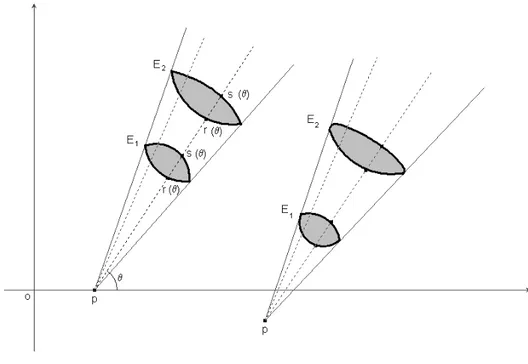
Consider two corresponding components A and A# through a point p. If A is nearer
to p than A#or, in other words, A is between p and A#, we shall say that A is “visible”
from p and write p(A) = A#, whereas if A# is nearer to p, we write p−1(A) = A#; in
Chapter 3
Determination of planar convex
bodies by i-chord functions
In this chapter our goal is to investigate the tomography of convex bodies in the plane.
3.1
i-chord functions of planar convex bodies
Lemma 3.1.1 (Cavalieri principle).
Let u ∈ Sn−1 be a direction and let E and E# be two measurable sets such that
for each line l parallel to u, l ∩ E and l ∩ E# are segments of equal length. Then
λn(E) = λn(E#).
The Cavalieri principle is substituted, in modern measure theory, by the Fubini’s theorem.
From now on we will restrict our attention to the planar case. The three-dimensional case will be treated in Chapter 4. We are not interested, in this exposition, in higher dimensions.
The two-dimensional Cavalieri principle states that if two measurable sets have the same parallel X-rays, then they have the same area.
For X-rays issuing from a point there is a substitute for the Cavalieri principle. This fact was for the first time observed and exploited by Volčič in [44], where the author introduced an appropriate measure which is preserved if two measurable sets have the same point X-rays. The idea of replacing Lebesgue measure by the measure νi
of Definition 3.1.2, which has seeds in work of Finch, Smith and Solmon [23] and of Falconer (see [11, Lemma2]), is due to Volčič. This idea has been extended by
3.1 i-chord functions of planar convex bodies 36
Gardner ([14]) to i-chord functions for i ∈ and later on the same author in his book [16] to all real values of i.
Definition 3.1.2 (The measure νk).
Let L2 be the class of bounded Lebesgue measurable subset of 2. Let l be a line
chosen as the x-axis of a Cartesian coordinate system in 2. If E ∈ L
2, define for each k ∈ , νk(E) = "" E |y|k−2dxdy.
νk is a measure on L2 and the line l will be called the base line for νk.
Observe that
ν2(E) = λ2(E).
If k > 1, then νkis a finite measure, but if k ≤ 1, then νk is a σ-finite measure in 2,
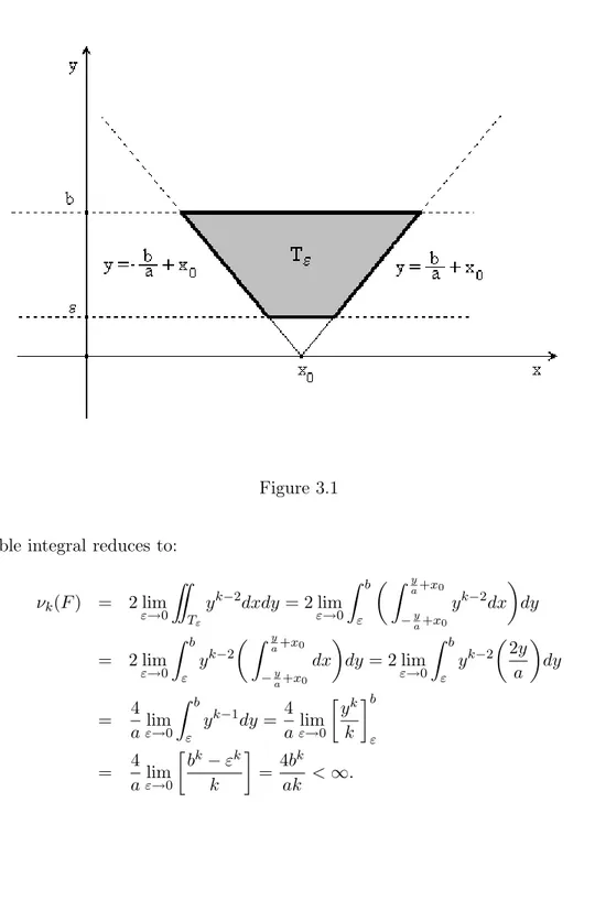
which is finite on sets having positive distance from l. Lemma 3.1.3.
The set F = {(x, y) : a|x − x0| ≤ y ≤ b}, with a > 0 has finite νk-measure for every
positive value of k. Proof.
Since the integrand f (x, y) = |y|k−2 is an unbounded function for y = 0, this is an improper integral of second kind. Moreover f is an even function therefore
νk(F ) =
""
F
|y|k−2dxdy = 2 lim
ε→0
""
Tε
yk−2dxdy where Tε is the trapezium in the first quadrant (see Figure 3.1)
Tε= > (x, y) : −y a+ x0 ≤ x ≤ y a+ x0, ε ≤ y ≤ b ? .
3.1 i-chord functions of planar convex bodies 37
Figure 3.1 double integral reduces to:
νk(F ) = 2 lim ε→0 "" Tε yk−2dxdy = 2 lim ε→0 " b ε % " y a+x0 −ya+x0 yk−2dx & dy = 2 lim ε→0 " b ε yk−2 % " y a+x0 −ya+x0 dx & dy = 2 lim ε→0 " b ε yk−2% 2y a & dy = 4 aε→0lim " b ε yk−1dy = 4 aε→0lim ' yk k *b ε = 4 aε→0lim ' bk− εk k * = 4b k ak < ∞.
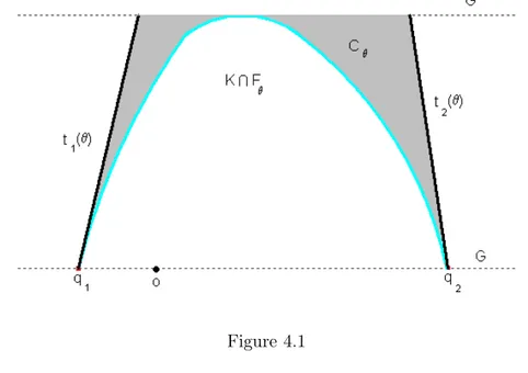
Let E1, E2 ∈ L2 with λ2(Ej) > 0, j = 1, 2. Let p = (x0, y0) ∈ 2, and suppose
that E1 and E2 are bodies star-shaped at p, with the same i-chord functions at p, for
3.1 i-chord functions of planar convex bodies 38
and that E1 is between p and E2. Let (r, θ) be polar coordinates centered at p
#
x = x0+ r cos θ r ∈ [0, +∞)
y = y0+ r sin θ θ ∈ [0, π]
. (3.1)
Let 0 ≤ α < β ≤ π, and let
Ej = {(r, θ) : rj(θ) ≤ r ≤ sj(θ), α ≤ θ ≤ β} ,
for j = 1, 2.
Since E1 and E2 have, by assumptions, the same i-chord functions at p, and
p /∈ E1∪ E2 we have that s1(θ)i− r1(θ)i= s2(θ)i− r2(θ)i (3.2) or s1(θ) r1(θ) = s2(θ) r2(θ) (3.3)
hold for α ≤ θ ≤ β when i '= 0 or i = 0, respectively. For j = 1, 2, the expression of νk in polar coordinates is
νk(Ej) = " β α " sj(θ) rj(θ) |y0+ r sin θ|k−2rdrdθ.
If i '= 0 we put t = ri and we get
νk(Ej) = " β α " sj(θ)i rj(θ)i 1 i· t 2−i i (y0+ t 1 i sin θ) k−2 dtdθ, (3.4)
while if i = 0 making the substitution t = log r we obtain νk(Ej) = " β α " log sj(θ) log rj(θ) e2t(y0+ etsin θ)k−2dtdθ. (3.5)
For the next three lemmas we have the same assumptions just described. Lemma 3.1.4.
Let i ∈ . Suppose that E1 and E2 are defined as above, with finite νi-measure and
3.1 i-chord functions of planar convex bodies 39
Proof.
If i '= 0, substituting k = i and y0= 0 in (3.4) for j = 1, 2 we get
νi(Ej) = " β α " sj(θ)i rj(θ)i 1 i · t 2−i i (t 1 i sin θ) i−2 dtdθ = " β α (sin θ)i−2 % " sj(θ)i rj(θ)i 1 idt & dθ = " β α (sin θ)i−2% sj(θ) i− r j(θ)i i & dθ. While if i = 0, substituting k = i and y0 = 0 in (3.5) for j = 1, 2 we get
ν0(Ej) = " β α " log sj(θ) log rj(θ) e2t(etsin θ)−2dtdθ = " β α (sin θ)−2 " log sj(θ) log rj(θ) dtdθ = " β α (sin θ)−2 % logsj(θ) rj(θ) & dθ
and relations (3.2) and (3.3) complete the proof.
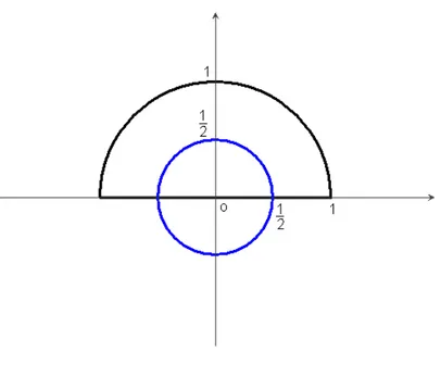
For i-chord functions at a point p we have to distinguish between equality and equality almost everywhere. This difference does not exist for convex bodies not containing p in their boundaries.
For example, let K be the upper half of the unit disk and let K# be the centered
disk of radius 1
2, (see Figure 3.2). These two convex bodies, K and K#, have 1-chord
functions at the origin equal almost everywhere, but not everywhere, since o ∈ ∂K. If the i-chord functions of two star bodies at a point p agree almost everywhere, and p is either contained in the interior of the bodies or exterior to them, then the i-chord functions at p agree everywhere. Moreover, if the point p is exterior to both bodies, then the equality of the i-chord functions at p implies that the bodies have common supporting lines through p.
Lemma 3.1.5.
Let i ∈ . Suppose that E1 and E2 are defined as above, with finite νi−1-measure
and the same i-chord functions at p = (x0, 0). Then the centroids of E1 and E2, with