Prediction Intervals for Heteroscedastic Series by Holt-Winters Methods

by Holt-Winters methods

Paolo Chirico DIGSPES Alessandria University of Eastern Piedmont, Italty

paolo.chirico@uniupo.it

Abstract The paper illustrates a procedure to calculate prediction intervals in case of heteroscedas-ticity using Holt-Winters methods. The procedure has been applied to the Italian daily electricity prices (PUN) of the year 2014; then the prediction intervals have compared to those provided by an ARIMA-GARCH model. The intervals obtained with HW methods have been very similar to the others, but easier to calculate. Moreover, the HW procedure is more flexible in dealing with periodic volatility as proved in the case study.

Key words: Holt-Winters methods, heteroscedasticity, prediction intervals.

1 Introduction

The Holt-Winters (HW) methods are forecast methods grounding on recursive formulas for updat-ing the structural components of time series: the local mean level, Lt; the local trend, Tt; the local

seasonal index, It, if the series is affect by periodic effects. According to the composition model of

the structural components, the HW methods can be either additive or multiplicative. In the first case, when a new observation, ytbecomes available, the forecast of yt+k, denoted bybyt(k), is:

b

yt(k) = Lt+ kTt+ It+k−hS h= int(k/S) + 1 (1)

after having updated the structural components:

Lt = α(Yt− It−s) + (1 − α)(Lt−1+ Tt−1) (2)

Tt = β (Lt− Lt−1) + (1 − β )Tt−1 (3)

It = γ(Yt− Lt) + (1 − γ)It−S (4)

where 0 ≤ α, β , γ ≤ 1 are smoothing coefficients, and S is the length of the seasonal cycle. The additive HW provides optimal forecast if the series derives from a SARIMA process of order (0, 1, S + 1)(0, 1, 0)S(Yar and Chatfield, 1990)1.

Post print copy

1_{Instead, the multiplicative HW is not optimal for any linear process. In case of multiplicative composition of the} structural components, it is worthwhile to apply the additive HW to the log-serie.

Originally, the HW methods were not thought for prediction intervals (PIs), but over time, some authors have proposed ways to get PIs. The proposal of Yar and Chatfield (1990) for the additive method allows to get the same PIs of the equivalent SARIMA model. They define the k-steps-ahead prediction error as:

et(k) = k−1

∑

i=0

viet+k−i (5)

where et= yt−byt−1(1) is the one-step-ahead (OSA) prediction error, and:

vi=    1 i= 0 α + iα β i6= 0, S, 2S, ... α + iα β + (1 − α )γ i= S, 2S, ... (6)

If the OSA prediction errors are uncorrelated and Gaussian N(0, σ2), the k-steps-ahead prediction intervals, at 1 − θ confidence level, is:

b yt(k) ± z(θ /2) p PMSEt(k) (7) PMSEt(k) = σ2 k−1

∑

Nevertheless this proposal assumes the OSA prediction errors are homoscedastic, that is not realistic in some cases like electricity prices (see Section 3).

2 An HW method for heteroscedastic series

Let’s suppose the OSA prediction errors are heteroscedastic, and the volatility level of them, denoted by Ht, is only locally approximative constant. Following the criterion of the Exponential Smoothing,

the update of the volatility level may be formulated as:

Ht = λ et2+ (1 − λ )Ht−1 (9)

where 0 ≤ λ ≤ 1 is a smoothing coefficient. According to the criterion:σb

2

t+1= Ht, the volatility forecasts are:

b σt+12 = λ e2t+ (1 − λ )σb 2 t (10) b σt+k2 =σb 2 t+1 k= 2, 3, ... (11)

The equation (10) is known in Statistical Process Control as Exponentially Weighted Moving Vari-ance, EWMV, (Harris, 1993). It is formally similar to the IGARCH model, but there are conceptual differences: the IGARCH model, as well as all models of GARCH family, shapes the conditional heteroscedasticity of homoscedastic processes (Engle and Bollerslev, 1986); the method (10) treats a general heteroscedasticity where the volatility can be viewed as a stochastic process. Then the method (10) is conceptually more similar to the methods for stochastic volatility (Taylor, 1994).

Taking into account the (11), under the assumption of uncorrelated OSA prediction errors, the PMSEt(k) becomes:

PMSEt(k) = k−1

∑

∑

where the coefficients vis have been defined in (6).

This formula is very similar to (8), but presents a fundamental difference: now the PMSEt(k)

depends on the last predicted volatility; that means more accurate PIs in case of heteroscedastic e2 t.

Periodic Volatility In case of seasonal data, heteroscedasticity can follow a seasonal pattern (sea-sonal volatility): e.g. daily electricity prices present sea(sea-sonal patterns in the price levels and in the price volatilities. A way to deal with such a case in GARCH framework was proposed by Koopman et al. (2007) who suggested to scale volatility by means of seasonal factors. According to that idea, but remaining in HW framework, the method (10) should be changed in the multiplicative following HW method2:

b

σ_t+k2 = Ht· Xt+k−hS h= int(k/S) + 1

Ht = λ (e2t/Xt−S) + (1 − λ )Ht−1 (14)

Xt = λx(e2t/Ht) + (1 − λx)Xt−S

where Xt represents the seasonal effect on volatility, and 0 ≤ λx≤ 1 is the corresponding smoothing

coefficient.

Note that now the formula (12) cannot be reduced into the formula (13) becauseσ_bt+k2 is only periodically constant, then PMSEt(k) presents cyclical fluctuations.

The smoothing coefficients The value (1 − λ ) can be viewed as the persistence degree of volatility: when (1 − λ ) = 1, volatility (or its level) is constant (max persistence); when (1 − λ ) = 0, each variance/level does not depend on any previous variances/levels (null persistence). Similarly, (1 − λx) = 1 means that the seasonal pattern on volatility is constant, and (1 − λx) = 0 means that there

is no seasonal pattern on volatility.

The smoothing coefficients, α, β , γ, λ and λx, could be chosen minimising the following sum:

∑

where ut= et/σt are the standardised OSA prediction errors.

If ut ∼ N(0, 1), the criterion (15) is equivalent to the maximum likelihood, but should not be

viewed as an estimation method. Indeed, according to the theory of HW methods, the smoothing coefficients are not process parameters, but instruments to perform time series forecasting. Never-theless, in case of financial prices, the prediction standardised errors are generally leptokurtic/heavy tailed like standardised Student’s t-distributions: tvp(v − 2)/v. In that case, it is more appropriate to

minimise the following sum:

∑

u2_t v− 2)

v+1_{] (16)}

where v are the degrees of freedom of the Student’s distribution3.

2_{Here the multiplicative HW should be preferred to the additive one because it avoids negative values for volatility} forecasts.

3_{Minimizing the sum (16) is nearly equivalent to the maximum likelihood in case of Student’t distribution (Bollerslev,} 1987).

3 Prediction Intervals for the Italian PUN

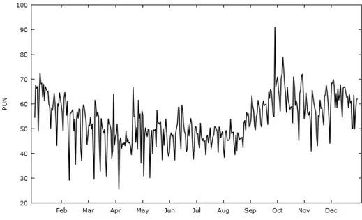
We have considered the series of the daily electricity price (PUN), cleared by the Italian wholesale electricity market in 2014. As all daily electricity market prices, Italian PUN is characterized by strong seasonality affecting the price level and price volatility too (Figure 1). On the series we have calculated one step ahead prediction intervals using the method described in the previous sections, and using a suitable ARIMA-GARCH model. Then we have compared the results obtained with both approaches.

Fig. 1 The Italian PUN in 2014

3.1 The HW approach

Since the presence of spikes and jumps makes the standardised prediction errors of electricity prices strongly leptokurtic, the smoothing coefficients of the HW method have been chosen minimising the sum (16). Table 1 reports the optimal values of the smoothing coefficients, the degree of freedom and the standard deviation of the OSA prediction errors (RMSE)4.

We can note that the smoothing coefficients present some interesting features: β = 0 means that the price level does not present any locally persistent drift; γ = 0 means that the seasonal effects on the price level are periodically constant (deterministic seasonality); λx= 0 means that the seasonality

on the volatility is deterministic too5_{. Finally, the low value of the degree of freedom (7.4) confirms}

the assumption of leptokurtic standardised prediction errors.

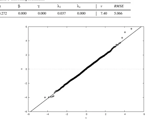
We have compared the standardized prediction errors, ut, to the standardised Student’ t-distribution

with 7.4 degrees of freedom by means of the quantile-quantile plot (Figure 2).

4_{The optimal values are reported without inferential information (standard errors, p-values, etc.) because the} coeffi-cients are not interpreted here as process parameters.

Table 1 Smoothing coefficients

α β γ λ1 λx v RMSE

0.272 0.000 0.000 0.037 0.000 7.40 5.066

Fig. 2 Q-Q plot of the standardised errors vs standardised Student’s t

We can note that the uts correspond almost well to the theoretical distribution except some errors

at the distribution extremities. That is due to the presence of spikes and jumps which cannot be consistent with the other data.

Therefore the one-step ahead prediction intervals (at 1 − θ confidence level) have been calculated with the following formulas:

LB: PU Nˆ t(1) − tθ /2∗ p PMSEt(1) (17) U B: PU Nˆ t(1) + tθ /2∗ p PMSEt(1) (18)

where t_{θ /2}∗ is the θ /2-th percentile of the standardised Student’s t distribution with 7.4 degrees of freedom.

3.2 The ARIMA-GARCH approach

We have repeated the study in 3.1 using an ARIMA-GARCH model. Similar to the method illustrated in the previous subsection, we have fitted the PUN series with an ARIMA-EGARCH model6with daily regressors (dj) and Student’s standardised errors (ut):

6_{We have chosen an EGARCH model to avoid the risk of negative variance because that risk is high including seasonal} regressors in classic GARCH model.

zt= ∆dPU Nt= µt+ εt εt= σtut ut∼ tv p (v − 2)/v µt= δ + p

∑

∑

∑

∑

∑

∑

More specifically awe have identified an ARIMA(6,1,0)-EGARCH(1,1) model with daily regres-sors, that we have estimated using the GIG package of Gretl (Lucchetti and Balietti, 2016). For space reasons, we don’t report here all the estimation output of the model, but only the standard deviation of the OSA prediction errors, RMSE = 5.062. This statistic is practically equal to one of the HW approach, that means the HM method fits the series as good as the ARMA-EGARCH model.

Finally, we have calculated the PIs of PUN series in the period September, 2014-December, 2014 using both methods (Figure 3). Although both intervals capture the 90% of the series in the period, the intervals may be quite different some days. Actually the interval by ARMA-EGARCH model (thin line) seem more sensitive to spike and jumps than one by HW methods does (thick line); this characteristic is typical of EGARCH models because outliers (jumps and spike) produce exponential effects on volatility. On the other hand, the HW procedure provides an interval whose width is quite regular: the seasonality on volatility is periodically constant (λx= 0), and the non-seasonal volatility,

Ht, is quite smoothed (λ = 0.037).

4 Final Considerations

The presence of heteroscedasticity is one of the reasons for preferring ARIMA-GARCH models to HW methods. Nevertheless heteroscedasticity can be treated by HW methods, if some adjustments are taken; the paper illustrates a method to do it. The method has been applied to a case study, and the PIs obtained with this method have been similar to the those provided by an ARIMA-EGARCH model; some days the HW procedure seems to work better than ARIMA-EGARCH model too. The most considerable strengths of using HW methods are the ease-of-use and the ability of dealing with several type of heteroscedasticity: stochastic volatility, periodic stochastic volatility, periodically constant volatility. On the other hand, the weakness is that the HW methods are optimal only for specific ARIMA processes although works quite well with a lot of real processes; moreover the HW procedure does not deal with the issue of asymmetry. Nevertheless other versions of the method above-illustrated are possible, and it is our intention to check them.

References

Bollerslev, T. (1987). A conditionally heteroskedastic time series model for speculative prices and rates of return. The review of economics and statistics, 69(3), 542–547.

Chirico, P. (2016). Which Seasonality in Italian Daily Electricity Prices? A Study with State Space Models. In Alleva, G., Giommi, A. (Eds.): Topics in Theoretical and Applied Statistics, 275–284. Springer.

Engle, R. F., Bollerslev, T. (1986). Modelling the persistence of conditional variances. Economet. Rev., 5 (1), 1–50.

Koopman, S. J., Ooms, M., Carnero, M. A. (2007). Periodic seasonal Reg- ARFIMA- GARCH models for daily electricity spot prices. J. Am. Stat. Ass., 102(477), 16–27.

Lucchetti, R. J., Balietti, S. (2016). The gig package. Package Guide of Gretl.

MacGregor, J. F., Harris, T. J. (1993). The exponentially weighted moving variance. Journal of Qual-ity Technology, 25(2), 106-118.

Taylor, S. J. (1994). Modeling stochastic volatility: A review and comparative study. Mathematical finance, 4(2), 183-204.

Yar, M., Chatfield, C. (1990). Prediction Interval for the Holt-Winters forecasting procedure. Int. J. Forecast., 6, 127–137. North-Holland