Time Sensitive Networks: analysis, testing, scheduling and simulation

(1)

Alma Mater Studiorum · Università di Bologna

SCHOOL OF ENGINEERING AND ARCHITECTURE DEPARTMENT OF ELECTRICAL, ELECTRONIC AND INFORMATION ENGINEERING "GUGLIELMO MARCONI" (DEI)

MASTER DEGREE IN AUTOMATION ENGINEERING 8891

GRADUATION THESIS in

MECHATRONICS SYSTEMS MODELING AND CONTROL M

TIME SENSITIVE NETWORKS:

ANALYSIS, TESTING, SCHEDULING

AND SIMULATION

CANDIDATE: SUPERVISOR:

Luca Cedrini eminent prof. Alessandro Macchelli

CO-SUPERVISORS: eng. Stefano Gualmini eng. Marco de Vietro

Academic year

2019/2020

Session

(2)

(3)

Ringraziamenti

Iniziamo dalla fine. Desidero ringraziare i miei correlatori, Stefano Gual-mini e Marco De Vietro, per avermi guidato e supportato nel mio lavoro durante il tirocinio. Ringrazio anche il mio relatore, il professor Alessandro Macchelli, che si è sempre mostrato gentile e disponibile.

Ulteriori ringraziamenti vanno ai miei compagni di avventura di questi anni universitari, che sono diventati a tutti gli effetti miei amici. Da quelli magistrali, Andrea, Lori, Giova, Eusebio, Ros, Martina e Baruz, a quelli con cui ho condiviso solo la triennale, Steve, Mula, Fre e Ilaria. Sono sicuro che, anche se prenderemo strade diverse, riusciremo sempre a ritrovarci.

Degli anni del liceo voglio ricordare in particolare Nick e Giulia. Ringrazio anche Sici e Benuz, con la speranza di poter presto festeggiare come si deve da Caruso.

Ringrazio poi gli amici di una vita, con cui ormai sono di famiglia sin da quando eravamo bambini: Balbo e Mattia. E non c’è davvero bisogno di aggiungere altro.

Finiamo dall’inizio. Ringrazio la mia sempre presente famiglia per avermi cresciuto ed educato. Ringrazio i miei nonni, Alfredo ed Elena, Enzo e Marisa, ringrazio i miei zii, Andrea e Morena, e ringrazio i miei genitori e mia sorella, Marco, Lucia ed Elena.

È senz’altro grazie ad ognuno di voi che sono riuscito a raggiungere questo traguardo.

(4)

Abstract

The industrial automation world is an extremely complex framework, where state-of-the-art cutting edge technologies are continuously being re-placed in order to achieve the best possible performances.

The criterion guiding this change has always been the productivity. This term has, however, a broad meaning and there are many ways to improve the productivity, that go beyond the simplistic products/min ratio.

One concept that has been increasingly emerging in the last years is the idea of interoperability: a flexible environment, where products of different and diverse vendors can be easily integrated togheter, would increase the productivity by simplifying the design and installation of any automatic system.

Connected to this concept of interoperability is the Industrial Internet of Things (IIoT), which is one of the main sources of the industrial innovation at the moment: the idea of a huge network connecting every computer, sensor or generic device so as to allow seamless data exchange, status updates and information passing.

It is in this framework that Time Sensitive Networks are placed: it is a new, work-in-progress set of communication standards whose goal is to provide a common infrastructure where all kinds of important data for an industrial automation environment, namely deterministic and non determin-istic data, can flow.

This work aims to be an initial step towards the actual implementation of the above-mentioned technology. The focus will therefore be not only on the theoretical aspects, but also on a set of practical tests that have been carried out in order to evaluate the performances, the required hardware and software features, advantages and drawbacks of such an application.

Keywords: Time Sensitive Networks (TSN), Industrial Internet of Thi-ngs, Industry 4.0, industrial communication

(5)

Abstract

Il mondo dell’automazione industriale è un ambiente estremamente com-plesso, dove nuove e innovative tecnologie vengono continuamente impiegate al fine di ottenere le migliori prestazioni possibili.

Il criterio guida di questo cambiamento è sempre stato la produttiv-ità. Questo termine ha tuttavia un largo significato, e ci sono molti modi di incrementare la produttività, che vanno oltre il semplicistico rapporto prodotti/min.

Un concetto emergente negli ultimi anni è quello di interoperabilità: creare un ambiente flessibile, caratterizzato da una facile integrazione di dispositivi di diversi produttori, aumenterebbe la produttività semplificando il lavoro di progetto e installazione di qualsiasi sistema automatico.

Collegato al concetto di interoperabilità c’è l’Industrial Internet of Things (IIoT), che è una delle principali fonti di innovazione industriale al momento: l’idea di una grande rete che mette in comunicazione calcolatori, sensori e ogni generico dispositivo per permettere un continuo scambio di dati, aggior-namenti e passaggio di informazioni.

È in questo contesto che si collocano le reti TSN: si tratta di un nuovo (ancora in via di sviluppo) gruppo di standard di comunicazione che mirano a fornire un’infrastruttura comune dove tutte le tipologie di dati di interesse industriale, soprattutto quelli deterministici e non deterministici, possono circolare.

Questo lavoro di tesi si propone di essere un passo iniziale verso la conc-reta implementazione della sopracitata tecnologia. Pertanto l’attenzione sarà concentrata non solo sugli aspetti teorici, ma anche su una serie di test pratici che sono stati svolti per valutare le prestazioni, l’hardware e il software richi-esti, i vantaggi e gli svantaggi di una tale applicazione.

Parole chiave: Time Sensitive Networks (TSN), Industrial Internet of Things, Industria 4.0, comunicazione industriale

(6)

(7)

4.2 Implementation of No-wait packet scheduling on MATLAB . 140 4.2.1 TimeTabling . . . 141 4.2.2 NWPS_Heuristic . . . 143 4.2.3 Schedules . . . 144 4.2.4 Multi-objective optimization . . . 146 4.2.5 Performance . . . 147 4.3 Test simulations . . . 151 4.3.1 Simple network . . . 151 4.3.2 Generic network . . . 156 4.3.3 Final considerations . . . 159 5 Conclusions 163 5.1 Summary . . . 164 5.1.1 Analysis . . . 164 5.1.2 Testing . . . 165 5.1.3 Scheduling . . . 166 5.1.4 Simulation . . . 167 5.2 Future developements . . . 168 5.2.1 Long-term objectives . . . 168 5.2.2 Short-term objectives . . . 169 Bibliography 170

(9)

List of Figures

1.1 TSN testbed at the Hannover Fair, 2018 . . . 18

1.2 machine-to-machine communication . . . 19

2.1 Structure of a packet . . . 24

2.2 An example of a network . . . 27

2.3 Comparison between two protocol stacks . . . 32

2.4 An example of the active layers in a transmission . . . 35

2.5 Characteristics of the four industrial revolutions . . . 37

2.6 Smart factory . . . 38

2.7 Automation pyramid . . . 40

2.8 IT support . . . 41

2.9 OPC UA client . . . 42

2.10 OPC UA meta model . . . 43

2.11 Main TSN standards . . . 44

2.12 Key elements of TSN . . . 45

2.13 Principle scheme of PTP . . . 47

2.14 Time Aware Shaper . . . 49

2.15 The use of a Guard Band . . . 51

2.16 System’s configuration . . . 54

2.17 The computed schedule . . . 55

2.18 Example of CBS for one queue . . . 57

3.1 Setup for the tests . . . 69

3.2 Setup for the tests . . . 70

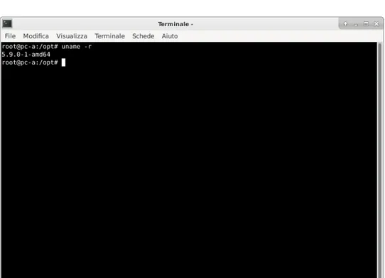
3.3 pc-a and its kernel version . . . 72

3.4 Working frequencies of the cores . . . 73

3.5 A typical graph of Wireshark . . . 74

3.6 Master’s ptp4l . . . 77

3.7 Master’s phc2sys . . . 77

3.8 Slave’s ptp4l . . . 78

3.9 Slave’s phc2sys . . . 78

3.10 Test in the master . . . 80

(10)

3.12 The time aware shaper . . . 81

3.13 Linux’s output interface . . . 82

3.14 Default queueing discipline . . . 83

3.15 A piece of code from sample-app-taprio.c . . . 89

3.16 A piece of code from sample-app-taprio.c . . . 90

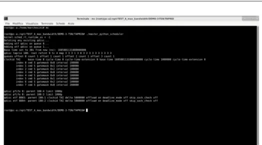
3.17 Output of the tc script . . . 93

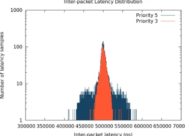
3.18 Histogram of the interpacket latency . . . 93

3.19 Zoom of Fig.3.18 . . . 94

3.20 Wireshark’s graph . . . 94

3.21 First test with MQPRIO . . . 96

3.22 Second test with MQPRIO . . . 97

3.23 Wireshark of the second test with MQPRIO . . . 97

3.24 Test with PFIFO_FAST . . . 99

3.25 Second test with TAPRIO . . . 100

3.26 Zoom of Fig. 3.25 . . . 101

3.27 Wireshark of the second test with TAPRIO . . . 101

3.28 Credit based shaper . . . 103

3.29 Wireshark of the first test with CBS . . . 103

3.30 Wireshark of the second test with CBS . . . 104

3.31 Configuration file for kernel 5.8 . . . 106

3.32 Configuration file for kernel 5.9 . . . 106

3.33 Currently loaded kernel modules . . . 107

3.34 Output of sample-app-taprio.c . . . 108

3.35 Test with the switch . . . 109

4.1 Comparison between different simulation methods . . . 116

4.2 The SimEvents library . . . 119

4.3 Configuration of a generation block . . . 123

4.4 Configuration of a generation block . . . 124

4.5 Input port . . . 126

4.6 Output port . . . 127

4.7 Schedule . . . 127

4.8 A three ports switch . . . 129

4.9 Collected data . . . 130

4.10 Generic network . . . 131

4.12 Measured interpacket latency . . . 134

4.13 Zoom of the interpacket latency . . . 134

4.14 Measured TSN latencies . . . 135

4.15 Measured best effort latencies . . . 135

4.16 Zoom of the best effort latencies . . . 136

4.17 Experimental setup . . . 137

4.18 Latencies for TSN packets . . . 138

(11)

4.20 Outputs of the function: 1 . . . 147

4.21 Outputs of the function: 2 . . . 148

4.22 Outputs of NWPS_Heuristic_mo . . . 149

4.23 Latencies for TSN packets . . . 151

4.24 Simple network . . . 152

4.25 Taskset . . . 152

4.26 Results of the simulation . . . 153

4.27 Schedule and generation . . . 154

4.29 Results about the generic network . . . 157

4.30 Average waiting times . . . 157

(12)

(13)

Chapter 1

Introduction

Overview on the main communication techniques in

industrial automation

Automatic machines are the core of any industrial plant: they are designed in such a way to be able to work autonomously for as long as possible. The idea is to let the machine work whitout any need of human intervention, which definitely increases productivity, lowers the costs for the staff and the risks associated with any industrial environment.

This means, though, that every action, every step of the productive pro-cess must be integrated togheter, creating a system that pertains several different domains: mechanical, electrical, electronic, pneumatic and so on. Also, devices belonging to the same automatic machine, that handles the same productive process, may be placed dozens of meters apart and still need to communicate or be coordinated with the highest of the precisions, in order to maximize the efficiency.

Flexibility and interoperability also play an important role in modern automation. Market’s needs often require to be able to quickly change the configuration of the machine, the format of the product or also to build even more complex systems out of several automatic machines. It is fundamental, therefore, to start from the design to take into account all the features and the future challenges that the system is going to face, and provide it with the necessary technology to to survive the test of time and make it a reliable and durable product.

As we said, industrial plants are made of numerous different devices that work in the same environment and generally tend to modify it. Automatic machines, in particular, are characterized by a high level of planning and design of the tasks for every device by which they are composed, which implies an extreme level of synchronization.

Clearly this couldn’t be done if the devices were all mute and unable to communicate one with the other. There has to exist at least one channel of

(14)

communication through which they can pass information, data, status and many other working parameters.

The trivial example is represented by the system bus, which is a link connecting all the devices of an automatic machine, starting from the main drives up to the last sensor, to the main control logic, i.e. the PLC. In this particular -yet very close to our framework- example, the communication channel works as a collector of all the operating data from the environment (sensors measurements, control inputs from the HMI, other signals of various kinds) and passes them to the computing unit so that it can compute the control signals for the next cycle; then those control signals flow through the same link to the different destinations in the plant.

In an industrial environment there exists another whole level of commu-nication, that is called Enterprise Resource Planning. ERP is a software sys-tem that utilizes a centralized database that contains all the necessary data in one location. The data are generated from the transactions produced by every process enabled by the ERP system. This database is shared across multiple departments to support multiple functions. The shared information allows for easy metric reporting and faster implementations of tasks, such as orders, marketing and bookkeeping. In essence, an ERP system automates processes across departments and helps to streamline common functions such as inventory management, order fulfillment, and order status.

These two systems coexist in most of the productive plants and basically define two different sets of information models, source and destination de-vices; but they are both needed in order for the whole plant to work properly and to increase the efficiency. As a result, a massive load of information has to be sent and delivered, every second, throughout the whole factory.

One major problem of this approach is that, potentially, a single device may have to communicate to a large set of other devices, possibly not of the same type and even produced by different vendors. Therefore it is required that all the devices act following some sorts of routine or protocol, both hardware and software, when interacting with another device of the system. This in oder to ensure that every datum that is sent into the network can be decripted and understood by everyone who is interested in it.

That’s not an easy task because, as we said, the automation industry is a mix of all kinds of technologies and devices; however several entities and organizations have already begun to develop standards and protocols useful not only in the automation field. Among the most important ones there are the International Organization for Standardization (ISO), the Institute of Electrical and Electronic Engineers (IEEE) and the OPC Foundation. Their work deals with different aspects of the industrial communication that we will study more in detail in the next chapters.

Going back to the examples of ERP and the system bus, it is important to highlight that there is a fundamental difference between these two com-munication models. It consists in the kind of data and in the guarantees

(15)

that such data have or do not need to have.

As we discussed before, an automatic machine relies on the strong syn-chronization between its elements. To do that, the signals to and from the main control unit must be delivered as fast as possible. Mere speed, though, is not the most important feature required: determinism is. We are talking about a deterministic message when the message has guaranteed delivery times, with bounded and limited jitter. This means that we are able to compute and guarantee, a priori, that every instance of the message will not break the deadlines that have been assigned to it in terms of latency and intermessage latency (i.e. the time that passes between the send and the delivery and the time that passes between two consecutive deliveries). De-terminism does not imply speed nor efficiency, but rather that even in the worst possible case we are sure about the limits of some functional parame-ters; it is achieved by reducing the randomness that naturally characterizes the physical processes.

On the other hand, the kind of data that an ERP system deals with does not have any needed guarantees about the delivery times. If the information about the productivity of a certain machine, that has to be stored in order to keep track of the performances of the plant, gets delivered to the server with a delay of some milliseconds due to network’s congestion, it is not a big deal. Instead, if the photocell sensor fails to send in time to the PLC the information about the product passing in front of it, the actions linked to this event do not get triggered, the machine loses its synchronization and as a consequence the product has to be discarded, since it hasn’t been treated properly.

The previous are two simple examples that aim at passing the idea that some messages, and in particular their temporal characteristics, are neces-sary for the correct behavior of the plant, while for other messages it does not really matter: delays certainly affect the quality of service but do not compromise in any way the operations. We usually refer to the first kind of messages as time sensitive messages, while the second class is called best effort: we try to achieve the best possible performance, but without any guarantee.

So we have seen that a large amount of data has to flow accross the plant, some with “constraints” on their delivery time and some without. The major problem is that if we use a single standard switched network as a mean for all these messages to flow, it is highly unlikely that we can guarantee the delivery time of any message. This result is mostly due to the quantity and the nature of the best effort data: they are in fact messages with very variable dimensions and rate, and they are generally many orders of magnitute more numerous with respect to the time sensitive messages. The danger is that at some point the network will become congested because too high a number of messages has been sent in a small amount of time, and the resources of the network cannot satisfy all the requests in the usual amount of time. The

(16)

victims, namely the messages that are going to face an inevitable delay, can be anyone, and there is really no way to predict when or where this scenario will take place. Time sensitive messages will be enqueued in some router along their path towards the destination, behind some best effort messages that got there first; and they will have to wait for the queue to get empty before they can leave it and reach the destination. As one can imagine, it is easy to lose control over what happens and leave things to randomness.

The most widespread solution to this problem is to use two, or more, separate networks, each one dedicated to a particular category among the ones described before. So we have a whole network where only enterprise information flows towards the different departments of the plant, and we have the local networks in the automatic machines that let every component have a “protecte” communication channel with its PLC, namely the system buses. System buses are different from a generic network because we need to add some features to make them real-time compatible: those features in general involve reducing the efficiency, the performances or the degrees of freedom in order to gain something in the determinism area.

The advantage of this approach is obviously that we can avoid distur-bances on the time sensitive messages by simply eliminating any other mes-sage from the network. But this is also kind of a drawback: the fact that we use separate networks in the same plant prevents us from being able to communicate from any device to any other device. Solutions to bridge the two networks in a way that does not affect the properties of the buses exist but are expensive and pretty impractical. In a world where the idea that “everything is connected” and “everything is online” is progressively emerg-ing with the Industrial Internet of Themerg-ings and Industry 4.0, this perspective seems a bit limiting and old.

That’s where Time Sensitive Networks come into play.

A new technology with new possibilities

Time Sensitive Networks is the name of a series of standards that are being developed by the Institute of Electrical and Electronic Engineers that aim at a better integration of all the traffic classes in the industrial communication framework.

The key idea is to exploit some new mechanisms and routing strategies in order to re-gain control over what happens in large and possibly congested networks. As we said earlier, the fact that usually standard networks are flooded with huge amounts of messages makes it very hard to predict and compute worst case delivery times for any message. Therefore we have to apply a classical tradeoff: we need to lose something in terms of performances in order to be able to impose from the outside some boundary to the latency. That’s what has been done in fielbuses, in order to guarantee that every

(17)

message flowing in the link will be delivered in time. The real innovation about TSN is that we can choose, a priori, which entities are going to be limited and which ones are going to be left free, subject to the randomness of the network.

The potential of this concept is huge: first of all, it allows us to keep the vital functions of the network for the time sensitive messages, granting that every sensor measurement or control signal will reach its intended destination before its deadline. Moreover, and that’s the great innovation, it allows us to use one, unique, large-scale network as a mean for all the messages in a plant or factory. Connecting every single device with rest of the industrial world makes the communication system cutting edge and compliant with the new trends of Industry 4.0.

Compared to the classical fieldbuses, these new techniques bring some remarkable advantages. Increased throughput, performances and efficiency, but most importantly a level of interoperabilty never seen before in this area, as this technology will be completely vendor-independent, and therefore render every device capable by construction of communicating effortless with any other device. At least on the physical level; that’s because every device also needs to know which is the format of the data that it is reading. TSN only provides a layer 2 common infrastructure, meaning that we are able to physically transmit every message from any device to any other device. But how the messages are built and read it is up to the sender and the receiver, respectively.

Let’s give a trivial example. Let’s suppose that a drive needs to send to a PLC its measurements about the current position of the shaft, picked up by its integrated encoder. If the drive records, for some reason, the value using the ASCII standard and the PLC reads the message considering the received value as an unsigned integer, the two values will never correspond, making the message itself useless, even if delivered right on time.

The scenario just depicted normally does not occur because the commu-nication networks of automatic machines are very limited in size, allowing to know precisely which devices need to intercommunicate and to adjust conse-quently their communication protocols. But the degrees of freedom offered by TSN allow, as we said, to potentially put in communication literally ev-erything. At this point it becomes tough to take into account all the possible devices that could share information and provide them all with a suitable protocol. As a matter of fact, in the previous example it was not specified which PLC was the destination of the position, indeed because we could con-nect a sensor of a certain automatic machine with the PLC of another one; maybe it is the PLC of the downstream machine that has to take as input the flow of incoming products and needs to know their position on the conveyor belt. Or maybe it could even be the enterprise server, which is supposed to record the operational parameters of every device in the plant, allowing for a more sofisticated and complete statistical analysis and data tracking. In

(18)

this last case, then, the message is not supposed to meet deadlines in terms of latency but it does not really matter: as long as we have configured the network in the right way, it will be treated as deterministic or as best effort according to the specific needs of the receiver.

The OPC Foundation has been active for some time on this field, produc-ing standard protocols for industrial communication. It has also contributed to the TSN topic, among other organizations such as Kalycito and Fraun-hofer, by developing some testbeds involving deterministic data expressed in a standardized and universal format. Particular reference to [1], where a practical test exposed at the 2018 Hannover Fair is described.

Figure 1.1: TSN testbed at the Hannover Fair, 2018

They tested the real time communications between two industrial PCs directly connected through an ethernet cable. They were able to verify that adopting TSN could grant bounded and deterministic jitters in terms of latencies for the messages, while using the standard network’s services the value of the jitter could become quite unpredictable and not controllable.

Putting aside, for the moment, the discussion about ERP and the higher levels of the automation pyramid, let’s just consider the productive process, made by one or more coordinated automatic machines. What could be some possible use cases of an actual implementation of TSN in this limited area? The main application in certainly a real-time machine-to-machine com-munication (M2M). M2M comcom-munication -two machines communicating with-out human interaction- is reinventing manufacturing by enabling data to be

(19)

shared across different control and analytical applications to derive superior operational efficiencies. TSN enhances M2M communication by connect-ing previously unconnected proprietary controllers. This is made possible through a network of TSN machines (TSN-compliant end points) connected through TSN-enabled switches. M2M communication can enable remote management, operation of equipment/devices through cellular point-to-point connections.

Figure 1.2: machine-to-machine communication

Figure 1.2 shows a production cell with a supervisory PLC coordinating communication across four different TSN machines. Another example of M2M communication can be PLCs communicating with other controllers, conveyor belts, and other control equipment (at the same network layer) to regulate or monitor the production of a product.

TSN could also be exploited in robotic applications. An industrial robot is a programmable, mechanical device used in place of a person to perform dangerous or repetitive tasks with a high degree of accuracy. Based on the operating environment, industrial robots can be classified as fixed (robotic arms), mobile (autonomous guide vehicles) and collaborative (pick and place robots). A key challenge in robotics is the absence of a standard commu-nication protocol. Robotic manufacturers must support many customized protocols, which can lead to increased integration times and costs. Since modern robotics integrates artificial intelligence (AI), machine vision, and predictive maintenance into one system, there is a need for sensors and ac-tuators to stream high bandwidth data in real time. A common solution is to use a specific channel for real-time control (similar to the system buses) and a separate one for higher bandwidth communications (TCP/UDP), just like we highlighted before. For applications that generate high bandwidth traffic (100 MB/s to 1 GB/s), using two separate communication channels becomes inefficient. TSN provides a shared communication channel for high

(20)

bandwidth traffic and real-time control traffic.

Lastly, motion control applications have strict delay requirements to en-sure that real-time data transmissions can support workload demands. Mo-tion control spans various industrial market segments (discrete industries, process industries, power industry, etc.) and supports dedicated applications such as PLC controllers. Other use cases include controlling the velocity or position of a mechanical device, hydraulic pumps, linear actuators, or elec-tric motors. As the automation industry consolidates its operations, motion controllers need to process more workloads, resulting in a greater need for increased bandwidth and information transparency between different levels in the factory.

For example, next generation PLC machines require response times to be in the low microsecond range. TSN was developed to accommodate these development and represents the next step in the evolution of dependable and standardized industrial communication technology. TSN standards allow the specification of Quality of Service, which enables time-sensitive traffic to ef-ficiently navigate through networks. According to a "Markets and Markets" research report, the market for motion control is expected to reach 22.84 billion dollars by 2022. The main drivers for this adoption will be metal and machinery manufacturing, as industry leaders look to improve speed and accuracy along with increased production.

Even though the perspectives just presented seem appealing and simple to implement, TSN is not immune from drawbacks. First of all, we can currently guarantee the real-time properties of the messages only for limited-sized networks, where no more than 7/8 elements stand between host and destination. This does not mean that we cannot implement that large and unique network for the whole plant that we described before, but rather that real-time messages will be constrained in a local area, while the other kind of messages will have no boundaries. The technical details will be presented in the next chapters.

But, most importantly, the main issue about TSN right now is that it is still an experimental, work-in-progress technology, both in terms of standards definition and hardware support. For this reason most of the work that has been done in this field is related to the theoretical aspects rather than on the development of actual tests and practical solutions. The web has a fair amount of presentations, brochures -even academic papers- describing what we have briefly summarized in the first pages and exploring the theoretical possibilities and implications of this technology; it lacks, though, guides, tutorials or examples on how to perform actual tests starting from the basic elements.

(21)

The internship and its main objectives

This thesis work has been realized in collaboration with Marchesini Group. Marchesini is an automation company operating in the field of packaging for pharmaceutical and cosmetic products. It is based in Pianoro (BO) but has several other productive plants in Italy.

One of the main characteristics of Marchesini is the trend to develop internally all the necessary tools useful for the design and production of automatic machines. It is so for the operating system, based on a Linux distribution, for the software development environment and for the program-ming language. All this features contribute to make Marchesini’s machines performing, durable and unique. It is particularly important, for these rea-sons, to study and comprehend well the necessary requirements, both on the hardware and software sides, for every new technology, in order to be able to integrate it in the company’s ecosystem. That was also the case for TSN. Nobody had ever done anything related to Time Sensitive Networking in the company, but Stefano Gualmini, R&D coordinator and the co-supervisor of this thesis, was interested in deepening the topic. He had previously seen TSN at automation fairs and exhibitions and wanted to explore the possi-bilities opened by this new technology, considering a future implementation in Marchesini itself.

So the starting goal for this project was to acquire some knowledge in the matter by simply searching the internet for basic information; then, depending also on the results of the research part, start to think about how to build a testbed in order to evaluate the performances and the implementation details. As we already mentioned, it was important to focus on the hardware and software requirements of the system, in order to be able to replicate sooner or later the technology, independently from vendors that may offer, even now, commercial -but specific- solutions.

I began my internship on Semptember 1st, 2020. The first part was held in Casalecchio (BO), at a subsidiary company of Marchesini which usually deals with the training of the new employees. This in order to get started on the complex ecosystem adopted in Marchesini that we outlined before.

In October I was transferred at the company’s headquarters in Pianoro, more precisely in the R&D department. Here I started researching and studying the material concerning TSN, as well as figuring out a possible setup to build in order to test them. During this month I also laid the foundations for the simulation environment on Matlab/Simulink that we will present in the final chapter.

Eventually, in November, I moved to Imola (BO) where a software house of Marchesini is located. With the help of Marco De Vietro, we built and configured a simple setup implementing the time sensitive features that we later tested. After three weeks of testing, since I had already finished the mandatory hours of the internship, I completed the simulation part at home.

(22)

Outline

So far we’se seen that the topic of communication in industrial automation is quite vast and complex. In a generic plant there are two main kinds of data that have to flow: time sensitive and best effort. The current solution adopted in order to grant proper delivery times to the time sensitive data is to use two separate networks, one for the time sensitive flows and the other for the rest. The two networks differ from one another and thus are not interchangeable; fieldbuses need additional features to make it possible to meet the deadlines.

Time Sensitive Networking could allow a successful integration of these two networks, aligning the communication infrastructure with the new para-digms of Industry 4.0 and Industrial Internet of Things. In the last pages a brief description has been provided of what TSN means and what are the main advantages and possibilities; the details and particularities, along with the proper terminology and naming systems, have been intentionally left out. This work represents an initial step towards a better understanding of the principles behind such a technology, aimed at a possible future imple-mentation. Its structure is the following.

After this introductive chapter we’ll be presenting the main theorical concepts supporting the claims of TSN, such as the communication model, known as stack, and the principles of industrial communication such as the OPC UA protocol. Eventually we will get in the deep about TSN, describing the mechanisms and strategies that make it work.

In the third chapter we are going to describe the tests that have been carried out. The chapter includes the software and hardware features of the setup, along with the results obtained in several different scenarios.

The fourth chapter is dedicated to the simulation. As we will see, a simulation environment could come in hand when we need to evaluate the performances of large networks, which would be too expensive to replicate in real life. The simulation library will be first validated by comparing its results with the experimental ones, and then will be exploited to test some innovative scheduling algorithms that are very useful in the configuration process of a time sensitive network. For this reason the topic is placed after the tests.

In the last chapter we conclude the thesis with a summary of the work done and an additional presentation on the numerous future developments of the work related to TSN.

(23)

Chapter 2

Background

2.1 The network stack and the Internet

Today’s Internet is arguably the largest engineered system ever created by mankind, with hundreds of millions of connected computers, communication links, and switches; with billions of users who connect via laptops, tablets, and smartphones; and with an array of new Internet-connected devices such as sensors, game consoles, picture frames, and even washing machines.

In this section we are going to provide a description of the basic elements and mechanisms that make it work. Since it is also a particular case of a computer communication network, we are going to highlight the necessary features and characteristics that a communication network should have in order to function properly, with particular attention to those relevant for TSN.

2.1.1 The internet’s jargon

The Internet is a computer network that interconnects hundreds of mil-lions of computing devices throughout the world. It can be viewed as an infrastructure that provides services to distributed applications running on different devices. All of these devices are called hosts or end systems; as of July 2011, there were nearly 850 million end systems attached to the In-ternet, not counting smartphones, laptops, and other devices that are only intermittently connected to the Internet.

End systems are connected together by a network of communication links and packet switches. There are many types of communication links, which are made up of different types of physical media, including coaxial cable, copper wire, optical fiber, and radio spectrum. Different links can transmit data at different rates, with the transmission rate of a link measured in bits/second. When one end system has data to send to another end system, the sending end system segments the data and sends them into the network. The resulting packages of information, known as packets in the jargon of

(24)

computer networks, are then sent through the network to the destination end system, where they are reassembled into the original data.

So a packet is basically just a sequence of bits that are grouped toghether to make sense and actually transmit pieces of information. The information that each packet carries around is not only related to what the sender has to communicate to the receiver, though. Since the packet is moved in the net-work, additional data need to be added to it in order for the switches to be able to sort all the incoming packets and send them in the right directions. Therefore, standards define a particular structure, namely some fields that necessarily compose a packet, each one filled with relevant information; the first chunk of bits that gets sent is called header, and tells the reader the de-tails of the packets, such as its lenght, protocol used, source and destination, and possibly some other fields useful to perform error detection.

The following picture shows an example of an IPv4 packet structure.

Figure 2.1: Structure of a packet

A packet switch takes a packet arriving on one of its incoming communi-cation links and forwards that packet on one of its outgoing communicommuni-cation links.

The sequence of communication links and packet switches traversed by a packet from the sending end system to the receiving end system is known as a route or path through the network.

End systems, packet switches, and other pieces of the Internet run proto-cols that control the sending and receiving of information within the Internet. The Transmission Control Protocol (TCP) and the Internet Protocol (IP) are two of the most important protocols in the Internet. The IP protocol

(25)

specifies the format of the packets that are sent and received among routers and end systems. The Internet’s principal protocols are collectively known as TCP/IP.

The typical model for computers communicating on a network is request-response. In the request-response model, a client computer or software requests data or services, and a server computer or software responds to the request by providing the data or service. This model is also named “client/server” communication model.

A different way for devices to communicate on a network is called publish-subscribe, or pub-sub. In a pub-sub architecture, a central source called a broker (also sometimes called a server) receives and distributes all data. Pub-sub clients can publish data to the broker or Pub-subscribe to get data from it, or both. Clients that publish data send it only when the data changes (report by exception, or RBE). Clients that subscribe to data automatically receive it from the broker/server, but again, only when it changes. The broker does not store data; it simply moves it from publishers to subscribers. When data comes in from a publisher, the broker promptly sends it off to any client subscribed to that data.

2.1.2 The network’s core

In a network application, end systems exchange messages with each other. Messages can contain anything the application designer wants; messages may also perform a control function.

To send a message from a source end system to a destination end sys-tem, the source breaks long messages into smaller chunks of data known as packets. Between source and destination, each packet travels through communication links and packet switches.

Packets are transmitted over each communication link at a rate equal to the full transmission rate of the link. So, if a source end system or a packet switch is sending a packet of L bits over a link with transmission rate R bits/sec, then the time to transmit the packet is L/R seconds.

Most packet switches use store-and-forward transmission at the inputs to the links. Store-and-forward transmission means that the packet switch must receive the entire packet before it can begin to transmit the first bit of the packet onto the outbound link. Let’s consider, for instance, a simple network made by two end systems and a router in between, which takes as input a stream of data from one end system and redirects such stream to the other end system; as we mentioned, data streams are composed by several different packets, which in turn are made by an appropriate number of bits. Because the router employs store-and-forwarding, the router cannot trans-mit the bits it has received at any given moment; instead it must first buffer (i.e. "store”) the packet’s bits. Only after the router has received all of the packet’s bits it can begin to transmit (i.e., "forward") the packet onto the

(26)

outbound link.

As a consequence, if we refer to R as the bitrate or the link and to L as the number of bits of each packet, we are able to compute the total delay (i.e. the time that passes between the sending of the first bist and the arrival of the last one): 2L/R. If the switch instead forwarded bits as soon as they arrive (without first receiving the entire packet), then the total delay would be L/R since bits are not held up at the router. But routers need to receive, store, and process the entire packet before forwarding.

Each packet switch has multiple links attached to it. For each attached link, the packet switch has an output buffer (also called an output queue), which stores packets that the router is about to send into that link. The output buffers play a key role in packet switching. If an arriving packet needs to be transmitted onto a link but finds the link busy with the transmission of another packet, the arriving packet must wait in the output buffer. Thus, in addition to the store-and-forward delays, packets suffer output buffer queuing delays. These delays are variable and depend on the level of congestion in the network. Since the amount of buffer space is finite, an arriving packet may find that the buffer is completely full with other packets waiting for transmission. In this case, packet loss will occur: either the arriving packet or one of the already-queued packets will be dropped.

Another duty that switches are charged of is packet forwarding. In the Internet, every end system has an address called an IP address. When a source end system wants to send a packet to a destination end system, the source includes the destination’s IP address in the packet’s header (see Fig. 2.1). As with postal addresses, this address has a hierarchical structure. When a packet arrives at a router in the network, the router examines a portion of the packet’s destination address and forwards the packet to an adjacent router. More specifically, each router has a forwarding table that maps destination addresses (or portions of the destination addresses) to that router’s outbound links. When a packet arrives at a router, the router ex-amines the address and searches its forwarding table, using this destination address, to find the appropriate outbound link. The router then directs the packet to this outbound link. the Internet has a number of special routing protocols that are used to automatically set the forwarding tables. A routing protocol may, for example, determine the shortest path from each router to each destination and use the shortest path results to configure the forwarding tables in the routers.

In the following picture an example of what we have just described is depicted. We have two end systems connected to the network, which is made by several interconnected switches. An end system may wish to send to another end system pieces of information by means of packets. Packets travel through a series of switches (not necessarily the same switches) from their source towards their destination. Inside each switch the header of the packet is analyzed in order to compute the address of the next destination

(27)

and its associated output port; other operations may be performed, such as error detection.

Figure 2.2: An example of a network

End systems (PCs, smartphones, Web servers, mail servers, and so on) connect into the Internet via an access Internet Service Provider. The access ISP can provide either wired or wireless connectivity, using an array of access technologies including DSL, cable, FTTH, Wi-Fi, and cellular. But connect-ing end users and content providers into an access ISP is only a small piece of solving the puzzle of connecting the billions of end systems that make up the Internet. To complete this puzzle, the access ISPs themselves must be interconnected. This is done by creating what is called a network of networks.

2.1.3 A network’s parameter: delay

Ideally, we would like Internet services to be able to move as much data as we want between any two end systems, instantaneously, without any loss of data. Unfortunately, this is an impossible goal, one that is unachievable in reality; we have already seen a mechanism that causes packets to be delayed, i.e. the store-and-forward policy implemented in routers.

As a matter of fact, computer networks necessarily constrain throughput (the amount of data per second that can be transferred) between end systems, introduce delays between end systems, and can actually lose packets due to the physical laws of reality.

Recall that a packet starts in a host (the source), passes through a series of routers, and ends its journey in another host (the destination). As a packet travels from one node (host or router) to the subsequent node (host or router) along this path, the packet suffers from several types of delays at each node along the path. The most important of these delays are the nodal processing delay, queuing delay, transmission delay, and propagation

(28)

delay; together, these delays accumulate to give a total nodal delay. The performances of many Internet applications are greatly affected by network delays.

In this subsection we are going to define better these kinds of delay, which represent a useful parameter in the evaluation process of a network’s performances.

Let’s consider for instance a generic router of a network, which has some input ports that feed it incoming packets, and as many output ports through which it can redirect said packets. We can brake the overall delay in some smaller delays, taking place at each router along the way: so, in general, the longer the path toward the destination, the longer the packet will be constrained to wait. Let’s then try to figure out the possible kinds of delays at the router of the example.

When the packet arrives at router A from the upstream node, router A examines the packet’s header to determine the appropriate outbound link for the packet and then directs the packet to this link. In this example, the outbound link for the packet is the one that leads to router B. A packet can be transmitted on a link only if there is no other packet currently being transmitted on the link and if there are no other packets preceding it in the queue; if the link is currently busy or if there are other packets already queued for the link, the newly arrived packet will then join the queue.

The time required to examine the packet’s header and determine where to direct the packet is part of the processing delay. The processing delay can also include other factors, such as the time needed to check for bit-level errors in the packet that occurred in transmitting the packet’s bits from the upstream node to the router under examination. Processing delays in high-speed routers are typically on the order of microseconds or less. After this nodal processing, the router directs the packet to the queue that precedes the link to the next node in the network.

At the queue, the packet experiences a queuing delay as it waits to be transmitted onto the link. The length of the queuing delay of a specific packet will depend on the number of earlier-arriving packets that are queued and waiting for transmission onto the link. If the queue is empty and no other packet is currently being transmitted, then our packet’s queuing delay will be zero. On the other hand, if the traffic is heavy and many other packets are also waiting to be transmitted, the queuing delay will be long. It is quite intuitive that the number of packets that an arriving packet might expect to find is a function of the intensity and nature of the traffic arriving at the queue. Queuing delays can be on the order of microseconds up to milliseconds in practice.

Assuming that packets are transmitted in a first-come-first-served man-ner, as it is common in packet-switched networks, our packet can be ted only after all the packets that have arrived before it have been transmit-ted. We denote the length of the packet by L bits, and denote the

(29)

transmis-sion rate of the link from our router to the downstream router by R bits/sec. For example, for a 10 Mbps Ethernet link, the rate is R = 10 Mbps; for a 100 Mbps Ethernet link, the rate is R = 100 Mbps. The transmission delay is L/R. This is the amount of time required to push (that is, transmit) all of the packet’s bits into the link. Transmission delays are typically on the order of microseconds to milliseconds in practice.

Once a bit is pushed into the link, it needs to propagate to the next router or host. The time required to propagate from the beginning of the link to its end is the propagation delay. The bit propagates at the propagation speed of the link. The propagation speed depends on the physical medium of the link (that is, fiber optics, twisted-pair copper wire, and so on) and is in general a little smaller than the speed of light. The propagation delay is therefore the distance between two routers divided by the propagation speed. That is, the propagation delay is d/s, where d is the distance between router A and router B and s is the propagation speed of the link. Once the last bit of the packet propagates to node B, it and all the preceeding bits of the packet are stored in router B. The whole process then continues with router B now performing the forwarding. In wide-area networks, propagation delays are on the order of milliseconds.

There’s a big difference between transmission delay and propagation de-lay. Transmission delay is the rate at which we are able to inject bits into the link, whereas the propagation delay is the time that those bits take to cross the link from the beginning to the end. The first parameter is hence a function of the packet’s size, while the second is a funcion of the distance between the two consecutive nodes. In contrast, transmission delay does not depend on the distance nor does propagation time depend on the number of bits.

In summary, we can compute the nodal delay as the summation of four contributions.

dnodal= dprocessing+ dtransmission+ dpropagation+ dqueueing (2.1)

The first three terms of the equation mostly depend on the hardware capabilities of the system and on its configuration, as we have explained so far. The most complicated and interesting component of nodal delay is the queuing delay. Unlike the other three delays, the queuing delay can vary from packet to packet. For example, if 10 packets arrive at an empty queue at the same time, the first packet transmitted will suffer no queuing delay, while the last packet transmitted will suffer a relatively large queuing delay (while it waits for the other nine packets to be transmitted). For these reasons this kind of delay is quite unpredictable, and currently object of studies and papers.

Here, for explanation purposes, we are going to provide a few examples about the behavior of the queueing delay, based on some simple assumptions.

(30)

First of all, in order to avoid instabilities, we need to make sure not to saturate the network: if we indicate the transmission capacity of the port with R and we assume that packets of the same size (L bits) arrive with constant frequency (a entities per second), we must grant that the ratio aL/R is smaller than 1. Namely, that the sending capabilities of the port are more powerful than the size of the incoming data stream, otherwise the buffer associated with the port will keep growing up to the point it will have to discard some packets.

Furthermore, if we now consider a scenario where the ratio aL/R is smaller than 1 and the packets have all the same size, the behavior of the queueing delay depends on how the packets arrive to the router. If in fact packets arrive with a constant rate and equal interarrival times, each one will have very low waiting times as the previous packet, which has arrived a long time ago, has already finished its transmission. On the other hand, if packets arrive in bursts, each one separated from the last one from the proper amount of time in order to guarantee the non-saturating property that we discussed before, the waiting time will vary greatly from packet to packet. First ones to arrive, in a single burst, will have low (yet increasing) waiting times, while the last one will have to wait a time almost equal to the transmission time of all the previous packets.

In an actual network we cannot assume that packets have all the same size, nor can we attribute some pattern to their interarrival times, so the matter gets more and more complicated. Through this examples, though, it is already possible to sense that there could exist some techniques aimed at the successful reduction of the waiting times of packets in routers: in partic-ular for this case, avoid bursts of messages and keep the sending frequency as constant as possible.

In addition, real queues preceeding an output port have a limited size, which greatly depends on the router’s capacity and cost. Because the queue capacity is finite, packet delays do not really approach infinity as the traffic intensity (aL/R) approaches 1. Instead, a packet can arrive to find a full queue. With no place to store such a packet, a router will drop that packet; that is, the packet will be lost. From an end-system viewpoint, a packet loss will look like a packet having been transmitted into the network core but never emerging from the network at the destination. The fraction of lost packets increases as the traffic intensity increases. Therefore, performance at a node is often measured not only in terms of delay, but also in terms of the probability of packet loss. It will be then duty of the end systems to detect that packet loss has occurred, through some network mechanisms, and fix the problem, most likely by sending again the packet.

At this point we can compute the parameter called end-to-end delay, i.e. the time that it takes to a packet to travel through the network from its source to its destination. Specifically it is the lowest possible value that this parameter can assume, according to the configuration of the network and its

(31)

hardware resources. Assuming that a path composed by N switches exists between source and destination of a certain packet

dend−to−end= N

X

i=1

(dprocessing,i+ dtransmission,i+ dpropagation,i) (2.2)

As we mentioned, this is the value we obtain in a totally uncongested network, where packets are sent out as soon as they arrive to a node. As the traffic size increases, we are going to feel the effects on the queueing delay at each node, that won’t be constant in time nor easily predictable. A possible strategy we could implement to reduce the end to end delay is not to reduce the single nodal delays, but to actually change the routes of the packets in order to achieve an overall higher (and better) network uti-lization. This solution involves the exploitation of optimization algorithms that will compute the otpimal route that packets need to follow in order not to stress some routers but, rather, to take maybe longer paths but through little-used routers. This way we could balance the overall load on the net-work’s elements and reduce on average the end to end delay. This is a very advanced topic, though, that requires good knowledge of optimization prob-lems and numerical computations; it will find more space in the last chapter, where we are going to discuss some interesting new techniques of network’s organization.

In addition to delay and packet loss, another critical performance measure in computer networks is end-to-end throughput. It is the rate, instantaneous or average, of bits that an end systems manages to successfully transfer to another end system. Throughput and delays are inversely correlated: if packets suffer delays due to congestion in the network, their arrival rate to the destination will decrease, and so will the throughput.

Throughput may also suffer from the bottleneck effect. If, along the way, there is a transmission link which has a low transmission capacity or needs to be used by several different flows, then the overall througput will not be greater than the particular throughput of that link.

2.1.4 Layered architecture

So far we have seen that the Internet, and communication networks in gen-eral, are extemely complex systems. Packets, switches, routers, applications, communication protocols are all elements that have to be defined, handled and coordinated in order for the whole ensemble to work as intended.

The most important feature about communication networks is that they are built following a layered architecture. This means that we have a hierar-chical structure, divided in levels, each one providing certain services to the levels above and exploiting the services provided by the levels below.

That’s the main idea; it may be even more complicated, at first, but it leads to a definitely better organization of all the components involved and

(32)

brings some additional degrees of freedom that come in hand throughout the life of the network. A layered architecture allows us to discuss a well-defined, specific part of a large and complex system. This simplification itself is of huge value by providing modularity, making it much easier to change the implementation of the service provided by the layer. As long as the layer provides the same service to the layer above it, and uses the same services from the layer below it, the remainder of the system remains unchanged when a layer’s implementation is changed: changing the implementation of a service is in fact very different from changing the service itself.

So, to provide structure to the design of network protocols, network de-signers organize protocols -and the network hardware and software that im-plement the protocols- in layers; what we are interested in is the service that a layer offers to the layers above and below, the so-called service model of a layer. A protocol layer can be implemented in software, in hardware, or in a combination of the two.

Figure 2.3: Comparison between two protocol stacks

In the late 1970s, the International Organization for Standardization (ISO) proposed that computer networks be organized around seven layers, called the Open Systems Interconnection (OSI) model. The OSI model took shape when the protocols that were to become the Internet protocols were in their infancy, and the inventors of the original OSI model probably did not have the Internet in mind when creating it. Because of its early impact on networking education, the seven-layer model continues to be a reference

(33)

point both in networking textbooks and in real applications. The seven lay-ers of the OSI reference model, shown in Fig. 2.3 (b), are: application layer, presentation layer, session layer, transport layer, network layer, data link layer, and physical layer.

Figure 2.3 (a) anticipates that the Internet protocol stack consists of five layers: the physical, link, network, transport, and application layers.

The application layer is where network applications and their application-layer protocols reside. The Internet’s application application-layer includes many pro-tocols, such as the HTTP protocol (which provides for Web document re-quests and transfers), SMTP (which provides for the transfer of e-mail mes-sages), and FTP (which provides for the transfer of files between two end systems). For instance, certain network functions, such as the translation of human-friendly names for Internet end systems like www.google.it to a 32-bit network address, are also done with the help of a specific application-layer protocol, namely, the domain name system (DNS). An application-layer pro-tocol is distributed over multiple end systems, with the application in one end system using the protocol to exchange packets of information with the application in another end system.

The Internet’s transport layer transports application-layer messages be-tween application endpoints. In the Internet there are two transport pro-tocols, TCP and UDP, either of which can transport application-layer mes-sages. TCP provides a connection-oriented service to its applications. This service includes guaranteed delivery of application-layer messages to the des-tination and flow control (that is, sender/receiver speed matching). TCP also breaks long messages into shorter segments and provides a congestion-control mechanism, so that a source throttles its transmission rate when the network is congested. The UDP protocol provides a connectionless service to its applications. This is a simpler service that provides no reliability, no flow control, and no congestion control, but it is definitely lighter with respect to TCP.

The Internet’s network layer is responsible for moving network-layer packets known as datagrams from one host to another. The Internet trans-port-layer protocol (TCP or UDP) in a source host passes a transtrans-port-layer segment and a destination address to the network layer. The network layer then provides the service of delivering the segment to the transport layer in the destination host. The Internet’s network layer includes the famous IP Protocol, which defines the fields in the datagram as well as how the end systems and routers act on these fields. There is only one IP protocol, and all Internet components that have a network layer must run the IP protocol. The Internet’s network layer also contains routing protocols that determine the routes that datagrams take between sources and destinations. The In-ternet has many routing protocols and, although the network layer contains both the IP protocol and numerous routing protocols, it is often simply re-ferred to as the IP layer, reflecting the fact that IP is the glue that binds the

(34)

Internet together.

The Internet’s network layer routes a datagram through a series of routers between the source and destination. To move a packet from one node (host or router) to the next node in the route, the network layer relies on the services of the link layer. In particular, at each node, the network layer passes the datagram down to the link layer, which delivers the datagram to the next node along the route. At this next node, the link layer passes the datagram up to the network layer. The services provided by the link layer depend on the specific link-layer protocol that is employed over the link. For example, some link-layer protocols provide reliable delivery, from transmitting node, over one link, to receiving node. Note that this reliable delivery service is different from the reliable delivery service of TCP, which provides reliable delivery from one end system to another. Examples of link layer protocols include Ethernet, WiFi, and the cable access network’s DOCSIS protocol. As datagrams typically need to traverse several links to travel from source to destination, a datagram may be handled by different link-layer protocols at different links along its route. For example, a datagram may be handled by Ethernet on one link and by PPP on the next link. The network layer will receive a different service from each of the different link-layer protocols. While the job of the link layer is to move entire frames from one network element to an adjacent network element, the job of the physical layer is to move the individual bits within the frame from one node to the next. The protocols in this layer are again link dependent and further depend on the actual transmission medium of the link. For each transmitter-receiver pair, the bit is sent by propagating electromagnetic waves or optical pulses across a physical medium. The physical medium can take many shapes and forms and does not have to be of the same type for each transmitter-receiver pair along the path. Examples of physical media include twisted-pair copper wire, coaxial cable, multimode fiber-optic cable, terrestrial radio spectrum, and satellite radio spectrum. Physical media fall into two categories: guided media and unguided media. With guided media, the waves are guided along a solid medium, such as a fiber-optic cable, a twisted-pair copper wire, or a coaxial cable. With unguided media, the waves propagate in the atmosphere and in outer space, such as in a wireless LAN or a digital satellite channel.

The least expensive and most commonly used guided transmission medi-um is twisted-pair copper wire. For over a hundred years it has been used by telephone networks. Twisted pair consists of two insulated copper wires, each about 1 mm thick, arranged in a regular spiral pattern. The wires are twisted together to reduce the electrical interference from similar pairs close by. Typically, a number of pairs are bundled together in a cable by wrapping the pairs in a protective shield. A wire pair constitutes a single communication link. Unshielded twisted pair (UTP) is commonly used for computer networks within a building, that is, for LANs. Data rates for LANs using twisted pair today range from 10 Mbps to 10 Gbps. The data rates

(35)

that can be achieved depend on the thickness of the wire and the distance between transmitter and receiver. Modern twisted-pair technology, such as category 6a cable, can achieve data rates of 10 Gbps for distances up to a hundred meters. In the end, twisted pair has emerged as the dominant solution for high-speed LAN networking.

Like twisted pair, coaxial cable consists of two copper conductors, but the two conductors are concentric rather than parallel. With this construc-tion and special insulaconstruc-tion and shielding, coaxial cable can achieve high data transmission rates. Coaxial cable is quite common in cable television sys-tems. Coaxial cable can be used as a guided shared medium. Specifically, a number of end systems can be connected directly to the cable, with each of the end systems receiving whatever is sent by the other end systems.

An optical fiber is a thin, flexible medium that conducts pulses of light, with each pulse representing a bit. A single optical fiber can support tremen-dous bit rates, up to tens or even hundreds of gigabits per second. They are immune to electromagnetic interference, have very low signal attenuation up to 100 kilometers, and are very hard to tap. These characteristics have made fiber optics the preferred long-distance guided transmission media, particu-larly for overseas links. Fiber optics is also prevalent in the backbone of the Internet. However, the high cost of optical devices, such as transmit-ters, receivers, and switches, has blocked their deployment for short-distance transport, such as in a LAN or into the home in a residential access network.

Figure 2.4: An example of the active layers in a transmission

(36)

seen, layering provides a structured way to discuss system components and modularity makes it easier to update system components. It is worth men-tioning, however, that some researchers and networking engineers are strongly opposed to layering. One potential drawback of layering is that one layer may duplicate lower-layer functionalities. For example, many protocol stacks pro-vide error recovery on both a per-link basis and an end-to-end basis; in this case, though, being able to detect an error in the single link is much cheaper than having to rend again the whole packet from source to destination, so this duality may increase the performances.

A second potential drawback is that functionality at one layer may need information (for example, a timestamp value) that is present only in another layer; this violates the goal of separation of layers.

2.1.5 Link to TSN

In this section we have covered all the notions necessary to have a basic understanding of what computer networks are and how they work. We have noted that they are organized in layers, which give us a structured and modular way of analysis. We have also commented on the fact that the performances usually depend on a large number of factors, most of which are not under direct control nor even predictable with sufficient accuracy.

TSN exploits the layered structure of the networks since, as we will see, deals with a layer 2 particular implementation. According to what we have said, this means that, in our considerations, we do not need to worry about what happens in the higher levels and we only need to use what we get from the physical network.

Another relevant aspect concerning TSN is the delay, which we have analyzed in subsection 2.1.3. It is important to understand why it exists in the system and is inevitable, how it is generated and what is its behavior with the major dependencies.

Eventually, not stricly connected to TSN itself but to the possible im-plications, it is worth keeping in mind the two communication models for hosts in a network, namely client/server and publisher/subscriber, with the associated features.

2.2 New trends in the automation world

2.2.1 Introduction to Industry 4.0

Industry 4.0 is a recent, strategic initiative whose goal is the transformation of industrial manufacturing through digitalization and exploitation of poten-tials of new technologies. An Industry 4.0 production system is thus flexible and enables individual and customizable products.