sEMG-based hand gesture recognition with deep learning

Alma Mater Studiorum · Universit`

a di Bologna

Scuola di Scienze

Dipartimento di Fisica e Astronomia Corso di Laurea Magistrale in Fisica

sEMG-based Hand Gesture Recognition

with Deep Learning

Relatore:

Prof. Daniel Remondini

Correlatori:

Dott. Simone Benatti

Dott. Francesco Conti

Dott. Manuele Rusci

Presentata da:

Marcello Zanghieri

Abstract

Hand gesture recognition based on surface electromyographic (sEMG) signals is a promising approach for the development of Human-Machine Interfaces (HMIs) with a natural control, such as intuitive robot interfaces or poly-articulated prostheses. How-ever, real-world applications are limited by reliability problems due to motion artifacts, postural and temporal variability, and sensor re-positioning.

This master thesis is the first application of deep learning on the Unibo-INAIL dataset, the first public sEMG dataset exploring the variability between subjects, sessions and arm postures, by collecting data over 8 sessions of each of 7 able-bodied subjects executing 6 hand gestures in 4 arm postures. In the most recent studies, the variability is addressed with training strategies based on training set composition, which improve inter-posture and inter-day generalization of classical (i.e. non-deep) machine learning classifiers, among which the RBF-kernel SVM yields the highest accuracy.

The deep architecture realized in this work is a 1d-CNN implemented in Pytorch, inspired by a 2d-CNN reported to perform well on other public benchmark databases. On this 1d-CNN, various training strategies based on training set composition were implemented and tested.

Multi-session training proves to yield higher inter-session validation accuracies than single-session training. Two-posture training proves to be the best postural training (proving the benefit of training on more than one posture), and yields 81.2% inter-posture test accuracy. Five-day training proves to be the best multi-day training, and yields 75.9% inter-day test accuracy. All results are close to the baseline. Moreover, the results of multi-day trainings highlight the phenomenon of user adaptation, indicating that training should also prioritize recent data.

Though not better than the baseline, the achieved classification accuracies rightfully place the 1d-CNN among the candidates for further research.

Sommario

Il riconoscimento di movimenti della mano basato su segnali elettromiografici di su-perficie (sEMG) `e un approccio promettente per lo sviluppo di interfacce uomo-macchina (HMI) a controllo naturale, quali interfacce robot intuitive o protesi poliarticolate. Tutta-via, le applicazioni real-world sono limitate da problemi di affidabilit`a dovuti ad artefatti di movimento, variabilit`a posturale e temporale, e riposizionamento dei sensori.

Questa tesi magistrale `e la prima applicazione dell’apprendimento profondo (deep learning) al dataset Unibo-INAIL, il primo dataset sEMG pubblico che esplora la varia-bilit`a tra soggetti, sessioni e posture del braccio, raccogliendo dati da 8 sessioni per cia-scuno di 7 soggetti integri che eseguono 6 movimenti della mano in 4 posture del braccio. Negli studi pi`u recenti, la variabilit`a `e affrontata con strategie di addestramento basa-te sulla composizione del training set, che migliorano la generalizzazione inbasa-ter-postura e inter-giorno di classificatori basati sull’apprendimento automatico (machine learning) classico (ossia non profondo), fra i quali la RBF-kernel SVM d`a l’accuratezza pi`u alta.

L’architettura profonda realizzata in questo lavoro `e una 1d-CNN implementata in PyTorch, ispirata a una 2d-CNN con buone prestazioni dimostrate su altri dataset pub-blici di riferimento. Su questa 1d-CNN, si implementano e testano varie strategie di addestramento basate sulla composizione del training set.

L’addestramento multi-sessione si dimostra produrre accuratezze di validazione inter-sessione pi`u alte rispetto all’addestramento mono-sessione. L’addestramento bi-postura si dimostra la miglior strategia posturale (dimostrando il beneficio di addestrare su pi`u di una postura), e produce un’accuratezza di test inter-postura dell’81.2%. L’addestramen-to su cinque giorni si dimostra la miglior strategia multi-giorno, e produce un’accuratezza di test inter-giorno del 75.9%. Tutti i risultati sono vicini alla baseline. Inoltre, i risultati degli addestramenti multi-giorno evidenziano il fenomeno dell’adattamento dell’utente, indicando che l’addestramento deve privilegiare dati recenti.

Bench´e non migliori della baseline, le accuratezze ottenute pongono a buon diritto la 1d-CNN tra i modelli candidati per la ricerca futura.

Contents

1 Introduction 1

1.1 EMG-based HMIs and generalization issues . . . 2

1.2 Deep Learning revolution . . . 3

1.3 Purpose of this master thesis . . . 4

1.4 Thesis structure . . . 4

2 Surface Electromyography and sEMG-based gesture recognition 6 2.1 Surface Electromyography . . . 6

2.1.1 Muscular activation potentials . . . 8

2.2 sEMG-based gesture recognition . . . 11

2.2.1 Classical Machine Learning approach . . . 12

2.2.2 Deep Learning Revolution . . . 13

2.2.3 State-of-the-art on the variability factors . . . 14

2.2.4 State-of-the-art on the Unibo-INAIL dataset . . . 15

3 Deep Learning and Convolutional Neural Networks 17 3.1 Neural Networks and Deep Learning . . . 17

3.2 Training deep networks: gradient descent and back-propagation . . . 20

3.2.1 Cross-entropy loss . . . 23

3.2.2 Stochastic gradient descent with mini-batches . . . 23

3.2.3 L2 regularization . . . 24

3.3 Convolutional Neural Networks . . . 24

3.3.1 Batch-normalization . . . 29

3.3.2 ReLU activation function . . . 29

4 Materials and Methods 31

4.1 Unibo-INAIL dataset . . . 31

4.1.1 Unibo-INAIL collaboration and motivation for the dataset . . . . 33

4.1.2 Outline of acquisition setup and experimental protocol . . . 33

4.1.3 Multi-source data structure . . . 35

4.1.4 User adaptation . . . 37

4.2 Pipeline and CNN architecture . . . 39

4.2.1 Preprocessing: windowing . . . 39

4.2.2 Three-way data partition . . . 39

4.2.3 CNN architecture implemented . . . 40

4.2.4 Training settings . . . 41

4.3 Training strategies . . . 42

4.3.1 Single-session training strategy . . . 42

4.3.2 Two-posture training strategy . . . 43

4.3.3 Multi-day training strategies . . . 43

5 Implementation 45 5.1 Scripts developed . . . 45

5.2 Usage of PyTorch platform . . . 46

5.2.1 torch.nn package . . . 47

5.2.2 torch.autograd package and torch.Tensor class . . . 47

5.2.3 torch.optim package . . . 49

5.2.4 torch.CUDA package . . . 50

6 Results 51 6.1 Accuracy distributions and reported accuracies . . . 51

6.2 Preliminary analyses . . . 52

6.2.1 Optimal length of time windows . . . 52

6.2.2 Learning curves . . . 52

6.3 Single-session training strategy . . . 55

6.4 Two-posture training strategy . . . 61

6.5 Multi-day training strategy . . . 63

7 Conclusions and future work 67

Ringraziamenti 69

Chapter 1

Introduction

Hand gesture recognition based on electromyographic (EMG) signals is an innovative approach for the development of human-computer interaction, the vast field whose aim is to implement human-computer interfaces (HMIs) and intuitive interaction devices. The research in this field is motivated by the need for intelligent devices able to extract information from data coming from sensors, operating in real time and under significant power, size and cost constraints. The wide range of applications of HMIs with EMG-based intuitive control includes (but is not limited to) robot interaction and industrial robot control, game or mobile interfaces, interactions for virtual environments, sign lan-guage recognition, rehabilitation, and control of poly-articulated prostheses [1, 2, 3, 4, 5]. The electromyographic (EMG) signal is the biopotential generated by the ionic flow through the membrane of the muscular fibers during contraction, and is a major index of the muscular activity. EMG data can be acquired either with invasive or non-invasive measuring instruments. Invasive methods employ wire or needle electrodes, which pene-trate the skin to reach the muscle of interest. On the contrary, surface electromyography (sEMG) is a non-invasive technique that uses surface electrodes applied on the surface of the skin [6]. In the HMI field, building gesture recognition on the analysis of sEMG signals is one of the most promising approaches, since non-invasiveness is an essential requirement for many types of HMIs.

An open challenge in HMI design is the development of solutions based on a robust recognition approach. On the one hand, the implementation of devices showing high recognition capabilities in controlled environments raised industrial interest and led to

the availability of commercial solutions based on the EMG-based interaction paradigm. On the other hand, in many real-world scenarios the adoption of EMG-based HMIs is still limited by reliability problems such as motion artifacts, postural and temporal variability, and issues caused by sensors re-positioning at each use.

Nowadays, research efforts focus on solving issues related to postural variability ef-fects and long-term reliability. Such research efforts are being boosted by two factors. (1) The release of public EMG databses suitable for the analysis of variability, whose publication eases the creation of benchmarks for the research community; the Unibo-INAIL dataset studied in this master thesis was realized for this very purpose. (2) The increasing recourse to the deep learning, whose deep hierarchical approach, together with the entirely data-driven feature extraction, promises to speed up the search for effective representations able to empower the recognition models.

1.1

EMG-based HMIs and generalization issues

The Electromyogram (EMG) is the biopotential signal resulting from muscular activity, and is a major index thereof. It can be sensed by means of non-invasive surface electrodes, giving rise to the surface EMG (sEMG) signal. The processing of sEMG signals is a promising approach for the implementation of non-invasive EMG-based Human-Machine Interfaces.

However, the current state-of-the-art has to cope with challenging issues. The sEMG signal is severely affected by many factors, such as differences between subjects, fatigue, user adaptation and the variability introduced from the re-positioning of electrodes at each data collection session. These issues limit long-term use and reliability of the devices relying on EMG analysis.

In the machine learning framework, these variability factors can be modeled with the concept of data sources, i.e. data subsets coming from different distributions (the concept of multi-source data is defined in Subsection 4.1.3). Identifying multiple sources makes machine learning on EMG data a challenging task, where the ambition is to implement classifiers capable of good inter-source generalization, e.g. in inter-posture, inter-session or inter-subject scenarios. Up to now, the classification accuracy with Leave-One-Subject-Out cross-validation (LOSOCV) is still much lower than that attained with Within-Subject cross-validation (WSCV) [8].

1.2

Deep Learning revolution

At present, an increasingly important role in sEMG-based gesture recognition (and in human-computer interaction in general) is being played by deep learning. Existing deep learning architectures are mainly based on two kinds of architecture: the Convolutional Neural Network (CNN), able to capture spatial information of the signal, and the Re-current Neural Network, which allows to exploit the sequential nature of the data. This master thesis is exclusively focused on the CNN architecture, because CNNs are (1) eas-ier to train, and (2) more suitable for deployment in embedded hardware, hence making them more attractive for this work. On the other hand, it must be noted that RNNs are typically more accurate on time-domain data, so the choice between the two models is not clear cut.

In the framework of sEMG-based gesture recognition based on classical machine learning, the pipeline typically consists of data acquisition, data preprocessing, feature extraction, feature selection, model definition and inference [6, 9]. The reason behind the new deep learning perspective for sEMG-based gesture recognition is that it mitigates the strong need for feature extraction, feature selection and parameter tuning, which strongly rely on specific domain knowledge. The advantage of a deep architecture is its ability to incorporate feature learning: a consistent part of the traditional pipeline can be entrusted to the training of the algorithm, which has enough capacity to learn effective feature representations on its own. This mitigates the reliance on rigid combinations of preprocessing steps and precise sets of hopefully discriminative features.

The deep learning approach has already started to speed up the research in this field. In particular, the CNN-based sEMG gesture recognition has been studied by Atzori et al. in [10], achieving comparable performance with traditional methods on the Non-Invasive Advanced Prosthetics (NinaPro) database. Another CNN architecture with adaptive feature learning improving inter-subject generalization has been proposed by Park and Lee in [11]. Geng et al. [12, 13] presented a new CNN architecture for instantaneous sEMG images on three sEMG benchmark datasets. Du et al. [14] designed a semi-supervised deep CNN which also exploits the auxiliary information of a data glove: classification performance is improved by training the auxiliary task of regression of glove signal.

1.3

Purpose of this master thesis

The purpose of this master thesis is to apply deep learning for the first time to the Unibo-INAIL dataset, the first public dataset of surface electromyographic signals (sEMG) exploring the impact of combined postural and temporal variabilities on myoelectric hand gesture recognition [15]. In particular, the deep learning architecture used is a one-dimensional Convolutional Neural Network (1d-CNN), which performs convolutions over the time dimension.

This is a novel approach since the application of deep learning yields new knowl-edge about the performance of machine learning on this dataset, which was previously analysed only with algorithms belonging to classical (i.e. non-deep) machine learning, applied only to instantaneous signal values. The CNN architecture used in this work is an adaptation of the 2d-CNN module of the hybrid CNN-RNN architecture proposed by Hu et al. in [9]. The evaluation of performance is made in such a way to directly com-pare deep learning and classical machine learning on each of the intra- and inter-session scenarios available as baseline for the various training and validation sets compositions. At the dataset’s state-of-the-art, the variability is addressed with training strategies that improve inter-posture and inter-session generalization of classical (i.e. non-deep) machine learning classifiers, among which the RBF-kernel SVM yields the highest accu-racy. The deep model implemented and tested is a CNN architecture reported to perform well on other public benchmark databases. On this CNN, the state-of-the-art training strategies are implemented and tested.

1.4

Thesis structure

The remainder of this master thesis is structured as follows:

◦ Chapter 2 introduces the fundamentals of surface electromyography (from muscular activation potential to signal collection at the electrodes), compares the classical machine learning framework and the deep learning framework of sEMG-based hand gesture recognition, and summarizes the state of the art regarding the classification robustness against the signal variability factors (both in general and on the Unibo-INAIL dataset);

◦ Chapter 3 introduces the fundamentals of deep learning, of convolutional neural networks and of the architectural features used in this master thesis;

◦ Chapter 4 illustrates the materials and methods of this work: the Unibo-INAIL dataset, the adopted preprocessing and pipeline, the CNN architecture used (to-gether with all the training settings), and the training strategies implemented and tested;

◦ Chapter 5 describes the scripts developed and how they exploit the main packages of the open source deep learning platform PyTorch;

◦ Chapter 6 presents the results obtained for the various training strategies; ◦ Chapter 7 exposes the conclusions and outlines the future work.

Chapter 2

Surface Electromyography and

sEMG-based gesture recognition

Surface Electromyography is the field that studies the sensing, elaboration and uses of the surface-electromyographic (sEMG) signal, i.e. the electrical signal generated by contractions of skeletal muscles and sensed by non-invasive surface electrodes. For the development of Human-Machine Interfaces (HMIs), building gesture recognition on the analysis of sEMG signals is one of the most promising approaches, since for many appli-cations non-invasiveness is an essential requirement.

This chapter is structured as follows:

◦ Section 2.1 introduces the fundamental concepts of surface electromyography, from the muscular activation potentials to the signal collection at the electrodes; ◦ Section 2.2 is devoted to sEMG-based gesture recognition: it provides an overview

of the techniques and results of both the classical machine learning framework and the deep learning framework, and summarizes the state of the art regarding the search for classifiers that are robust against the signal variability factors, both in the general field and on the Unibo-INAIL dataset.

2.1

Surface Electromyography

Electromyography [16, 17] is the discipline that studies the detection, analysis, and applications of the electromyographic (EMG) signal, the electrical signal generated by

muscles in correspondence with contractions. In particular, surface electromyography (sEMG) is a non-invasive technique for measuring and analysing the EMG signal of skeletal muscles by means of surface electrodes.

The electromyographic (EMG) signal is the bio-electric potential that arises from the current generated by the ionic flow through the membrane of the muscular fibers. It is therefore a major index of the muscular activity. During a muscular contraction, the depolarization of the tissue cell membrane, caused by the flow of Na+ _{and K}+ _ions,

propagates along the muscle fibers. The origin of the potential is the electrical stimulus that starts from the central nervous system, and passes through the motor neurons (mo-toneurons) innervating the muscular tissue, giving rise to the Action Potentials (APs).

EMG data can be acquired either with invasive or non invasive measuring instru-ments. Invasive methods employ wire or needle electrodes, which penetrate the skin to reach the muscle of interest. On the contrary, surface electromyography (sEMG) is a non-invasive technique that uses surface electrodes that operate on the surface of the skin [6]. For many of human-machine interfaces, non-invasiveness is an indispensable requirement. In the sEMG setup, APs can be detected by means of an instrumentation amplifier with the positive and negative terminals connected to two metal plates posi-tioned on the skin surface: the sEMG signal results from by the superposition of all the detected APs underlying the amplifier [15].

The EMG signal amplitude depends on the size and distance of the muscles underlying the electrodes, and typically ranges from 10µV to 10 mV. The EMG signal bandwidth stays between 2 kHz. The noise sources affecting the EMG signal are many, the most important being motion artifacts, floating ground noise and crosstalk. A major source of interference is Power Line Intereference (PLI) [18], which is due to the capacitive coupling between the body and the surrounding electrical devices and power grid, and is common to most biomedical signals. Despite having nominal main frequency 50 Hz in Europe and 60 Hz in USA, PLI is non-stationary and can present variations in frequency (up to ±2 Hz) and variations in amplitude (depending on instrumentation and environment), both mainly originating from the AC power system. Though beyond the scope of this master thesis, the development of filters and removal algorithms to reject PLI effectively is an active field of research.

2.1.1

Muscular activation potentials

Motor units are the basic functional units of a muscle, and muscle fibers are innervated motor units. When activated, motor units generate a Motor Unit Action Potential (MUAP). MUAPs can be generated in sequence by repeated activations, giving rise to MUAP Trains (MUAPTs). MUAPTs are possible as long as the muscle is able to generate force.

A convenient elementary model of MUAPs can be built with the tools of linear response theory [19]. In the linear response model, represented in Figure , a MUAPT can be fully described with two mathematical entities: the sequence of instants of the n pulses of the train {ti}i=1,··· ,n, and the MUAP linear response function h(t), accounting

for the shape of the MUAP and also called the MUAP waveform. Interpulse intervals are defined as {∆i = ti+1− ti}i=1,··· ,n−1, i.e. the time intervals between consecutive MUAPs.

Each impulse is a Dirac delta impulse δ(t) (using dimensionless quantities), and the impulse train ¯δ(t) is given by their sum:

¯ δ(t) = n X i=1 δ(t − ti). (2.1)

The expression u(t) that describes the MUAPT as a function of time is obtained applying the kernel h on the impulse train ¯δ(t):

u = h ∗ ¯δ (2.2)

which more explicitly is

u(t) = (h ∗ ¯δ)(t) = Z +∞ −∞ ¯ δ(t − t0)h(t0)dt0 = (2.3) = n X i=1 h(t − ti) (2.4)

Figure 2.1: Linear response model of the Motor Unit Action Potential Train (MUAPT). Image adapted from [19].

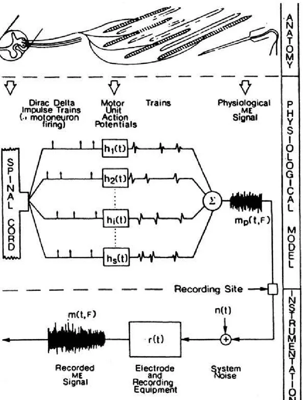
More precisely, MUAP values depend also on the force F generated by the muscle: u = u(t; F ). The value of the EMG signal m(t; F ) sensed at time t depends on the generated force F as well, and is given by the sum of all the MUAPTs uunit(t) generated

by the probed motor units:

m(t; F ) = X

unit∈U

uunit(t; F ) (2.5)

where U is the set of the probed motor units. A comprehensive scheme following the potential from the AP to the recorded EMG signal is shown in Figure 2.2.

In both invasive and surface electromyography, the observed MUAP waveform de-pends on the relative position between the electrode and the active muscle fibers. This relative position may not be constant over time. The MUAP waveform and the EMG signal are also affected by any significant biochemical change in the muscle tissue: this is the case of muscle fatigue, which is a known source of variability for the EMG signal.

Figure 2.2: Scheme of the potential from Activation Potential (AP) to the recorded EMG signal. Image from [19].

2.2

sEMG-based gesture recognition

sEMG-based gesture recognition is a promising technique for the development of Human-Machine Interfaces (HMIs). On the one hand, sEMG has the virtue of being non-invasive, which is essential for many HMIs. On the other hand, entrusting recognition, i.e. signal classification, to automated learning is a successful method for circumventing the complexity of the task by removing the need of a complete physiological understanding of the underlying motor functions.

Automated learning has produced advances with a rich variety of approaches. Whereas the central goal of gesture recognition is signal classification, many other machine learn-ing techniques have been successfully exploited as auxiliary tasks to assist classification at either training or evaluation time, increasing classification accuracy. Examples of auxiliary tasks (detailed in the following subsections) are force estimation by means of regression, and semi-supervised and unsupervised methods for calibration.

However, classical machine learning still requires field-specific knowledge, such as tested and established feature extracting procedures to maximize discriminative power, recourse to the suitable signal domain (time domain, frequency domain, or time-frequency domain), and empirical expertise about the portability of preprocessing and extraction procedures across datasets acquired with different experimental setups.

This need for field-specific knowledge can be overcome by migrating to deep learning algorithms, capable of autonomous feature learning, i.e. to learn good feature represen-tations autonomously, provided sufficient data. The success of deep-learning models has even driven the ambition of reversing the perspective: once trained a satisfactory deep classifier, model explainability can be leveraged to shed light a posteriori on the feature representations, or even on the physiological understanding, lacked a priori. Steps toward demonstrating the feasibility of this approach have already been moved in the related field of electroencephalogram (EEG)-based gesture recognition for Brain-Computer Inter-faces (BCIs): for instance, Nurse et al. in [20, 21], have shown correspondences between channel-time domain filters learned by the first layer of CNNs and known activation patterns of brain regions.

2.2.1

Classical Machine Learning approach

Classical Machine Learning (classical ML), also referred to as traditional or conventional machine learning, is the broad class of non-deep algorithms which includes k-Nearest Neighbors (kNN), Support Vector Machine (SVM), Linear Discriminant Analysis (LDA), and Random Forests (RF) (all with the related kernel methods), and Multi-Layer Percep-tron (MLP) with one hidden layer. In the framework of sEMG-based gesture recognition based on classical ML, the pipeline typically consists of data acquisition, data prepro-cessing, feature extraction, feature selection, model definition, and inference [9, 6].

However, a major disadvantage of the classical ML pipeline is the strong reliance on domain-specific knowledge, needed for feature extraction, feature selection and parameter tuning. The reason why deep learning is appealing for sEMG-based gesture recognition is that it loosens these requirements, replacing feature extraction with feature learning incorporated in the algorithm training.

The general problem of finding good discriminative hand-crafted features is so hard that the quest for better ways to capture the temporal and frequency information of the signal has characterized decades of research. A clear overview of the typical sEMG features identified and used can be found in [6], and can be summarized by domain as follows:

• time domain: Root Mean Square (RMS), variance, Mean Absolute Value (MAV), Zero Crossings (ZC), Slope Sign Changes (SSC), waveform length, histogram; • frequency domain: Short Time Fourier Transform (STFT), cepstral coefficients; • time-frequency domain: Marginal Discrete Wavelet Transform (MDWT).

Two significant studies on sEMG classification with traditional ML techniques were made by Hugdings in [22] and Englehart and Hudgins [23], who studied the classification problem of 4 hand gestures and obtained a classification accuracy higher than 90% by working with 200 ms segments of 4 channel sEMG signals, extracting 5 time-domain features and feeding them to MLP and LDA classifiers, robustifying the assignment by applying a majority vote window to the predictions. Instead, Castellini et al. [53] worked on 3 types of grasp motions and achieved a 97.1% classification accuracy using the RMS value from 7 electrodes as the input to an SVM classifier.

The first successes in the classification of a large number of hand gestures were ob-tained by Kuzborskij et al. [25], using any of the proposed features in both time- and frequency-domain, fed to a SVM classifier with Radial Basis Function (RBF) kernel, and reaching a 70-80% accuracy on the 52 hand gestures of the 8-channel database Non-Invasive Advanced Prosthetics (NinaPro) presented by Atzori et al. in [26]. These results where improved by Atzori et al. [27], by considering linear combination of features and using a RF classifier resulting in an average accuracy of 75.32%; and further improved by Gijsberts et al. in [28], by evaluating different kernel classifiers jointly on EMG and acceleration signals, increasing classification accuracy by 5%.

2.2.2

Deep Learning Revolution

In recent years, sEMG-based gesture recognition has seen a progressive shift from tra-ditional machine learning to deep learning. Deep Learning (DL) is the class of machine learning algorithms that differ from classical ML approaches in that feature extraction is part of the model definition, therefore obviating the need for hand-crafted features.

Existing deep learning architectures are mainly based on two kinds of architecture: the Convolutional Neural Network (CNN), successfully deployed for image classification due to its ability to capture spatial (but also temporal) information of the signal, and Recurrent Neural Network, which allows to exploit the sequential nature of the data and has had successes in speech recognition. The work of this master thesis is exclusively fo-cused on the CNN architecture. Although deep algorithms themselves are not new, they are the most computationally demanding, so that deep classifiers gained attention only relatively recently, thanks to increased availability of data and powerful improvements in computing hardware [29].

The advantage of deep architectures is their ability to incorporate feature learning: a consistent part of the traditional pipeline can be entrusted to the training of the algorithm, which has enough capacity to learn good feature representations on its own. This mitigates the reliance on rigid combinations of preprocessing steps and precise sets of hopefully discriminative features.

The first end-to-end DL architecture was proposed by Park and Lee [11], who built a CNN-based model for the classification of six common hand movements resulting in a better classification accuracy compared to SVM. Atzori et al. [10] proposed a simple CNN

architecture based on 5 blocks of convolutional and pooling layers to classify the 52 hand gestures from the NinaPro database [26], reaching classification accuracy comparable to those obtained with classical methods, though not higher than the best performance achieved on the same problem using a RF classifier.

Geng et al. [12] and Wei et al. [30] improved the results across various datasets by adding batch normalization and dropout (layer types explained in Subsections 3.3.1 and 3.3.3, respectively) to the model architecture, and by using a high-density electrode array, thus benefiting from the setup of High Density sEMG (HD-sEMG). Building the analysis on instantaneous EMG images [12] achieves a 89.3% accuracy on a set of 8 movements, going up to 99.0% when using majority voting over 40 ms signal windows. In [30] it is shown that for some movements a significant role is played by a small, group of muscles, and therefore a multi-stream CNN architecture is used that divides the inputs into smaller images, to be separately processed by convolutional layers before being merged with fully connected layers, reporting a increase in accuracy by 7.2% (from 77.8% to 85%).

Successful approaches also involve multi-modality data (also called sensor fusion): Du et al. [14] exploit the auxiliary information of a data glove to add semi-supervised auxiliary tasks (regression on glove signals) to a CNN, reporting improved classification accuracy.

2.2.3

State-of-the-art on the variability factors

Currently, the state-of-the-art of sEMG-based gesture recognition is coping with chal-lenging issues. The sEMG signal is severely affected by many variability factors such as differences between subjects, fatigue, user adaptation and the variability introduced from the re-positioning the electrodes at each session of data collection. These issues limit long-term use and temporal reliability of the devices relying on sEMG analysis.

In the framework of machine learning, these factors of variability can be modeled with the concept of data sources, i.e. data subsets coming from different distributions (the concept of multi-source data is defined in Subsection 4.1.3). The Multi-source nature of the data makes machine learning on EMG data a challenging problem, where the ambition is to improve the inter-source generalization capability of classifiers. Examples of this are the inter-posture, inter-session and inter-subject scenarios. Up to know, for

instance, the performance with Leave-One-Subject-Out cross-validation (LOSOCV) is still much lower than that reached with Within-Subject cross-validation (WSCV) on the main public benchmark databases [8].

Some studies have already dealt with inter-subject variability, resorting to recalibra-tion techniques or model adaptarecalibra-tion methods often moving from the technique of batch normalization (explained in Subsection 3.3.1). The network proposed in [31] takes as in-put downsampled spectrograms (i.e. time-frequency representations) of sEMG segments, and improvement is achieved by updating the network weights using the predictions of previous sessions corrected by majority voting. In [8] it is assumed that, while the weights of each layer of the network learn information useful for gesture discrimination, the mean and variance of the batch normalization layers store information related to discrimination between sessions/subjects. Moreover, a variation of batch normalization called Adaptive Batch Normalization (AdaBN) is used in [32]: only the normalization statistics are updated for each subject using a few unlabeled data, improving performance with respect to a model without adaptation.

In [33] transfer learning techniques are used to exploit inter-subject data learned by a pre-trained source network. In this architecture, for each subject a new network is instantiated with weighted connections to the source network, and predictions for a new subject are based both on previously learned information and subject-specific data. Doing so achieves an accuracy of 98.3% on 7 movements.

2.2.4

State-of-the-art on the Unibo-INAIL dataset

The state-of-the-art of sEMG-based hand gesture recognition on the Unibo-INAIL dataset is exposed by Milosevic et al. in [15]. The dataset itself represents the state of the art with regard to databases able to explore inter-subject, temporal, and postural variability, and is extensively described in Section 4.1.

Knowledge about the performance of classifiers on the dataset is limited to classical machine learning classifiers, namely Support Vector Machine (SVM), Neural Network (NN) with only one hidden layer, Random Forest (RF) and Linear Discriminant Analysis (LDA). However, these classifiers have been used to explore a large number of data partitions and training strategies, trying to optimize the generalization capability on new arm postures and new days.

The evaluated algorithms have similar recognition performance, higher than 90% (precise values depending on data partition and training strategy). The Radial Basis Function (RBF)-kernel SVM is at present the one achieving the highest accuracy, both intra-session and inter-session.

With regard to inter-session generalization, the baseline classification accuracy was higher than 90% for intra-posture and inter-day analysis, suffering a degradation of up to 20% when testing on data from different postures or days. This is consistent with the inter-session accuracy decline shown for other datasets (e.g. the 27% morning-to-afternoon decline reported for the NinaPro Database 6 by Palermo et al. [34]). The work showed that this inter-posture and inter-day accuracy decline is mitigated by training with combinations of data from multiple sessions. Moreover, results on temporal vari-ability show a progressive user adaptation trend and indicate that (re)training strategies should prioritize the availability of recent data.

However, despite the variety of strategies and the number of results, the state of the art has two limitations. The first limitation is that, as said above, the state of the art on this dataset is limited to classical machine learning algorithms. The second limitation concerns data preprocessing: all the algorithms are applied on singled out, instantaneous signal values (i.e. 4-dimensional data points whose only dimension is channel number), so that the sequential nature of the EMG signal is not exploited at all. This master thesis addresses both these limitations.

Chapter 3

Deep Learning and Convolutional

Neural Networks

Deep learning is the sub-field of machine learning which deals with deep neural networks, i.e. neural networks having more than one hidden layer. Deep learning is currently the fundamental approach for the development of artificial intelligence. One of the most important deep neural network architectures is the convolutional neural network, which is the model used in this work.

This chapter is structured as follows:

◦ Section 3.1 introduces neural networks and deep learning, contextualizing them with respect to machine learning and artificial intelligence;

◦ Section 3.2 provides the fundamentals of deep networks training, and illustrates some specific techniques and settings used in this work;

◦ Section 3.3 introduces convolutional neural networks, explaining the essential layer types (i.e. convolutional and fully connected) and also introducing the other par-ticular layers used in this work.

3.1

Neural Networks and Deep Learning

Deep learning (DL) is the branch of Machine Learning (ML) which is nowadays the base of the research and applications of Artificial Intelligence (AI) [35], and in the last decade

has produced vast advances in many fields such as speech recognition [36] and image recognition [37], cancer detection [38], self-driving vehicles [39], and playing complex games [40]. In some applications, DL models already exceed human performance.

The superior performance of DL models resides in the ability to incorporate au-tomated data-driven feature extraction selection, i.e. the ability to extract high-level features from raw data by using statistical learning on large datasets. This approach produces effective representations of the inputs space, based on powerful discriminative features, in a different way from the earlier approaches based on non-deep ML, which are built on hand-crafted features or rules designed by expert researchers.

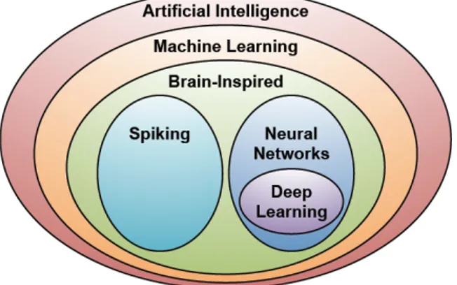
It is important to contextualize clearly the relationship DL has with AI and ML, as illustrated in Figure 3.1. With respect to the broad domain of AI, ML can be considered a vast sub-domain. Inside ML, is the area referred to as brain-inspired computation, whose interest is the developing of programs or algorithms whose basic functionality is inspired by natural brains and aims to emulate some aspects of how we currently understand the brain works [41]. Brain-inspired computing is divided into to main branches: spiking computing and DL. Spiking computing, which is beyond the scope of this work, takes inspiration from the fact that communication between neurons happens via spike-like pulses, with information not simply coded in spike’s amplitude, but also in the timing of the spikes. In contrast, the branch of brain-inspired computing relevant here is Neural Networks (NNs), which are a well-known ML algorithm.

Figure 3.1: Deep Learning contextualized with respect to Artificial Intelligence and Machine Learning. Image from [41].

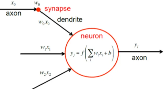
neuron can be modeled as a weighted sum of the input activations, followed by a non-linear function with threshold and bias, which generates the neuron’s output signal [42] as illustrated in Figure 3.2. By analogy, neural networks are built assembling units (also referred to as neurons) which apply a non-linear function to the weighted sum of the input values they receive.

Figure 3.2: Model of the computations performed by a brain neuron: xi are the input

activations, wi are the weights of the weighted sum, f (·) is the non-linear function, and b is the

bias term. Image from [42].

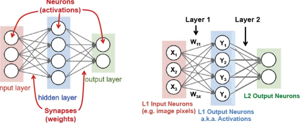
Neural Networks, like the computations they execute, are structured as layers of units, and an example scheme is shown in Figure 3.3. The neurons belonging to the input layer receive the raw input values, and propagate them to the neurons of the middle layer, called the hidden layer. The weighted sums computed by one or more hidden layers ultimately reach the output layer, whose units compute the final output of the network. Taking the brain-inspired terminology further, the neuron outputs are referred to as activations, and the weights are sometimes called synapses. In addition to the network structure, Figure 3.3 also shows the computations made at each layer, which follow the formula yj = f 3 X i=1 Wijxi+ b ! = (3.1) = f (Wx + bj) , (3.2)

where x are the input activations, W are the weights, bj are the bias terms, yj are the

Figure 3.3: Scheme of a simple neural network’s structure and terminology. Left: neurons and synapses. Right: weighted sum computation for each layer (bias term b omitted for simplicity).

Image from [41].

Deep learning is the field of Neural Networks which focuses on Deep Neural Networks (DNNs), which are networks having more than one hidden layer, or, equivalently, more than three layers in total (typically, from five to more than a thousand [41]). DNNs have the ability to learn high-level features with more complexity and abstraction than shallow (i.e. non-deep) neural networks. For instance, in image processing, pixels of an image are fed to the first layer of a DNN, whose outputs can be interpreted as representing the presence of low-level features in the image, such as lines and edges. Subsequent layers progressively combine these features, eventually yielding a measure associated to the presence of higher level features (e.g. edges are combined into shapes, then into sets of shapes). As final output, the network produces an estimate of the probability that the highest-level features comprise a particular object or scene. This paradigm is referred to as deep feature hierarchy, and is what gives the DNNs the ability to obtain superior performance.

3.2

Training deep networks: gradient descent and

back-propagation

In a DNN, like in machine learning algorithms in general, there is a basic program that does not change while learning to a desired task. For DNNs, the basic program is the structure of the functions implemented by the layers, and learning consists in

determining the value of the network’s weights and biases, through an optimization called training. Once trained, the network can execute its task by computing the output using the optimized weights and biases. Running the trained networks to evaluate inputs is referred to as inference.

The training scenario relevant in this work is the supervised training for a classi-fication task. In classiclassi-fication tasks, trained DNNs receive input data (e.g. the pixels of an image) and return vector of scores, one for each class. The highest-score class is the one the network estimates as most probable. The main goal of DNN training is to optimize the weights and the bias values so as to maximize the score of the correct class and minimize the scores of the incorrect classes. In supervised learning, the correct class of the data the network is trained on is known. The dissimilarity between the ideal correct scores and the scores computed by the DNN (based on its current weights and biases) is called the loss L, which is the objective function of the training, i.e. function to minimize.

A widely used algorithm for weight optimization is a hill-climbing iterative opti-mization procedure called gradient descent. In gradient descent, at each iteration t the weights wij is updated by subtracting a multiple of the gradient of L with respect to the

weights. Element-wise:

w_ij(t+1)= w_ij(t)− α ∂L ∂wij

(3.3)

where the multiplication factor α is called learning rate. Iterating reduces L.

In contrast with weights and biases, which are referred to as model parameters since they are the arguments of the objective function to minimize, the learning rate α is not involved in differentiation and hence is a training hyper-parameter, i.e. a constant that regulates the optimization without being affected by training. As the hyper-parameters describing the structure or training of any machine learning model, α can be tuned to the optimal value through cross-validation (which can be computationally expensive) or through a shorter preliminary analysis (as done in this work), with a further speed-up commonly yielded by following heuristics instead of grid search. The optimal α is typically small (some orders of magnitude below unity), but the its order of magnitude is strongly dependent on data, task, and model architecture. Hence the search must cover different orders of magnitude.

Finer techniques for tuning the learning rate are scheduling and recourse to per-parameter learning rates. (1) With scheduling, α is reduced over the iterations, typically with a stepwise or exponential decay, in order to adapt the tuning to different moments of the gradient descent. (2) On the other hand, introducing per-parameter learning rates allows to perform a customized tuning on different parameters or groups of parameters. Both techniques come at the cost of an increased number of combination to explore.

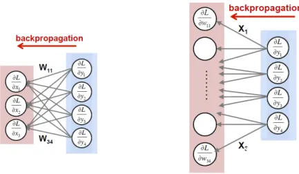
An efficient procedure for computing the partial derivatives of the loss is back-propagation, which derives from the chain rule of calculus and operates by passing values backwards through the network to compute how the loss is affected by each weight. Com-putation using back-propagation, illustrated in Figure 3.4, requires some steps used also for inference. To back-propagate through each layer, one has to: (1) compute the gradi-ent of L relative to the weights from the layer inputs (i.e., the forward activations) and the gradient of L relative to the layer outputs; (2) compute the gradient of L relative to the layer inputs from the layer weights and the gradients of L relative to the layer outputs. It is worth to note that back-propagation requires intermediate activations to be preserved for the backward computation, so that training has increased storage requirements compared to inference.

Figure 3.4: Example of back-propagation through a neural network: (1) (left) computation of the gradient of the loss relative to the layer inputs; (2) (right) computation of the gradient

of the loss relative to the weights. Image from [41].

Another popular training method, orthogonal to the techniques exposed so on, is fine-tuning. In fine tuning, the weights of a trained network are available, and are used as a

starting point for the iterative optimization. This practice results in faster training than using random initialization. Moreover, the scenario in which the weights are adjusted for a new dataset is the sub-field of machine learning defined transfer learning.

More specific training settings and techniques used in this work are explained in the next subsections.

3.2.1

Cross-entropy loss

When training neural networks, a convenient choice for the objective function (adopted also in this work) is the cross-entropy function. Originating in the field of probability theory and information theory, the main virtue of cross-entropy is that it leverages the soft assignments produced by the network, interpreting them as probabilities. Given a multiclass classification task on C classes, the loss for the observation xi is computed by

summing the losses due to each soft assignment ˆyic with respect to the true label yic (i.e.

the one-hot encoding):

loss(xi) = − C

X

c=1

yiclog ˆyic, (3.4)

with arbitrary choice for the base; e.g., taking the logarithm in base 2 yields a result in bits, whereas choosing base e yields a result in nats. The overall loss L is then computed by averaging over all the items to classify. When working with an unbalanced dataset, it can be useful to weight the elements by class when taking the average.

3.2.2

Stochastic gradient descent with mini-batches

Stochastic Gradient Descent (SGD) is a variation of gradient descent which helps avoiding local minima during training. This technique does so introducing randomness in the optimization process by randomly partitioning the training set, referred to as the batch, into B equal-sized subsets called mini-batches. Then, gradient descent is performed using a single mini-batch per iteration, cycling over all the mini-batches. The sequence of B iterations that processes all the mini-batches exactly once is referred to as an epoch. Thus, during an epoch, all the data contribute to the optimization to the same amount. At the end of each epoch, the split into mini-batches is re-randomized, in order to prevent

systematic bias generated by a particular order of comparison of the data.

It is important to note that the avoidance of local minima provided by SGD comes at the cost of introducing a new training hyper-parameter, the batch size b (or, equivalently, the number of batches B).

Since some sources reserve the name SGD for the extreme case b = 1, in the remainder of this work the term SGD with mini-batches will be used to avoid confusion.

3.2.3

L

regularization

The technique of L2 regularization takes its name from the L2-norm and is a method to

counter overfitting. It consists in adding to the loss a multiple of the squared L2-norm of

the vector of all the parameters, and using the new formula Lreg as objective function.

In formulas, for a deep neural network:

Lreg= L0+ LL2 = (3.5) = L0+ λL2 Nlayers X l=2 nl−1 X i=1 nl X j=1 |w(l)_ij |2, (3.6)

where L0 is the non-regularized loss, LL2 is the regularization term, Nlayers is the number of layers, nlis the number of neurons in layer l, and w(l)ij is the weight connecting neuron

i of layer l − 1 to neuron j of layer l. The factor λL2 is the training hyper-parameter regulating the amount of regularization enforced. Too low λL2 has no effect, and too high λL2 incurs underfitting. The optimal value can be determined via preliminary analysis or cross-validation, covering different orders of magnitude.

3.3

Convolutional Neural Networks

Deep networks have a vast variety of architectures and sizes, continuously evolving to increase performance. Convolutional neural networks are a successful class of architec-tures, which can be introduced only after surveying the strategies used to progressively reduce the storage and computation required by layers: sparsity, structured sparsity, weight sharing, and convolution.

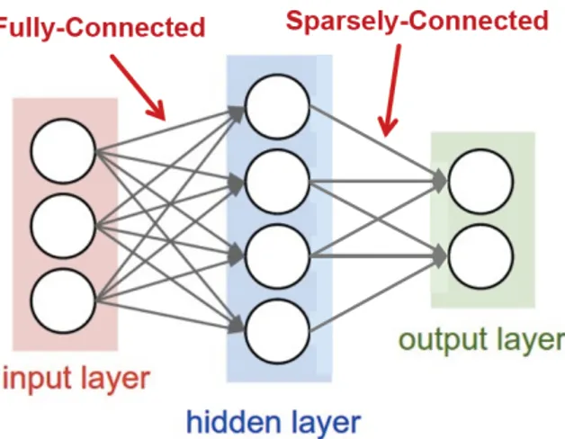
Figure 3.5, and in this case they are defined Multi-Layer Perceptrons (MLP). In a FC layer, all outputs units are connected to all inputs units, so that all output activations are computed with a weighted sum of all input activations. Although the FC configuration requires significant computation and storage, in many situations it is possible to zero some weights (thus removing the relative connections) without impacting performance. The resulting layer, also shown in Figure 3.5, is called sparsely connected layer.

Opposed to generic sparsity, structured sparsity is the configuration in which each output is only a function of a fixed-size window of inputs. Even further efficiency is gained when the computation of every output employs the same set of weights. This configuration is known as weight sharing, and strongly reduces the storage requirements for weights. A particular case of weight sharing arises when the computation is structured as a convolution, as shown in Figure 3.6: the weighted sum for each output activation is computed using only a narrow neighborhood of input activations (by zeroing the weights outside the neighborhood), and every output shares the same set of weights (i.e., the filter is space invariant). This gives rise to convolutional (CONV) layers, which are the characteristic building block of convolutional neural networks.

Figure 3.6: 2d convolution in traditional image processing. Image from [41].

Convolutional Neural Networks (CNNs) are a successful deep network architecture, composed of multiple CONV layers, as shown in Figure 3.7. In CNNs, each layer gener-ates a progressively higher-level representation of the input data, referred to as feature map (fmap), extracting the essential information for the network’s task. Modern CNNs have attained superior performance by implementing a very deep hierarchy of layers. CNN are widely used in a variety of applications including image understanding [37], speech recognition [43], robotics [44] and game play [40]. In this work, CNNs are applied to the task of classifying time windows of a 4-channel signal.

CNNs fall into the category of feed-forward networks. In a feed-forward network, all computations are executed as a sequence of operations taking place from one layer to the next one. A feed-forward network has therefore no memory, and the output for a given input is always identical irrespective of the history of the inputs fed previously.

Each CONV layer is mainly constituted by high-dimensional convolutions, as shown in Figure 3.8. In this computation, the input activations of a layer have the structure of a set of 2d input feature maps (ifmaps), each referred to as a channel. Each channel is convolved with a distinct 2d filter from the stack of filters, one for each channel. The stack of 2d filters being a 3d structure, it is sometimes collectively called a 3d filter. The results of the convolutions at each point are summed across channels, and a 1d bias is optionally [45] added to the results. The result of this computation are the output activations constituting one channel of the output feature map (ofmap). Additional output channels can be created by applying additional 3d filters on the same input.

With the notation for shape parameters defined in Table 3.1, the computation exe-cuted by a CONV layer is described by the formula

O[z][u][x][y] = B[u] + C−1 X k=0 S−1 X i=0 R−1 X j=0

I[z][k][U x + i][U y + j] ∗ W[u][k][i][j], (3.7)

with 0 ≤ z < N, 0 ≤ u < M, 0 ≤ x < F, 0 ≤ y < E, (3.8) E = H − R + U U , F = W − S + U U , (3.9)

where O, I, W and B are the matrices of ofmaps, ifmaps, filters and biases, respectively, U is a fixed stride size, and ∗ denotes discrete convolution. A graphical representation of this computation is shown in Figure 4.2 (where biases are omitted for simplicity).

To align the CNN terminology with the general DNN terminology, is it worth re-marking that

• filters are composed of weights (corresponding to synapses in nature);

• input and output feature maps (ifmaps, ofmaps) are composed of activations of inputs and output neurons.

Figure 3.8: High-dimensional convolutions in CNNs. Image from [41].

Shape parameter Meaning

N batch-size of 3d maps

M number of 3d filters / number of batch channels

C number of ifmap/filter channels

H/W ifmap plane heigth/width

R/S filter plane heigth/width (= H or W in FC)

E/F ofmap plane heigth/width (= 1 in FC)

Table 3.1: Shape parameters of a CONV/FC layer.

In the CNN used in this work, the CONV layers are CONV-1d layers, i.e. layers performing a 1-dimensional convolution. Though less common, CONV-1d layers follow the same principles as CONV-2d layers, but work with inputs having 1 dimension (plus channel number). The choice to use CONV-1d layers was made in order to act on the time dimension of the signal, while using the 4 sEMG channels as CNN input channels. In addition to CONV layers and FC layers, the CNN implemented in this work con-tains other elements, namely the rectified linear unit, batch normalization and dropout,

whose mechanisms are explained in the following two subsections. These three kinds of intervention on activations are sometimes conceptualized as layers.

3.3.1

Batch-normalization

Controlling the input distribution across layers can speed up training and improve accu-racy. Accordingly, the distribution of a layer’s input activations (described by its mean µ and standard deviation σ) can be standardized to zero mean and unit standard deviation. Batch Normalization (BN) [46] is the technique in which the standardized activations are further scaled and shifted, undergoing the transformation

y = √x − µ

σ2_{+ ε}γ + β, (3.10)

where the parameters γ and β are learned from training, and ε is a small constant used to avoid numerical problems. Batch normalization is mostly applied between the CONV or FC layer and the non-linear activation function, and is usually turned off after training.

3.3.2

ReLU activation function

Non-linear activation functions are typically applied after each CONV or FC layer. The most common functions used to introduce non-linearity into a DNN are shown in Figure 3.9. Historically, the sigmoid and the hyperbolic tangent are the most conventional, while the Rectified Linear Unit (ReLU) has become common in the last years due to its simplicity and its ability to make training faster [47]. The leaky ReLU, parametric ReLU, and exponential LU are variations of the ReLU explored for increased accuracy. ReLU is mostly applied after the CONV or FC layer or after batch normalization (if present).

Figure 3.9: The most common non-linear activation functions. Image from [48].

3.3.3

Dropout

Dropout is a technique to improve accuracy by reducing overfitting [49, 50]. It works by randomly dropping units (and their connections) from the network during training. This prevents the phenomenon of units co-adaptation, forcing each neuron to learn a feature helpful for computing the correct output. In particular, the random dropout of the units of the interested layer during training is regulated by the drop probability p, for which a common value is p = 0.5. On every forward pass, each unit is zeroed out independently and randomly, drawing from the Bernoulli distribution parameterized by p. Moreover, the outputs are multiplied by _1−p1 . Dropout is active only during training: during inference, the dropout layer is disabled (or, equivalently, the drop probability p is set to 0). Dropout is mostly applied immediately before the CONV or FC layer.

Chapter 4

Materials and Methods

This chapter explains all the materials and methods used in this master thesis. It is structured as follows:

◦ Section 4.1 exhaustively describes the Unibo-INAIL dataset;

◦ Section 4.2 details the implemented machine learning pipeline, preprocessing, CNN architecture and training settings;

◦ Section 4.3 defines the concept, essential in this work, of training strategy based on training set composition, and illustrates the training strategies used.

4.1

Unibo-INAIL dataset

The work of this master thesis is entirely focused on the Unibo-INAIL dataset. The Unibo-INAIL dataset is a surface electromyography (sEMG) dataset realized to explore the impact of arm posture and temporal variability (either alone or combined) on sEMG-based hand gesture recognition. The dataset was presented by Milosevic et al. in [15], and was built on the preliminary analysis carried out by Benatti et al. in [51]. This master thesis evaluates the performance of Convolutional Neural Networks (CNNs) trained on the dataset with all the training strategies described in [15], where the performance of classical machine learning algorithms is reported.

The data were acquired from 7 able-bodied (i.e. non-amputee) subjects performing 6 discrete hand gestures in 4 arm postures, repeated for 8 days, thus probing a total

of 224 different data sources, each identified by three discrete indexes (subject, day and arm posture) and containing 6 classes, i.e. five hand gestures plus the rest position. This acquisition protocol, in addition to investigating the signal patterns associated to the 6 classes, allows to characterize the following sources of variability affecting signal and patterns:

• inter-posture variability: for each subject individually, keeping sensors on, different arm postures and wrist orientations cause variability in signal and patterns, due to differences in muscle activity and muscle position (since sensors are only fixed with respect to the skin);

• inter-day variability: for each subject individually, temporal variability of signal and patterns are mainly due to two factors:

– sensor placement: from day to day, the sensors are removed and repositioned, causing differences in signal and patterns, due to the change of the relative position of the electrodes with respect to the muscles;

– user adaptation: user adaptation (explained in Subsection 4.1.4) is the tran-sient observed when the inter-day differences in gesture execution decrease over time, due to the fact that new users adapt to the repetitive exercise during the first days;

• inter-subject variability: signal and patterns are influenced by the anatomical vari-ability between subjects (even if all able-bodied).

For the research on sEMG-based hand gesture recognition for reliable Human-Machine Interfaces (HMIs), the Unibo-INAIL dataset is a valuable ground for two reasons. The first reason is that the acquisition setup is based on commercial sensors, chosen so as to make the setup is easily repeatable and thus suitable for integrated HMI controllers [52]. The second reason is that the Unibo-INAIL dataset is the first public sEMG dataset to date to include both arm-postural and session variability, providing a realistic scenario for evaluating classification algorithms and training approaches.

4.1.1

Unibo-INAIL collaboration and motivation for the dataset

The Unibo-INAIL dataset is the results of a research project funded by the Istituto Nazionale per l’Assicurazione contro gli Infortuni sul Lavoro (INAIL), in which the Uni-versity of Bologna (Unibo) was designated for assessing the feasibility of real-time control of poly-articulated hand prostheses by means of pattern recognition algorithms imple-mented on a microcontroller. The project was inspired by a previous study by Castellini et al. [53] on intuitive prosthesis control, which demonstrated that SVMs can recognize different muscle activation patterns with high precision. In particular, the SVMs classify gestures up to a precision of 95% and approximate the forces with an error of as little as 7% of the signal range, sample-by-sample at 25 Hz.

The first part of the project aimed to assess how accurate the recognition can be on diverse data produced in different conditions (i.e. intra-session scenario), and to verify whether the system was stable on different sessions (i.e. inter-session generalization). Although in prosthetics sensor (re)positioning is less relevant, since sensors are fixed to the prosthesis and thus much less mobile, this variability factor was included, planning future developments.

The second branch of the project involved the validation of the algorithms in real-time control scenario. The controller was implemented on a microcontroller, in a system in which the real-time, fresh data were acquired with the same embedded setup used for the first part of the project, in order to reproduce the previous system. The algo-rithm implementation was also made identical by using the open source machine learning library LIBSVM, which is implemented for both Matlab and C [54].

This master thesis continues the first part of the project, aiming to expand the results obtained for classical machine learning algorithms (SVM, shallow NN, RF and LDA) applied on instantaneous 4-channel signal values. This work extends the analysis to deep CNNs applied on 150 ms time windows of the 4-channel signal.

4.1.2

Outline of acquisition setup and experimental protocol

The acquisition setup, shown in Figure 4.1, was designed to be reliable and repeatable, with characteristics typical of prosthetic applications. However, since all the data are collected from able-bodied (i.e. non-amputee) subjects, the dataset is useful for any HMI application.

The acquisition setup is based on the Ottobock 13E200 pre-amplified single-ended sEMG electrode (Figure 4.2a), which is a commercial sensor. It amplifies and integrates the raw EMG signal to reach an output span of 0 − 3.3V. The sensors have bandwidth spanning 90 − 450Hz and integrate an analog notch filter to remove the noise due to Power Line Interference (PLI), i.e. the capacitive coupling between the subject and the surrounding electrical devices and power grid (detailed in Section 2.1). The output analog signals were acquired with a custom embedded board based on a microcontroller equipped with an internal 16-bit ADC. The digitalized signals were streamed via Bluetooth to a laptop, for storage and off-line data analysis.

The subjects involved were able-bodied (i.e. non amputee) males, 29.5 ± 12.2 years. During the acquisition the subjects worn an elastic armband with 4 Ottobock sensors placed on the forearm muscles involved in the selected movements (i.e. extensor carpi ulnaris, extensor communis digitorum, flexor carpi radialis and flexor carpi ulnaris) as shown in Figure 4.2b. Sensors were placed on the proximal third at 30 mm respectively on the left and on the right side of two axial lines ideally traced on the forearm. Each acquisition consisted in 10 repetitions of each hand gesture, with 3 second contractions interleaved by 3 seconds of muscular relaxation to be later labeled as rest gesture. After each acquisition, gesture segmentation was performed with a combination of manual inspection and an adaptive threshold to separate contractions from rest.

(a) Ottobock sensor used to produce the Unibo-INAIL dataset. Image from [51].

(b) Forearm muscle cross-section and sensors placement. Image from [15].

Figure 4.2

4.1.3

Multi-source data structure

The fundamental property of the Unibo-INAIL dataset is that it contains 224 different data sources, since the data were collected for all the combinations obtained from 7 seven subjects, 8 days and 4 arm postures. Each subject-day-arm posture combination contains all hand gestures (i.e. the classes), each one repeated 10 times. The dataset can thus be regarded as a collection of 224 autonomous sub-datasets, for which the pattern to learn in order to assign signals to hand gestures is subjected to inter-subject, inter-day and inter-posture variability.

In machine learning, data having this structure are defined multi-source data. For the Unibo-INAIL dataset, each combination identified by a 3-ple subject-day-arm posture combination is a source:

source = (u, d, p) with          u = 1, · · · , 7 d = 1, · · · , 8 p = 1, · · · , 4 (4.1)

totalling 224 sources. Each source can be regarded as a smaller, complete dataset con-taining 10 repetitions of all the 6 gestures.

has in statistical learning [7], where it refers to data-subsets having different but similar distributions. The intended meaning is not data coming from different types of sensors or modalities.

The subject-index u refers to the 7 subjects involved. Each one underwent data collection over 8 days: this is the day-index d of the data sources. Arm posture p is the third index, and the four collected arm postures are:

P1. proximal: the only one with the arm not fully extended, and the most common in EMG-based hand gesture recognition literature;

P2. distal;

P3. distal with the palm oriented down: the different wrist orientation aims to introduce additional difference compared to P2 and P4;

P4. distal with the arm lifted up by 45◦. These arm postures are displayed in Figure 4.3.

To constitute the classes of the dataset, five common hand gestures used in daily life were chosen: power grip, two-fingers pinch grip, three-fingers pinch grip, pointing index and open hand. Rest position, recorded when muscles were relaxed between two subsequent movement repetitions, was also included as a class, totalling 6 classes:

G0: rest position: including this class means addressing also the task of gesture

detec-tion, in addition to gesture recognition; G1: power grip;

G2: two-fingers pinch grip;

G3: three-fingers pinch grip;

G4: pointing index;

G5: open hand.

The five hand gestures G1, · · · , G5 are shown in Figure 4.2, together with examples of

4-channel sEMG signal patterns of the gestures and the rest position G0.

NOTE. It is of crucial importance, when handling the Unibo-INAIL dataset, not to mistake arm posture and hand gesture, since they are partitions acting at two different levels: the arm posture is the position of the arm in which all hand gestures (plus rest

position) were executed. Each combination of subject, day and arm posture contains 10 repetitions of all the five hand gestures plus rest, and can thus be regarded as a complete sub-dataset containing all the 6 classes.

Figure 4.3: Arm postures of the Unibo-INAIL datase. P1: proximal; P2: distal; P3: distal with the palm oriented down; P4: distal with the arm lifted up by 45◦. Image from [51].

4.1.4

User adaptation

User adaptation is the source of temporal variability which consists in a transient ob-served in the first days of many benchmarks datasets for sEMG-based hand gesture recognition [55, 56, 57]. The phenomenon consists in the fact that the inter-day differ-ences in gesture execution decrease over time, due to the tendency of users to adapt to the repetitive exercise during the first days.

In literature, these inter-day differences are detected and measured by analysing how classification accuracy deteriorates when passing from intra-day validation to inter-day validation. With this method, classical machine leaning algorithms have already been able to highlight user adaptation also on the Unibo-INAIL dataset [15], which means that user the adaptation transient is not masked by the temporal variability caused by day-to-day sensor repositioning, which affects the signal on both the earlier and later days.

Figure 4.4: Amplified sEMG signal patterns of the hand gestures constituting the classes of the Unibo-INAIL dataset. G0: rest position; G1: power grip; G2: two-fingers pinch grip; G3:

4.2

Pipeline and CNN architecture

4.2.1

Preprocessing: windowing

Data preprocessing consisted in an overlapping windowing scheme: the electromyogram signals were decomposed into segments of duration 150 ms, with a 75% overlap between consecutive ones. Since the dataset was acquired with 4 electrodes and sampling rate 500 Hz, for approximately 15 min/session, this windowing produced a sample size of the order of M ∼ 25.000 windows/session, each with dimensions 75 samples × 4 channels. Each window was given the label of the hand gesture of its central sample.

The choice of duration 150 ms and overlap 75% was made with a preliminary analysis exposed in Subsection 6.2.1, showing that duration 150 ms yields a higher classification accuracy than 50 ms and 100 ms.

Window duration and overlap are parameters strictly related to the engineering prob-lem met in HMI development: real-time classification robustness, especially during tran-sients. Longer windows allow to reduce the impact of transients, but the window length must be shorter than 300ms [22] to satisfy real-time usage constraints. 150 ms is a favourable but realistic compromise. With regard to overlap, 75% is a good compromise to produce an adequate sample size (M ∼ 25.000 windows/session) without exceeding in redundancy.

4.2.2

Three-way data partition

Each of the 224 sessions (i.e. combinations of subject, day and arm posture) of the dataset was subjected to a three-way data partition.

Random 10% holdout. First, a random 10% of the signal windows were held out as test set. Reproduction of identical holdout at each execution was ensured by setting NumPy’s pseudorandom seed to a fixed value. No stratification with respect to class was enforced. This test set was used in the very last step of the pipeline, to compute on new data:

• the inter-posture test accuracy of the best postural training strategy; • the inter-day test accuracy of the best multi-day training strategy.