ALMA MATER STUDIORUM UNIVERSIT `
A DI BOLOGNA
SCHOOL OF ENGINEERING: FORL`I CAMPUSMaster Degree in Aerospace Engineering
SECOND CYCLE MASTER’S DEGREE IN INGEGNERIA AEROSPAZIALE/AEROSPACE ENGINEERING Class: LM-20
GRADUATION THESIS IN:
SPACECRAFT ORBITAL DYNAMICS AND CONTROL
Optimising in-flight calibration approach for the magnetometer
experiment on the ESA JUICE mission
Student:
Lorenzo Sanit`a Matricola 0000871869
Academic Supervisor:
Dott. Marco Zannoni
Research Supervisor:
Abstract
In this study the main aim has been to analyse and improve some important aspects of the in-flight calibration process for the three Earth fly-bys planned for the ESA JUICE space mission. In fact it has been developed a calibration script that is capable to correct uncalibrated data from the misallignment and scaling errors towards the expected values of magnetic field from IGRF13 model. Also the experimental process of reproduction of the magnetic field data from JUICE Earth fly-bys prooved the efficiency of the script to control the instrumentation for the gain control during the in-flight calibration. It has also been proved the low influece of the Soft Iron effect on the intrumentation, helping then to reduce the errors associated to misallignments and to the sensors offsets.
Contents
List of Figures 3 1 Introduction 7 1.1 Hosting structure . . . 7 1.2 Objectives . . . 7 1.3 ESA JUICE . . . 8 1.3.1 Mission overview . . . 8 1.3.2 Mission objectives . . . 10 1.3.3 Payoload . . . 111.4 JMAG Calibration overview . . . 12
2 Generation of magnetic field data relative to JUICE Earth fly-bys 15 2.1 JUICE Earth fly-by trajectories . . . 17
2.2 TU Braunschweig Magnetic field data . . . 20
2.3 Python script Magnetic field data . . . 22
2.4 Data comparison . . . 25
3 Cluster data comparison and development of a calibration script 28 3.1 ESA Cluster II mission . . . 28
3.2 Magnetic field data comparison . . . 31
3.3 Calibration script . . . 36
3.4 A particular solution for the Cluster trajectories . . . 39
4 Experimental test for the reproduction of the Earth Magnetic field components for the ESA JUICE Earth fly-bys 43 4.1 Instrumenation used . . . 43
4.2 Experiment results . . . 47
5 JACS coils Ansys simulations 55 5.1 Soft Iron and Hard Iron effect . . . 55
5.3 Simulation results . . . 62 5.4 Computation of the magnetic field for the ferromagnetic materials . 63
6 Conclusions 70
Bibliography 72
List of Figures
1.3.1 Official logo of ESA JUICE . . . 8
1.3.2 ESA JUICE infographic portrait. [Airbus] . . . 9
1.3.3 ESA JUICE Timeline table . . . 10
1.3.4 ESA JUICE representation . . . 12
2.0.1 Main mission events table from JUICE Consolidated Report on Mission Analysis (CReMA). . . 16
2.1.1 First JUICE Earth Fly-by designed for May 31 2023. . . 17
2.1.2 Second JUICE Earth Fly-by designed for September 2 2024. . . 17
2.1.3 Third JUICE Earth Fly-by designed for November 26 2024. . . 18
2.1.4 All the three Earth Fly-bys plotted together around the sphere model. . . 18
2.1.5 A schematic view of the Earth magnetosphere deformed by external contributions. [NASA] . . . 19
2.2.1 JUICE Earth first fly-by magnetic field prediction . . . 20
2.2.2 JUICE Earth second fly-by magnetic field prediction . . . 21
2.2.3 JUICE Earth third fly-by magnetic field prediction . . . 21
2.3.1 JUICE Earth first fly-by magnetic field computed with the Python script. . . 23
2.3.2 JUICE Earth second fly-by magnetic field computed with the Python script. . . 23
2.3.3 JUICE Earth third fly-by magnetic field computed with the Python script. . . 24
2.4.1 Summary of magnetic field data from TU Braunschweig. . . 25
2.4.2 Summary of magnetic field data from Python script. . . 25
2.4.3 Summary of absolute and relative errors between. . . 25
2.4.4 Summary of JUICE Earth fly-by magnetic field data from the two Imperial college students Rebecca Dunkley and Verity Cook. . . . 26
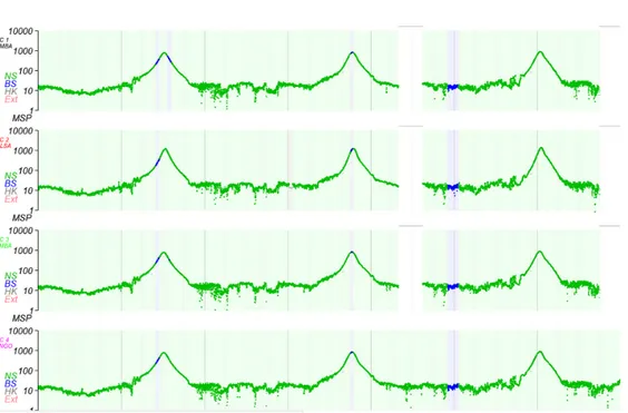
3.2.1 Magnetic field data from all the four spacecraft of Cluster for
dif-ferent dates including the selected time period. . . 31
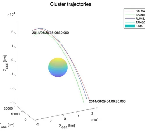
3.2.2 Trajectories of the four Cluster spacecraft during the Earth fly-by of the 28th-29th June 2014. . . 32
3.2.3 Magnetic field components for the first spacecraft SALSA Earth fly-by for the selected time period for both Cluster and Python script. . . 33
3.2.4 Comparison between the modulus of the Cluster data and the Python script data. . . 34
3.2.5 A closer look to the modulus of magnetic field components for the first spacecraft SALSA Earth fly-by for shorter time period for both Cluster and Python script. . . 34
3.3.1 Calibrated magnetic field components for the first spacecraft SALSA Earth fly-by for the selected time period compared with the Python script data. . . 37
3.3.2 Residuals computed between the calibrated Cluster data and the Python script data. . . 37
3.4.1 The anomalous trajectories for the Cluster spacecraft from the data generated with respect to the GSM frame of reference. . . 39
3.4.2 Components of the position of the first Cluster spacecraft for the data generated in GSM. . . 40
4.1.1 The HACM Sensor used for the experiments . . . 44
4.1.2 The HACM sensor fitted inside the MU-metal can. The coil is attached to the internal part of the can. . . 44
4.1.3 Wooden box containing the can in Mu-metal with the cylindrical coil inside. . . 45
4.1.4 Most relevant parameters from Keithley 6221 data sheet. . . 45
4.1.5 The Keithley 6221 used for the experiment. . . 46
4.1.6 The GPIB to USB converter used for the experiment. . . 47
4.2.1 Comparison between the profiles of the computed magnetic field and the experimental data for the first fly-by. . . 48
4.2.2 Comparison between the profiles of the computed magnetic field and the experimental data for the second fly-by. . . 49
4.2.3 Comparison between the profiles of the computed magnetic field and the experimental data for the third fly-by. . . 50
4.2.4 Table with the comparison between the maximum and the mini-mum values of magnetic field for each component of the first fly-by. 51 4.2.5 Table with the comparison between the maximum and the min-imum values of magnetic field for each component of the second fly-by. . . 51
4.2.6 Table with the comparison between the maximum and the mini-mum values of magnetic field for each component of the third fly-by. 51 4.2.7 Relative errors for the peaks of maximum and minimum magnetic
field for the first fly-by . . . 52 4.2.8 Relative errors for the peaks of maximum and minimum magnetic
field for the second fly-by . . . 52 4.2.9 Relative errors for the peaks of maximum and minimum magnetic
field for the third fly-by . . . 52 5.1.1 Explanation of Soft Iron and Hard Iron effect properties. . . 57 5.2.1 Layout of the X and Y coil of JACS with the relative positions of
MAGOBS and MAGIBS sensors. . . 58 5.2.2 Coordinates for the corners of The JACS X coil refered to the S/C
reference frame. . . 59 5.2.3 Coordinates for the corners of The JACS Y coil refered to the S/C
reference frame. . . 59 5.2.4 Coordinates for the position of MAGIBS refered to the S/C
refer-ence frame. . . 59 5.2.5 Coordinates for the position of MAGOBS refered to the S/C
ref-erence frame. . . 59 5.2.6 Model layout used for the Ansys simulation with the X coil MX
and the positions of MAGIBS and MAGOBS with respect to the S/C frame of reference. . . 60 5.2.7 Model layout used for the Ansys simulation with the Y coil MY
and the positions of MAGIBS and MAGOBS with respect to the S/C frame of reference. . . 61 5.2.8 Representation of the direction of the current for each segment that
composes the coil. . . 62 5.3.1 Magnetic field data for the case of MX measured by MAGIBS and
MAGOBS. . . 62 5.3.2 Magnetic field data for the case of MY measured by MAGIBS and
MAGOBS. . . 63 5.4.1 Magnetic moment components and distance from MAGOBS for
the major Hard Iron effect contributors. . . 64 5.4.2 Magnetic field associated to each Hard Iron element. . . 65 5.4.3 Profile of the magnetic field in function of the increasing JANUS
magnetic moment. . . 66 5.4.4 Representation of the dipole associated to JANUS with the frame
of reference used to describe the rotation. . . 67 5.4.5 Coordinates for for the position of MAGOBS refered to the S/C
Chapter 1
Introduction
1.1
Hosting structure
The activities have been performed under the supervision of the team of the Space Magnetometer Laboratory of the Imperial College of London. This work is the consequence of previous activities for the intership performed in the same stru-ture. In this laboratory, precise and accurate, radiation tolerant magnetometers for space missions are designed and tested. The laboratory also provides magnetic field data for research into Heliospheric, Solar Terrestrial, Planetary Aeronomy and Planetary Magnetospheric Physics. The group is also involved with space missions that are still currently operating like "Cluster" and "BepiColombo".
1.2
Objectives
The objective of these activities has been to continue the project started in the internship period regarding the ESA JUICE (JUpiter ICy moons Explorer) space mission. More specifically, the activities of the project are connected to the calibration process aspects of magnetometer JMAG, developed in the Space Magnetometer Laboratory. In fact, during its trip to Jupiter, JUICE will perform three flybys around the Earth, during which it will perform in-flight calibration processes facing the Earth magnetosphere, and multiple fly-bys and orbit around Ganymede. The activities of the project include also the prevision of the Earth magnetic field components with the development of scripts for their computation and calibration, and in the end the experimental verification.
1.3
ESA JUICE
1.3.1
Mission overview
The JUpiter ICy moons Explorer (JUICE) is an interplanetary spacecraft de-velopment by the European Space Agency (ESA) with Airbus Defence and Space as the main contractor. JUICE is set for launch in June 2022 and will reach Jupiter in October 2029. By September 2032 the spacecraft will enter orbit around Ganymede for its close up science mission and JUICE will become the first space-craft to orbit a moon other than the moon of Earth. The spacespace-craft will perform detailed investigations on Ganymede and see if it is compatible to support life. Also investigations of Europa and Callisto are planned. The three moons are thought to have liquid water oceans, and so they are very important to understand the habitability of icy worlds.
1.3.2
Mission objectives
The main science objectives for Ganymede and for Callisto are:
• Characterisation of the ocean layers and detection of subsurface water reser-voirs.
• Detailed mapping of the surface.
• Study of the physical properties of the icy crusts.
• Characterisation of the internal mass distribution, dynamics and evolution of the interiornal part.
• Investigation of Ganymede’s tenuous atmosphere.
• Study of Ganymede’s magnetic field and its interactions with the Jovian magnetosphere.
For Europa, the main objective is on the chemistry essential to life and on understanding the formation of surface features and the composition of the non-water-ice material.
1.3.3
Payoload
The 11 instruments that compose the payload selected by ESA, are now be-ing developed by scientists and engineerbe-ing teams from different parts of Europe and with participation of the US. Moreover, Japan agreed to contribute to the development of some components.
• JANUS (Jovis, Amorum ac Natorum Undique Scrutator): A camera system to image Ganymede and Callisto at better than 400 m/pixel. The camera system has 13 panchromatic, broad and narrow-band filters, and provides stereo imaging capabilities. JANUS will also provide relating spectral, laser and radar measurements for the study of the geomorphology.
• MAJIS (Moons And Jupiter Imaging Spectrometer): A visible and infrared imaging spectrograph that will observe tropospheric cloud features and mi-nor gas species on Jupiter and will investigate the composition of ices and minerals on the surfaces of the icy moons.
• UVS (UV imaging Spectrograph): An imaging spectrograph that will char-acterise exospheres and aurorae of the icy moons, and study the Jovian upper atmosphere and aurorae.
• SWI (Sub-millimeter Wave Instrument): A spectrometer that will study Jupiter’s stratosphere and troposphere, and the exospheres and surfaces of the icy moons.
• GALA (GAnymede Laser Altimeter): A laser altimeter intended for studying topography of icy moons and tidal deformations of Ganymede.
• RIME (Radar for Icy Moons Exploration): An ice-penetrating radar that will be used to study the subsurface structure of Jovian moons.
• JMAG (JUICE-MAGnetometer): A space magnetometer that will study the subsurface oceans of the icy moons and the interaction of Jovian magnetic field with the magnetic field of Ganymede.
• PEP (Particle Environment Package): A suite of six sensors to study the magnetosphere of Jupiter and its interactions with the Jovian moons. • RPWI (Radio and Plasma Wave Investigation): It will characterise the
plasma environment and radio emissions around the spacecraft. RPWI will use four Langmuir probes, each one mounted at the end of its own dedicated boom.
• 3GM (Gravity and Geophysics of Jupiter and Galilean Moons): 3GM is a radio science package comprising a Ka transponder and an ultrastable
oscillator. It will be used to study the gravity field of Jupiter moons the extent of internal oceans on the icy moons.
• PRIDE (Planetary Radio Interferometer and Doppler Experiment): The ex-periment will generate specific signals transmitted by JUICE’s antenna to perform precision measurements of the gravity fields of Jupiter and its icy moons.
Figure 1.3.4: ESA JUICE representation
1.4
JMAG Calibration overview
The main reasons for calibration are to ensure the reliability of the instrument, in order to have evaluations that can be trusted, to determine the accuracy of the instrument and to ensure the readings are consistent with other measurements. A measurement error is the difference between a measured value of quantity and its true value in real life. Such errors increase from uncertainty in the absolute orien-tations of the sensors (mis-allignments), the offsets, and the sensor gains (improper
scale factors). In general, the calibration of a orthogonal sensor reference frame associated with the spacecraft requires the determination of twelve quantities in total. These could be seen of as the nine elements of a correction matrix (C) that has the purposes of orthogonalize, scale and orient correctly the sensor data and the three offsets (O) that correct for the zero levels of the sensors. The general calibration process can be then represented by the following formula:
Bx By Bz = c11 c12 c13 c21 c22 c23 c31 c32 c33 · Bxmeasured− O1 Bymeasured− O2 Bzmeasured− O3
The measurements made by the sensors may also have small offsets because of the magnetic fields generated by the spacecraft subsystems (internal disturbers and sources of Soft Iron and Hard Iron effects analysed). The gain factors of the sensors may also have changed since the ground calibrations because of aging. It has been decided then to perform different activities that have been planned to study the different aspects of the in-flight calibration process for JMAG, such misallignment and scaling errors (Chapter 4), gain control (Chapter 5) and Soft and Hard Iron influence (Chapter 6) .
Chapter 2
Generation of magnetic field data
relative to JUICE Earth fly-bys
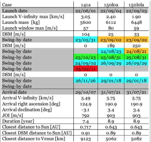
The aim of this first part of the project was to create a Python script that computes the Earth magnetic field given the coordinates and the time at which the spacefraft will reach those coordinates. In order to pursuit this purpose the data for ESA JUICE Earth fly-bys trajectories were needed. As part of the previous intership activities these trajectories have been computed and plotted through the use of Matlab and the SPICE Toolkit. For this purpose the ESA document JUICE Consolidated Report on Mission Analysis (CReMA) has been used to get the right information about the JUICE orbits. All the kernels for ESA missions can be found on the ESA SPICE website, and the files used are in the latest version available (CReMA 4.1). Different JUICE trajectory plans have been designed for the mission, but in this version of the kernels the trajectory implemented is the 141a, which assumes the launch date for 1st June 2022.
Figure 2.0.1: Main mission events table from JUICE Consolidated Report on Mission Analysis (CReMA).
In the table in figure 2.0.1 the dates of the main mission events are reported and the ones highlighted in blue are refered to the Earth Fly-bys and are taken into account in the Matlab script. The trajectories have been plotted using as reference frame GSM (Geocentric Solar Magnetospheric) in order to compare the data with some previous plots created at TU Braunschweig provided by the laboratory.
2.1
JUICE Earth fly-by trajectories
Figure 2.1.1: First JUICE Earth Fly-by designed for May 31 2023.
Figure 2.1.3: Third JUICE Earth Fly-by designed for November 26 2024.
Figure 2.1.4: All the three Earth Fly-bys plotted together around the sphere model.
In all the previous figures all the distances are in kilometers from the Earth centered reference frame. Moreover a sphere with the mean Earth radius has been added to the plots in order to have a better idea of the distances and the directions
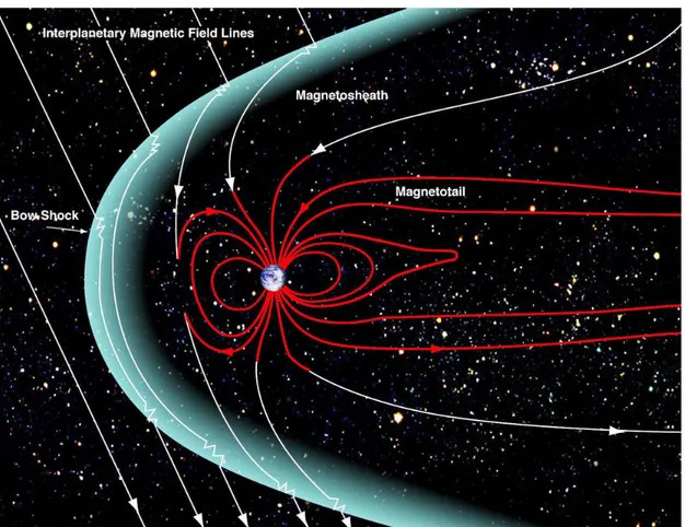
during the JUICE fly-bys. Once the trajectory coordinates have been generated, the next step has been to write a Python script that allowed to compute the Earth magnetic field data through some modules that implement the IGRF model (In-ternational Geomagnetic Refrerence field). In order to have results that could be considered reliable, different IGRF implementation modules have been taken into account. In the end the Geopack Python module has been used since it allows to implement in addition to the IGRF magnetic field also the contribution of the Tsyganenko models. The version of IGRF used is the 13th edition released in 2019 that is valid from 1900 to 2025. These models are semi-empirical best-fit repre-sentations for the magnetic field, based on a large number of satellite observations (IMP, HEOS, ISEE, POLAR, Geotail, GOES, etc). The Tsyganenko models in-clude the contributions from major external magnetospheric sources: ring current, magnetotail current system, magnetopause currents, large-scale system of field-aligned currents and solar wind.
Figure 2.1.5: A schematic view of the Earth magnetosphere deformed by external contri-butions. [NASA]
2.2
TU Braunschweig Magnetic field data
As already anticipated, the data for the ESA JUICE Earth fly-by magnetic field predictions have been also previously computed by the TU Braunschwieg and provided by the laboratory thanks to the partership for the development and the testing of JMAG. The following plots have been used in order to have a reference during the data generation process with the Python script and for comparison.
Figure 2.2.2: JUICE Earth second fly-by magnetic field prediction
The three previous figures show in a simple way the three different components of the Earth magnetic field in function of the time (and hence also the position of the JUICE) during the fly-bys. It is also shown the profile corresponding to the topocentric distance of the spacecraft in order to have an idea of the correlation between distance and magnetic field. As shown in figure 2.2.1 for the first fly-by (30 - 31 May 2023) it’s possible to see that the maximum value of |B| is 1669.6 nT and the minimum distance reached is 2.995 Earth radii, which correspond to 12719.20 km of altitude. In figure 2.2.2 for the second fly-by (1 September 2024) it’s possible to see that the maximum value of |B| is 12478 nT and the minimum distance reached is 1.305 Earth radii, which correspond to 1942.88 km of altitude. In figure 2.2.3 it is reported that the IGRF13 and TS04s models that have been used were non valid to compute data for the year 2026, so the year 2025 has been used. For the third fly-by it’s then possible to see that the maximum value of |B| is 7012.5 nT and the minimum distance reached is 1.579 Earth radii, which correspond to 3682.45 km of altitude.
2.3
Python script Magnetic field data
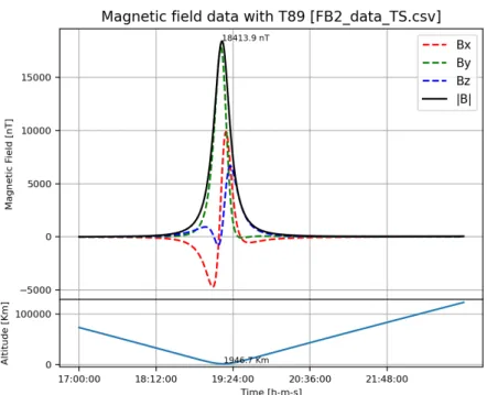
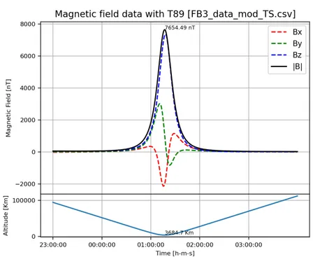
In the three following figures the Earth magnetic field data computed through the use of the Python script are shown. The script uses Geopack module, as already anticipated, in order to compute the Earth magnetic field taking also into account the T89 Tsyganienko model. The plots have been generated in a similar way to the ones from TU Braunschweig in order to have an easier comparison between the previous profiles and the values reached with the Python script. It is also shown the profile corresponding to the altitude of the spacecraft in function of the timeseries of the Earth fly-by in exam. For the case of Python script data, since the Earth radius is not constant due to its real shape, it has been necessary to get the a precise value of the altitude of the spacecraft with the function ”cspice_recpgr” from SPICE Toolkit, which transforms coordinates from cartesian to Latitude-Longitude-Altitude format.
Figure 2.3.1: JUICE Earth first fly-by magnetic field computed with the Python script.
Figure 2.3.3: JUICE Earth third fly-by magnetic field computed with the Python script.
As shown in figure 2.3.1 for the first fly-by (30 - 31 May 2023) it’s possible to see that the maximum value of |B| is 1706, 16 nT and the minimum altitude reached is 12719.9 km. In figure 2.2.2 for the second fly-by (1 September 2024) it’s possible to see that the maximum value of |B| is 18413, 9 nT and the min-imum altitude reached is 1946.7 km. For the plot in figure 2.3.3, since also the Geopack package was not valid to compute data for the year 2026, the year 2025 has been used. The procedure is the same used for plot of the third fly-by from the TU Braunschweig and the purpose of this was not to have precise prevision of the Earth magnetic field data, but instead to have just an idea of the possible reachable values. For the third fly-by it’s then possible to see that the maximum value of |B| is 7654, 49 nT and the minimum altitude reached is 3684,7 km.
2.4
Data comparison
In the following the numbers from the previous data computations have been reported and compared to have a better idea about the similarities of the two models used. In order to have a better comparison between the TU Braunschweig data and the Python script data the topocentric distances have been converted to altitudes in kilometers.
Figure 2.4.1: Summary of magnetic field data from TU Braunschweig.
Figure 2.4.2: Summary of magnetic field data from Python script.
Figure 2.4.3: Summary of absolute and relative errors between.
As it shown the values of the distances computed are almost identical, so with very small relative error. Also the computation of the magnetic field for the three Earth fly-bys are similar expecially in the first and in the third fly-by. For the second fly-by there is a bigger difference for the values of the magnetic field, which lead to a relavive error of 47.56%. This problem may be correlated with the fact that the Tsyganenko models are used in the two cases are slighlty different or maybe, since comparing the data from Python and from TU Braunschweig it is
possible to see that the values of the magnetic field components are very similar, the data from TU Braunschweig may be incorrect. For this reason, in order to have another source to use for the comparison of the Earth fly-by magnetic field data, it has been possible to have the access to the presentation of a project of two students of the Imperial College of London. These students worked on the use of the Python Geopack to compute the same trajectory for the JUICE Earth fly-bys.
Figure 2.4.4: Summary of JUICE Earth fly-by magnetic field data from the two Imperial college students Rebecca Dunkley and Verity Cook.
In this case, only the profiles in figure 2.4.4 have been provided, but looking at the plots its possible to see that the results obtained by these students are almost coincident with the ones obtained through the use of the Python script developed. It can be then reasonable to assume that the data for the second Earth fly-by computed by TU Brauschweig may be uncorrect.
Since the Python script can be assumed precise it is now possible to cosider it a starting point for the further investigation of the calibration process and the reduction of the magnitude of in-flight errors.
Chapter 3
Cluster data comparison and
development of a calibration script
In the previous chapter the Python script that computes the Earth magnetic field components for a given trajectory in a period of time has been introduced. It has been already compared to some prediction data so, for the next step of the project it has been necessary retrieve the magnetic field information from the ESA Cluster II mission in order to have a comparison with real data and to develop a calibration script in Matlab. This activity has been planned also in order to have an additional proof of the potential and the reliability of the Python script.
3.1
ESA Cluster II mission
Cluster II is an ESA space mission is currently investigating the Earth’s mag-netic environment and its interaction with the solar wind. In order to fulfill this purpose, Cluster is constituted of four spacecraft that fly in a tetrahedral con-figuration. The separation distances between the spacecraft it’s between 600 km and 20000 km. The science data from Cluster are useful in order to expand our knowledge of space weather, space plasma physics and the Sun-Earth connection. This mission has also been very useful in improving the modeling of the Earth magnetosphere.
Figure 3.1.1: ESA Cluster II space mission logo.
Each satellite carries a scientific payload of 11 instruments to study the small-scale plasma phenomena in the most relevant regions: solar wind, bow shock, magnetopause, polar cusps, magnetotail, plasmapause boundary layer and over the polar caps and the auroral zones.
• The bow shock is the region in space between the Earth and the sun where the solar wind slow-down before being deflected around the Earth. In passing through this region, the spacecraft make measurements for the characteriza-tion of the aspects than happen at the bow shock.
• Behind the bow shock is the thin plasma layer separating the Earth and solar wind magnetic fields called magnetopause that moves continuously due to the constant variation in solar wind pressure. The magnetosphere should be an impenetrable boundary. However, plasma has been observed crossing the magnetopause from the solar wind. Cluster’s four-point measurements make it possible keep tracking the motion of the magnetopause in order to study the mechanism for plasma penetration from the solar wind.
• Near the poles of teh two Earth hemispherea, the magnetic field of the Earth is perpendicular to the magnetopause, so some solar wind particles can pass through. These particles consist in ions and electrons. Cluster records the particle distributions, to characterize the phenomenon in these regions.
• The region of the Earth’s magnetic field that are stretched by the solar wind away from the Sun is the magnetotail. Cluster monitors particles from the ionosphere and the solar wind as they pass through the magnetotail area. • The precipitation of charged particles in the atmosphere creates a ring of
light emission around the magnetic pole known as the auroral zone. Clus-ter measures the time variations of transient particle flows and electric and magnetic fields in the region for the study of the well-known phonomenon of the Aurora Borealis.
In 2003 and 2004, the China National Space Administration launched the Dou-ble Star satellites, that worked jointly with Cluster to make coordinated measure-ments within the magnetosphere.
3.2
Magnetic field data comparison
For this phase of the project it has been necessary to retrieve the Earth mag-netic field data from the Cluster server. The data have been provided from the laboratory staff, which have worked on the actual mission. The idea was to find a date in which the magnetic field data could have been distincly displayed for a better visualization, so the selected time period has been between the 28th June 2014 and the 29th June 2014.
Figure 3.2.1: Magnetic field data from all the four spacecraft of Cluster for different dates including the selected time period.
In order to compare the Cluster data with the data computed through the use of the Python script first, it has been necessary to covert the Cluster data in a format that allowed to use the Geopack functions. Since the reference frame used for the coordinates of the Cluster spacecraft was the GSE, it has been necessary to convert those coordinates in GSM.
Once that the coordinates have been converted, giving them as input with the corresponding time series, the Earth magnetic field have been computed and then plotted together by components in figure 3.2.3.
Figure 3.2.2: Trajectories of the four Cluster spacecraft during the Earth fly-by of the 28th-29th June 2014.
Figure 3.2.4: Comparison between the modulus of the Cluster data and the Python script data.
Figure 3.2.5: A closer look to the modulus of magnetic field components for the first spacecraft SALSA Earth fly-by for shorter time period for both Cluster and Python script.
As it shown in figure 3.2.3 and figure 3.2.5 the results difference between the Cluster data and the ones from the IGRF model of the Geopack are quite similar for all the components. In figure 3.2.5 it has been reported the same plot of the magnetic field components but with a shorter period of time in order to have a better look at the time interval corresponding to the clostest part of the Cluster Earth fly-by. The fact that the profiles are so similar gives another proof of the efficiency of the Python script in computing Earth magnetic field data.
3.3
Calibration script
Once got a first comparison between the Cluster data and the Python script data, it has been necessary develop a Matlab script that computes the calibration matrix in order to correct the magnetic field data from Cluster to make them co-incide with the data from the Python script.
It is reasonable to assume that the only contributions to the discrepancy between IGRF data from Python script and the Cluster data are the misallignment error and the scaling error, since the offset contribution is fairly low compared to the others. This is due to the fact that usually the major contibutors for the offset errors are the Soft and Hard Iron effect. It will be shown that the Soft Iron effect has a very low impact on the overall magnetic moment vector, and the Hard Iron effect instead can easlily been taken into account in the calibration process on ground, making possible to have in general a very low offset error.
Calling F the 3xn matrix containing the XYZ components of the magnetic field from the Python script at each time step, calling W the 3xn matrix containing the XYZ components of the magnetic field from Cluster and calling C the unknown calibration matrix, in the following relationship it is shown the connection between all these matrices:
F = C · W
In the matlab script a solution in the sense of the least-squares has been com-puted to reach the closest approximation possible.
Figure 3.3.1: Calibrated magnetic field components for the first spacecraft SALSA Earth fly-by for the selected time period compared with the Python script data.
Figure 3.3.2: Residuals computed between the calibrated Cluster data and the Python script data.
As it shown in figure 3.3.1 it’s possible to see that the approximation obtained through the use of the computed calibration matrix it’s very precise. More specif-ically in figure 3.3.2 it’s possible to see that the residuals computed between the Cluster data and the solution with the calibration matrix are in a range between 30 nT on a scale with a maximum absolute value that reaches -858.35 nT . This means that the relative error is arround 0.97%.
With this calibration script is now possible correct the Cluster magnetic field data in order to reach values that are the closest possible to the ones expected. This can give a direct confirmation of the overall alignment or even reduces the alignment error, which can change after the launch or if the boom deployment does not meet its pointing requirement.
3.4
A particular solution for the Cluster
trajecto-ries
The original idea was to generate the Cluster data for the period between 28th June 2014 and 29th June 2014 using GSM (Geocentric Solar Magnetospheric) as reference frame for the coordinates of the spacecraft in order to have an easier and more direct comparison between the Earth magnetic field data from Cluster and the ones generated by the Python script. During the process of plotting the trajectories of the spacecraft a strange phenomena has been noticed.
Figure 3.4.1: The anomalous trajectories for the Cluster spacecraft from the data gener-ated with respect to the GSM frame of reference.
In figure 3.4.1 it is shown that the trajectories generated have a very unusual shape. These orbit data brought consequently to the data profiles shown in fig-ure 3.4.2.
Figure 3.4.2: Components of the position of the first Cluster spacecraft for the data generated in GSM.
The FORTRAN code that generates the spacecraft positions is actually pro-vided to all the teams working in the laboratory by ESA. The positions of the spacecraft should have been easily retrievable and no errors of this kind were ex-pected. For this reason further investigation will be done in the near future in
order to identify and correct the possible bug inside the FORTRAN code. In or-der to overcome this issue the Earth magnetic field data from Cluster have been generated, as already anticipated, in GSE.
Chapter 4
Experimental test for the
reproduction of the Earth Magnetic
field components for the ESA
JUICE Earth fly-bys
For this project, everything started with retreiving the trajectories for the ESA JUICE Earth fly-bys and the magnetic field components forecast for those fly-bys. In this chapter the last part of this scientific project will be shown. In fact the aim of this last step has been to replicate with the Space Magnetometer laboratory’s instrumentation the magnetic field components associated to each fly-by. One of the reasons of this experiment has been to test a Python script developed in order to control the scientific instrumentation to achieve the values for the magnetic field expected during the in-flight calibration process.
4.1
Instrumenation used
In order to perform this experiment what is basically needed is a coil with a known length and number of turns (that define the coil constant). The user can control the current that passes through the coil and he can then control the generation of magnetic field. The coil used has a constant of 2200 nT/mA, which means that for 1 mA of current that passes through the coil 2200 nT of magnetic field will be generated. This cylindrical coil is contained in a can made of Mu-metal, a metal alloy with a very high magnetic permeability that is very effective at blocking external magnetic fields. The can containing the coil is then contained in a wooden box as it can be seen from the figure 4.1.3.
Figure 4.1.1: The HACM Sensor used for the experiments
Figure 4.1.2: The HACM sensor fitted inside the MU-metal can. The coil is attached to the internal part of the can.
Figure 4.1.3: Wooden box containing the can in Mu-metal with the cylindrical coil inside.
Figure 4.1.4: Most relevant parameters from Keithley 6221 data sheet.
The instrument used to create and control with a very high degree of precision is the Keithley 6221 (figure 4.1.5), which is capable to work in ranges that go from 2 nA to 100 mA of AC/DC current (see figure 4.1.4). The instrument is controlled from the execution of a Python script that has been specifically modified for this
experiment, and it is then connected to the computer via a GPIB to USB converter (figure 4.1.6), which allows the user to expose the GPIB bridge to the COM port directly and control the current source. The magnetic field is then measure by a high precision fluxgate magnetometer that has been calibrated to a high accuracy called HACM (High Accuracy Calibration Magnetometer, with 0.05 nT of abso-lute accuracy). It also important to report that the HACM is very sensitive to the magnetic noise and disturbances coming from external sources.
Figure 4.1.6: The GPIB to USB converter used for the experiment.
4.2
Experiment results
The planned experiments consist in the reproduction of the X,Y and Z compo-nent of the magnetic field for all the three JUICE Earth fly-bys through the use of the cylindric coil. The data are then to be compared with the profile of the magnetic field components created through the use of the Python script with the Geopack. In order to have a deeper analysis of these fly-bys, for each of them three experimental measurements have been performed, one per each axis. Since the ac-tual duration of the fly-bys can be quite long (from 4 to 8 hours for JUCE Earth fly-bys) it has been necessary to adapt the experiment duration in order to be able to perform all the nine experiments. In fact each experiment was supposed to last about 5 minutes with a series of 150 points, having then a separation between each point of 2 seconds. To each point is associated a value of the current that the Keithley had to receive as input in order to generate the expected magnetic field.
Figure 4.2.1: Comparison between the profiles of the computed magnetic field and the experimental data for the first fly-by.
Figure 4.2.2: Comparison between the profiles of the computed magnetic field and the experimental data for the second fly-by.
Figure 4.2.3: Comparison between the profiles of the computed magnetic field and the experimental data for the third fly-by.
Figure 4.2.4: Table with the comparison between the maximum and the minimum values of magnetic field for each component of the first fly-by.
Figure 4.2.5: Table with the comparison between the maximum and the minimum values of magnetic field for each component of the second fly-by.
Figure 4.2.6: Table with the comparison between the maximum and the minimum values of magnetic field for each component of the third fly-by.
Figure 4.2.7: Relative errors for the peaks of maximum and minimum magnetic field for the first fly-by
Figure 4.2.8: Relative errors for the peaks of maximum and minimum magnetic field for the second fly-by
Figure 4.2.9: Relative errors for the peaks of maximum and minimum magnetic field for the third fly-by
In the figure figure 4.2.4, figure 4.2.5 and figure 4.2.6 it is possible to see that the profiles of the measured data are discretized. This is due to the fact that for each time step it is assigned a single value of current, thus magnetic field through the use of the coil. The spikes on the profiles are due to the fact that the HACM sensor is very sensible to the magnetic perturbation that can be present in the laboratory, as already anticipated. In the figure figure 4.2.7, figure 4.2.8 and fig-ure 4.2.9 the relative errors for the peaks of maximum and minimum magnetic field for all the components of each fly-by.
The expected relative error was about 1% but as it can be seen the relative errors are lower than 0.2%. The only exeption is the case with 3.6% of relative error
(minimum value of the Z component of the third fly-by) but, since the two com-pared values are close to 0 nT the measurement has been more sesitive to magnetic noise and calibration errors.
These experiments, which conclude the analysis of the Earth magnetic field for the ESA JUICE Earth fly-bys, can be then considered succesful as they also prooved the high level of precision of the instrumentation in the laboratory, escpecially for the Keithely 6221 and the for the HACM. This last one in fact, is the instrument that is resposable for the on ground calibration before the delivery of JMAG, giv-ing it then the same accuracy of 0.05 nT .
In conclusion it can be said that the accurate reproduction of these data confirms the ability of control of the script developed for these experiments. In fact the script will let to operate the magnetometer along an Earth fly by trajectory and calibrate the gain factor for the actual expected profile, reducing then the gain error and increasing the precision of the measurements.
Chapter 5
JACS coils Ansys simulations
As a deepening into the reasons of a calibration process for JMAG, it has been decided to investigate the influence of the Soft Iron effect on the functioning of the JMAG Calibration Alignment System (JACS) with respect to the influence of Hard Iron of the instruments on the spacecraft. In fact these effects are important in the determination of the disturbances that affects then the calibration process. These two coils that compose JACS (MX and MY) are designed to emit a mag-netic field of known size and orientation relative to the spacecraft. The field will then be measured and from this information it will be possible to calculate the orientation of the sensor reference frame directly with respect to the spacecraft frame, and thus add this orientation correction to the overall calibration matrix. This aspect is very important because it is mandatory to know the orientation relative to the spacecraft to a very high precision in order to get reliable science data. The program used to perform these simulations is Ansys through the use of the Magnetostatic module. This program has been chosen because it is easy to use for the cases of geometry design and FEM analysis management. In fact the coils geometry are quite particular so it has been chosen to use a simulation program rather than a simple analytical formula.
5.1
Soft Iron and Hard Iron effect
Soft iron is a term refering to those irons that have low carbon content and are easily magnetized and demagnetized. It is used to make the cores of solenoids and other electrical equipments. When a bar of non-magnetized iron is placed into a magnetic field, the magnetic domains shifted towards the direction of a magnetic field can be shifted back to the initial state. In soft iron, shifting of domains is
reversible, but the returned magnetic domain will align in a random manner. It can be said then that the magnetic domains of soft iron do return to the starting point when magnetic field is removed. Hard iron is instead a term refering to those irons which are not readily magnetized by induction but which retains a high percentage of the magnetism acquired. When a bar of non-magnetized iron is placed in magnetic field, the direction of magnetization of the magnetic domains tends to move towards the direction of the field. This makes the domains aligned with the direction of the magnetic field. In hard iron, the shifting of these magnetic domains is irreversible. It can be assumed then that the magnetic domains of hard iron do not return to the starting point when magnetic field is removed.
5.2
Layout of the model
Figure 5.2.1: Layout of the X and Y coil of JACS with the relative positions of MAGOBS and MAGIBS sensors.
In figure 5.2.1 the layout of the JACS coils is shown together with the positions of the sensors MAGOBS and MAGIBS with the reference frame used.
Figure 5.2.2: Coordinates for the corners of The JACS X coil refered to the S/C reference frame.
Figure 5.2.3: Coordinates for the corners of The JACS Y coil refered to the S/C reference frame.
Figure 5.2.4: Coordinates for the position of MAGIBS refered to the S/C reference frame.
Figure 5.2.5: Coordinates for the position of MAGOBS refered to the S/C reference frame.
In figure 5.2.2, figure 5.2.3, figure 5.2.4 and figure 5.2.5 are reported the coordi-nate used to design the model for the simulations. For both the cases the coils are made of copper alloy and they have been designed in order to simulate 15 turns with a section area of 136.85 mm2. The current values used istead are of 2.064 A
for the X coil and of 2.318 A for the Y coil.
Figure 5.2.6: Model layout used for the Ansys simulation with the X coil MX and the positions of MAGIBS and MAGOBS with respect to the S/C frame of reference.
Figure 5.2.7: Model layout used for the Ansys simulation with the Y coil MY and the positions of MAGIBS and MAGOBS with respect to the S/C frame of reference.
In both figure 5.2.6 andfigure 5.2.7 the coorndiate system near to the coils is the S/C reference frame used to locate all the other item in the model. Then, in order towards right, it is reported the reference frame for MAGIBS fluxgate sensor (MAG InBoard fluxgate Sensor) and the MAGOBS fluxgate sensor (MAG Out-Board fluxgate Sensor). In order to simulate the assemble in Ansys Magnetostatic it has been necessary to create a volume of study with the fuction enclosure and to create the coils as a "Multi-part component". This last action was mandatory in order to give the right direction to the corrent in the coil as shown in figure 5.2.8.
Figure 5.2.8: Representation of the direction of the current for each segment that com-poses the coil.
5.3
Simulation results
Since the JACS coils are designed to work one at a time it has been chosen to perform two different simulations, one for the X coil MX and one for the Y coil MY. This aspcet has been useful for icreasing the nuber of FEM elements dedicated to each simulation.
Figure 5.3.1: Magnetic field data for the case of MX measured by MAGIBS and MAGOBS.
Figure 5.3.2: Magnetic field data for the case of MY measured by MAGIBS and MAGOBS.
As it can be seen from figure 5.3.1 and figure 5.3.2 the X coil MX is the one that has an higher effect on the MAGIBS and MAGOBS fluxgate sensors. For this rea-son, since an environment with an higher magnetic field is capable to magnetize more the ferromagnetic materials on the spacecraft, the following computations have been performed only for the worst case scenario MX.
5.4
Computation of the magnetic field for the
fer-romagnetic materials
The next step in this study is to compute the magnetic field coming from the ferromagnetic materials, which will then have an effect of the fluxgate sensors. To do this it has been necessary to use a Matlab script that models a magnetic dipole and computes the magnetic field giving as input the absolute value of magnetic moment vector m and the position of the sensor. The magnetic moments used have been taken from a table created by Airbus that reports the magnetic mo-ment vector for each ferromagnetic material on the spacecraft.
The only Soft Iron element taking into account in this analysis is JANUS (Jovis, Amorum ac Natorum Undique Scrutator) because the value of magnetic moment for all the other items are low enough compared to the one for JANUS (0.2 Am2)
that can be considered negligible. The Hard Iron materials selected for this anal-ysis are instead the ones that have the absolute value of the magnetic moment vector higher that the JANUS one. For this analysis the matlab script has been modified in order to orient the dipole model associated to each Iron element to-wards MAGOBS direction, giving as input the coordinates of the Iron element (having the MAGOBS coordinates fixed). In this way is possible to generate the maximum contribution of each element in order to have a conservative point of view.
Figure 5.4.1: Magnetic moment components and distance from MAGOBS for the major Hard Iron effect contributors.
As shown in figure 5.4.1 these Hard Iron items have high values of magnetic moment compares to the JANUS one, so it has been decided to compute the magnetic field from all these Hard Iron elements togheter with and without the JANUS effect in order to see the exact influence of this last one compared to the others.
Figure 5.4.2: Magnetic field associated to each Hard Iron element.
In figure 5.4.2 the values for the magnetic field coming from the Hard Iron elements are shown and it is possible to see that the sum of all the contributions is 1.6152 nT . Using the same script for the JANUS case isolated the magnetic field found is equal to 0.0195 nT , which is fairly low with respect to the sum of all the Hard Iron items effects. With this value the total B coming from magnetised elements is 1.6235 nT .
reach a value of magnetic field from it of 0.5 nT, which is the expected magnitude of the magnetic field that JUICE will detect from the ocean below the surface of Ganymede. To do this the magnetic moment m has been increased with a step of 200 mAm2 till the achevement of the threshold of 0.5 nT.
Figure 5.4.3: Profile of the magnetic field in function of the increasing JANUS magnetic moment.
In figure 5.4.3 its possible to see the linear behaviour of the magnetic field in fuction of the magnitude of the magnetic moment m. The target value has then been reached after 26 iterations, which corresponds to a value of JANUS magnetic moment of 5200 mAm2.
To proove that pointing the dipole associated to the Iron elements is a conser-vative approach (the maximum value of the magnetic field B is expected in the exact direction of MAGOBS), in figure 5.4.5 it has been described the profile of the magnetic moment in function of the orientation. Taking into account figure 5.4.4 the rotation is described creating a dipole at each step one degree starting from the +Y axis toward the -Y axis.
Figure 5.4.4: Representation of the dipole associated to JANUS with the frame of refer-ence used to describe the rotation.
Figure 5.4.5: Coordinates for for the position of MAGOBS refered to the S/C reference frame.
It can be seen that the value of the magnetic field B is maximum in MAGOBS direction and the profile is simmetric since the starting position and the arrival position of the rotations are simmetric with respect to MAGOBS position.
Since the Hard Irons have a more continous effect in time they can be easily taken into account for the compuntation of the offsetin the calibration process because the disturbance magnitude can be considered almost constant. The Soft Irons instead, are more variable in time so this effect may be difficult to model accurately for the calibration process. In conclusion, since in order to reach a variation of 0.5 nT of magnetic field at MAGOBS it has been necessary to increase the magnetic moment of 26 times, it can be said that the effect of the Soft Irons (in this study only JANUS has been taken into account because its effect is dominant compared to the other sources of disturbance) are almost negligible compared to the effect of the Hard Irons for this mission.
Chapter 6
Conclusions
Through the development of this work it has been show different aspects of the calibration processes for magnetometers, more specifically for the JMAG. In fact, after the realization of the Python script that computes the Earth magnetic field data for the three JUICE Earth fly-bys the development of a working calibration script for the alignment analysis gave the opportunity to have a direct confirmation of the overall alignment, making then possible to reduce the error associated to three of six angles, belonging to the 12 calibration parameters. The development of the Python script to controlthe Keithley 6221 for the series of experiments on the reproduction of the magnetic field components for the JUICE Earth fly-bys will let to have the possibility to operate the magnetometer along an Earth fly by trajectory and calibrate the gain factor for the expected magnetic field profile, reducing then the associated error, in order to prepare the instrument for the next phases of the JUICE mission. The study associated with the simulations of the JACS coils field instead allowed to understand the low influence of the JANUS magnetic moment on the overall magnetic environment with respect to the Hard Iron disturbers presence, helping then to reduce the errors associated to the angles above mentioned and to the sensors offsets.
Bibliography
[1] Lorenzo Sanita’. ESA JUICE - JMAG Activities. 2020.
[2] Emil L. Kepko, Krishan K. Khurana, Margaret G. Kivelson, Richard C. Elphic, and Christopher T. Russell. Accurate Determination of Magnetic Field Gradi-ents from Four Point Vector MeasuremGradi-ents-Part I: Use of Natural Constraints on Vector Data Obtained From a Single Spinning Spacecraft. 1996.
[3] A. Boutonnet, G. Varga, A. Rocchi, W. Martens and R. Mackenzie. JUICE Consolidated Report on Mission Analysis (CReMA). 2018.
[4] Rebecca Dunkley, Verity Cook. Magnetic field measured by JUICE during Earth flybys. 2020.
[5] Brian J. Anderson, Lawrence J. Zanetti, David H. Lohr, John R. Hayes, Mario H. Acuña, Christopher T. Russell, and T. Mulligan. In-Flight Calibration of the NEAR Magnetometer. 2001.
[6] AIRBUS JUICE_DAT A_f_IABG_200406. 2020.
[7] AIRBUS Prediction of JMAG Sensor Orientation Based on JACS Field Mea-surements. 2020.
[8] Space Magnetometer Laboratory webpage,
https://www.imperial.ac.uk/space-and-atmospheric-physics/research /areas/space-magnetometer-laboratory/
[9] The Navigation And Ancillary Information Facility [SPICE], https://naif.jpl.nasa.gov/naif/
[10] TU Braunschweig website,
https://www.tu-braunschweig.de
[11] Tsyganenko Geomagnetic Field Model and GEOPACK libraries,
https://ccmc.gsfc.nasa.gov/models/modelinfo.php?model=Tsyganenko %20Magnetic%20Field
[12] Tsyganenko Magnetic Field Model and GEOPACK s/w,
https://ccmc.gsfc.nasa.gov/modelweb/magnetos/tsygan.html [13] ESA JUICE webpage,
https://sci.esa.int/web/juice [14] Airbus JUICE webpage,
https://www.airbus.com/space/space-exploration/juice-searching-for-life-on-jupiters-icy-moons.html
[15] ESA CLUSTER webpage, https://sci.esa.int/cluster
[16] COSMOS website for ESA JUICE kernels,
https://www.cosmos.esa.int/web/spice/spice-for-juice [17] Web page of the Python Geopack,
Chapter 7
Acknowledgement
It has been a long journey that lasted in total six years of my life, an incredible journey during which I have met amazing people and shared worderful experiences. It has been hard and with a lot of sacrifices but it has been a path that, going back, I would always choose to follow. I really want to thank Professor Marco Zannoni for having followed my thesis work from Italy during the last months. Also I have to thank Professor Paolo Tortora and Virginia Angelini that made possible to work at my final thesis at Imperial College of London. I really want to thank Professor Patrick Brown, Rachel Hudson and all the JMAG team at the Space Magnetometer Laboratory for the help with my thesis and especially for having accepted me even in this hard pandemic period. A big tank also to my friends and especially to Simone Brazioli that helped me to retrieve the data from my broken computer two week before the end of the term for my thesis. A huge thank to my girfriend Elisa that supported me during the two years of Master and the period of the thesis. In the end I really have to thank my family and especially my parents that supported me for all these years of university as they always did. Without all these people today I woudn’t be here, so I hope that with these few words I’ve been able to express how much I am grateful to them.
Lorenzo Sanità 8th October 2020
È stato un lungo percorso che è durato sei anni della mia vita, un incredibile viaggio durante il quale ho conosciuto persone fantastiche e con cui ho condiviso bellissime esperienze. È stata dura e con tanti sacrifici ma è stato un percorso che, tornando indietro, avrei sempre scelto di seguire. Ringrazio il Professor Marco Zannoni per avermi seguito durante il mio lavoro di tesi dall’Italia durante gli scorsi mesi. Ringrazio anche il Professor Paolo Tortora e Virginia Angelini che hanno reso possibile lavorare alla mia tesi presso l’Imperial College di Londra. Voglio ringraziare il Professor Patrick Brown, Rachel Hudson e tutto il team che lavora al JMAG allo Space Magnetometer Laboratory per avermi aiutato con la mia tesi e per avermi accettato nonostante il difficile periodo di pandemia. Un grande grazie anche ai miei amici e specialmente a Simone Brazioli che mi ha aiutato a recuperare i dati dal mio computer non più funzionante a due settimane dalla fine del mio periodo di lavoro alla tesi. Un grandissimo grazie alla mia ragazza Elisa che mi ha supportato durante il periodo della laurea specialistica e il periodo di tesi. In fine devo ringraziare la mia famiglia e specialmente i miei genitori che mi hanno supportato per tutti questi anni di università, come hanno sempre fatto. Senza tutte queste persone oggi non sarei qui, spero quindi che con queste poche parole io sia stato in grado di esprimere quanto io sia loro riconoscente.
Lorenzo Sanità 8 ottobre 2020