Università degli Studi di Catania
Scuola Superiore di Catania
International PhD
in
Nuclear and Particle Astrophysics
XXIV cycle
Multispacecraft observations of
Coronal Mass Ejections
A
NDREA
O
RLANDO
Coordinator of PhD
Tutor
CONTENTS
Introduction IV
1. Solar Phenomena 01
1.1 The corona and the solar wind...……...…..……...……...…..……... 01 1.2 Coronal Mass Ejections (CMEs)..…...……...…..……...……...…..…….. 05 1.2.1 CME‟s classification……..……...….…...…..……...……...…..….. 10 1.2.2 Halo CMEs..……...……...…..……....….……...……...…..…….... 12 1.2.3 CME‟s models……….... 15 1.3 Influence of solar phenomena on Space Weather……...……...…..…….... 18
2. STEREO Satellite 20
2.1 STEREO Mission………...……...…..……...….……...…. 20 2.2 SECCHI Instrument…..………...……..…..……...….……...……....……. 25 2.3 COR1 and COR2………..……...…..……...….……...…..…...…... 27
3. STEREO Technique 30
3.1 Stereoscopy...….……...…..…...…………...….……...…..…...………….... 30 3.2 Epipolar Geometry……...…..…...…………...….……...…..…...…………. 32 3.3 Tie-Point Reconstruction…...…...…………...….……...…..…...…………. 34 3.4 Local Correlation Tracking (LCT)………... …...………...……... 39 3.5 Coordinate System and Display of 3D Features ………..….……...…..…… 41
4. Data Analysis 44
4.1 Selection of the halo CMEs…..………...….……….…..…...…………... 44 4.2 Analysis of the halo CMEs…...….……...…..…...……….…...….……... 46 4.2.1 CME occurred on April 3, 2010...….…...…..……...……...…..……. 46 4.2.2 CME occurred on August 7, 2010…....….……...……...…..……... 63 4.2.3 CME occurred on February 15, 2010..………... 75
5. Cosmic Rays and Space Weather 88
5.1 Cosmic Rays...….………..….... 88
5.2 Forbush Decrease………....….…...….….…….…….. 90
5.3 Auger Observatory…….……….….………..…...….…....……. 93
5.4 CMEs and Forbush Decrease…...….……..………..…... 95
5.5 CME and Space Weather………..………. 97
6. Conclusions and Future Work 103
6.1 Discussion..….………..…….. 103
6.1 Conclusions……….... 106
6.2 Future Works……….………....….…...….….…….…….…..
107
Acknowledgements 109
«Se non che la scienza è vana se non è utile, e la meteorologia è fortunatamente di quelle scienze da cui l’umanità può ricever grandi ed utili servigi. È vero che lo scienziato non può impedire la formazione delle burrasche, né variare il regime delle piogge, può però cogli avvisi prevenire molti danni delle tempeste e ciò non solo in terra, ma molto più in mare»
INTRODUCTION
The Sun-Earth environment is strongly influenced by the coupling level between the Earth magnetosphere and the interplanetary magnetic field. The latter is closely related to the solar wind, a flux of plasma continuously flowing from the Sun and propagating in the interplanetary space medium. This plasma is constituted by electrons, protons and heavier particles, and propagates with a speed of 400-800 km/s, reaching Earth in 2.4 – 4.6 days.
A sudden increase of the solar wind‟s speed is achieved by two types of phenomena: flares and Coronal Mass Ejections (CMEs).
Flares are strong explosions that involve different layers of the solar atmosphere: they are due to a sudden release of energy (1022-1025J) in areas previously characterized by variations in the configuration of the magnetic field. Flares have an evolution time variating from 10 minutes to some hours. The phenomena that occurr during a flare produce heating of the chromospheric and coronal plasma and intense electric fields that accelerate charged particles.
Coronal Mass Ejections (CMEs) are expulsions of material from the solar corona and, from an energetic point of view, they reach the same order of magnitude of the flares; they can moreover pour in the space up to many billion tons of coronal plasma. Such phenomena can occur many times a day and can accelerate the solar plasma up to 3000 km/s. Even if they have been extensively studied since their discovery, back in the „70s, a complete model for their explanation is still lacking. From our present knowledge, it seems that CMEs are strongly linked to the photospheric (sunspots, active regions), chromospheric (filaments) and coronal (flares) activity.
Starting 1996, the Large Angle and Spectrometric COronograph (LASCO) instrument, on board of the SOlar and Heliospheric Observatory (SOHO) satellite, permitted for the first time to observe the corona with a large field of view, in the range of about 1.1 to 30 solar radii. Moreover observations at different wavelengths (visible, X and EUV bands) are of primary interest in the study of a CME development from its initial phase, in lower corona, to great distances from the Sun.
The online Goddard Space Flight Center catalogue (GSFC/NASA) contains data about the CMEs observed by the LASCO coronographs when the SOHO satellite was lying in the lagrangean point L1 of its orbit. These data can nowadays be correlated to the ones taken by the two twin Solar TErrestrial RElations Observatory (STEREO) satellites, that allow a stereoscopic view of CMEs.
In this context, this thesis concerns the study of the physical processes that lie at the base of the CME formation and of their effects on the Sun-Earth environment. Such an investigation can be done utilizing data taken from satellites that study solar wind, interplanetary magnetic field, flares and CMEs.
A source of data lies in the Sun Earth Connection and Heliospheric Investigation (SECCHI) remote sensing instruments, onboard of the STEREO-A and STEREO-B satellites. SECCHI allows the realization of synchronization techniques for the two satellites and the construction of stereoscopic pictures, that can be employed to build a 3-D description of the Sun and of the 1 AU heliosphere.
Another source of data is the Michelson Doppler Imager (MDI) instrument onboard of SOHO satellite: MDI provides magnetograms that are useful to study the magnetic configuration of active regions. Moreover, the Auger Observatory and others neutron monitor stations are used for the detection of cosmic rays and for the analysis of the correlation between Forbush decreases and CMEs.
CHAPTER 1. SOLAR PHENOMENA
1.1 The Corona and the Solar Wind
The corona is the outermost region of the solar atmosphere and is located above the so-called "transition region". In the visible part of the electromagnetic spectrum, its emission is much fainter than the photosphere (about 10-6 L⊙)1 and can be commonly observed during the Sun‟s total eclipse (Figure 1), or using a special tool, called
coronagraph, which shields the solar disk simulating a total eclipse.
Figure 1. The corona during a total solar eclipse in 2008 (photo credit: Druckmüller, Aniol, Rušin). However, the solar corona appears much brighter than the photosphere outside the visible spectrum, especially in X-band, EUV and radio band. The coronal plasma is a very tenuous plasma (density of the order of 1014 particles m-3), characterized by a temperature of about 1.5-2·106 K.
The images in the X-band show that the corona consists of a set of distinct structures, which can be very different between them in terms of size and physical conditions (Figure 2).
Figure 2. The solar corona observed in X-ray from the Hinode satellite.
We can distinguish bright points (about 2∙104 km in diameter), short-lived structures (less than two days) that, unlike other typical phenomena of solar activity such as spots, are distributed evenly across the solar disk. Larger structures (≥ 105 km), of longer duration (days and weeks), which are typically associated with the spots and faculae are called bright regions, and are characterized by a higher density of particles and higher temperature than the surrounding coronal regions.
There are also other regions, commonly observed in the Sun‟s polar region and showing almost no X-ray emission, which have been called coronal holes. They have an average life of over six months and for this reason they are the most persistent solar phenomena. Coronal holes appear dark because their temperature and their density are smaller than the surrounding corona.
In the area below a coronal hole, the photospheric magnetic field is weak (~1 G) compared to surrounding regions and predominantly of the same polarity. The coronal holes are usually formed at the poles and then slowly extend to lower latitudes.
Contrary to what happens in bright regions, coronal holes rotate rigidly, so their angular velocity does not vary significantly with latitude and the rotation period decreases by only 3% from the pole to the equator, and is about 27 days.
The coronal holes are closely related to another phenomenon of the solar activity: the solar wind, a stream of plasma that flows continuously from the Sun and propagates in the interplanetary medium. In particular, coronal holes are the sources of the fast solar wind, which propagates with an average speed of 750 km/s and is relatively constant over time (Figure 3 and 4).
Figure 3. This composite image shows in the form of polar pattern the speed of the solar wind as a
function of solar latitude, measured from Ulysses spacecraft during solar minimum of the cycle 23. The speed of the solar wind is almost constant and of the order of about 750 km/s at high solar latitudes
( > 30°) while it is lower and more variable at the low latitudes. At the graph‟s speed is superimposed an image of the corona.
The slow solar wind stems from structures of closed coronal magnetic field lines, such as the streamers. They appear as large gothic arch-shaped structures that trap ionized coronal gas. The slow solar wind consists of particles moving at an average speed of 400 km/s and is highly variable (Figures 3 and 4).
Proton density 6.6 cm-3 Gas pressure 30 pPa
Electron density 7.1 cm-3 Sound speed 60 km s-1
He2+ density 0.25 cm-3 Magnetic pressure 19 pPa
Flow speed (nearly radial) 450 km s-1 Alfvén speed 40 km s-1
Proton temperature 1.2∙105 K Proton-proton time
collision 4∙10
6 s
Electron temperatue 1.4∙105 K Electron-electron time
collision 3∙10
5 s
Magnetic field (induction) 7 nT Time for wind to flow
from corona to 1 AU 3.5∙10
5 s ~ 4 days
Table 1. Observed properties of the solar wind near the orbit of the Earth (from Kivelson et al., 1995).
There are two classes of phenomena that can produce sudden increases in solar wind speed, they are the flares and the coronal mass ejections (CMEs).
1.2 Coronal Mass Ejections (CMEs)
CMEs are the most spectacular large-scale demonstration of solar activity and there is currently no single model that can fully explain this phenomenon, although several models have been proposed (Figures 5). The multi-wavelength observations are thought to be crucial to a complete understanding of CMEs [Hudson and Cliver, 2001]. Recently, it was proposed that Ly line at the ultra-violet (UV) wavelength might be very suitable for the detection of CMEs [Vial et al., 2007].
The white-light emission of the corona comes from the photospheric radiation Thomson-scattered by free electrons in the corona, and any enhanced brightness means that the coronal density somewhere along the line of sight is increased.
Figure 5. CME observed by SOHO in 2002. The image was taken by the LASCO C2 instrument, which
blocks out the Sun with an occulting disk so that we can see the fine details of the faint corona. An EIT 284 Å image of the Sun itself, taken at about the same time, is superimposed on the occulting disk.
In addition to the density enhancement, the Thomson scattered radiation depends on the photospheric radiation incident to the electrons and the angle between the incidence and the line of sight, which makes CMEs favorably observed near the plane of the sky.
With the continual observations from various ground-based and space-born coronagraphs, more than ten thousand CME events have been recorded, which enables the statistical investigation of their properties [Chen, 2011].
Since the beginning of 1996 the instrument LASCO (Large Angle Spectrometric and Coronograph) onboard the SOHO satellite, has allowed, for the first time, to observe the corona with a large field of view, from about 1.1 to about 30 solar radii (R⊙)2.
In general, the CMEs appear as eruptions of magnetic arches that connect regions of opposite magnetic polarity on either side of a photospheric magnetic neutral line3. Where it is possible to observe CMEs in the low corona, we note that most of them originated from a system of two large magnetic arches. The observations of the corona in the FeXIV emission line recently showed the almost systematic quadrupolar nature of the CME [Schwenn et al., 1997]. In fact the structure of the corona is governed by the solar magnetic field and the magnetic topology is that of a simple magnetic dipole, but often multipole components are involved.
Based on the Thomson-scattering formulae [Billings, 1966], the mass of a CME can be estimated [Hundhausen, 1993]. Without the knowledge of the exact position of the density-enhanced structure, it is often assumed that the CME is close to the plane of the sky, which would underestimate the mass of the CME.
Typically, the mass of a CME falls in the range of 1∙1011–4∙1013 kg, averaged at 3∙1012 kg [Jackson, 1985; Gopalswamy and Kundu, 1992; Hudson et al., 1996].
About 15% of the CMEs have a mass less than 1011 kg [Vourlidas et al., 2002]. The angular width of CMEs projected in the plane of the sky ranges widely from ∼ 2° to 360° [Yashiro et al., 2004], with a significant fraction in the low end (e.g., < 20°) and a small fraction in the high end (e.g., > 120°).
The observations indicate that we can divide CMEs into at least two categories. The CMEs with the angular width less than ∼ 10° can be called narrow CMEs [Wang et al., 1998], and the others are sometimes called normal CMEs [Yashiro et al., 2004] (Figures 6 and 7 show the two CME‟s categories). Note that halo CMEs (see paragraph 1.2.2), with an apparent angular width of or close to 360°, might simply due to that the CMEs, probably with an angular width of tens of degrees, propagate near the Sun-Earth line, either toward or away from the Earth.
During the solar cycle 23, the LASCO provided unprecedented observations of CMEs. The occurrence rate of CMEs was found to basically track the solar activity cycle, but with a peak delay of 6-12 months [Raychaudhuri, 2005; Robbrecht et al., 2009]. Before the SOHO era, the averaged occurrence rate was found to increase from 0.2 per day at solar minimum to 3.5 per day at solar maximum [Webb and Howard, 1994].
Figure 6. Example of a narrow CME seen in LASCO C2 data on 1999 April 24. Sun center is in the
With the increased sensitivity and wider field of view, the SOHO/LASCO coronagraph assembly, including C1, C2, and C3 components with different fields of view, detected CMEs more frequently.
Figure 7. Example of a normal CME seen in LASCO C2 on 2000 March 20 (SOHO/LASCO).
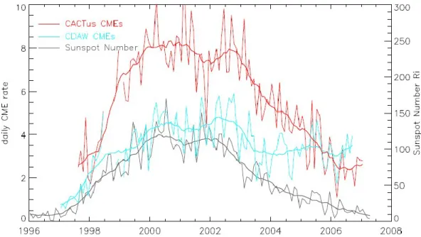
The CME catalog in the NASA CDAW data center, where CMEs are identified by eye, shows that the CME occurrence rate increases from ∼ 0.5 per day near solar minimum to ∼ 6 near solar maximum, summing up to more than 13000 CMEs during the solar cycle 23 [Gopalswamy et al., 2003; Yashiro et al., 2004].
However, for the same observational period, the automated software (CACTus) identified much more events, with the occurrence rate increasing from < 2 per day near
shows the comparison of the CME daily occurrence rate detected by the two methods, along with the sunspot number.
Figure 8. The CME daily occurrence rate detected by the CACTus archive (red) and the CDAW archive
(blue) compared with the daily sunspot number (gray) during solar cycle 23. Thin curves: smoothed per month, thick curves: smoothed over 13 months (from Robbrecht et al., 2009).
Constructing CME models is extremely important, not only because CMEs are a spectacular astronomical phenomenon, but also because they are the main driver for the space weather disturbances that strongly affect our high-tech life. It is important to emphasize here that any successful model should be based on the combination of observations and magnetohydrodynamic (MHD) theory.
The same as any other eruptive phenomenon, CMEs, along with solar flares, involve the energy conversion from one kind to the kinetic, potential, thermal, and nonthermal energies, as well as the radiative energy in flaring loops. It should be noted that there are secondary conversions between different energies, e.g., part of the nonthermal energy would be converted into the thermal energy, which would finally radiate out. They should not be double counted when estimating the CME and flare energies. With the assumption that a typical CME involves a volume of 1024 m3, the
energy density of a CME ranges from 10–2–10 J m–3. The typical energy density of possible energy sources is shown in Table 2 [Forbes, 2000].
Table 2. Estimates of the coronal energy sources.
We can see that for energetic CME events, which are the most interesting in the space weather context, the only possible source is the magnetic energy, whereas for very weak CME events, thermal and potential energies in the pre-eruption corona may contribute to the CME explosions. In the case that these two sources are available, thermal energy is converted to the CME energy by the work of pressure gradient, similar to the acceleration of solar wind, and the potential energy is converted to the CME energy in the form of buoyancy.
In those eruptive cases, the CMEs energy comes from the partial release of the magnetic free energy, i.e., the excess energy compared to the potential field with the same flux distribution at the solar photosphere. It is demonstrated that in the case of force-free field that is often applicable in the low corona [Gary, 2001], the magnetic free energy is of the order of the magnetic energy of the corresponding potential field [Aly, 1984].
1.2.1 CME’s classification
CMEs generally have a three parts structure (see Figure 9 (left)): proceeding from outside to inside, a bright loop is observed, superimposed on a coronal cavity with no emission, which in turn contains high plasma density from an eruptive prominence.
Figure 9. Two images of CMEs observed respectively by LASCO C2 (left) and LASCO C3 (right),
respectively, in which the typical CME structure in three parts and the helical structure are shown.
The observations made with the instruments onboard SOHO, EIT and LASCO C1 in particular, have shown that these three components are present in the low corona during the early stages of development of a CME. In addition, many CMEs observed with LASCO instrument showed a helical structure (Figure 9 (right)). Along with these types of CMEs, others have been identified: for example, a CME that originates at a given latitude can cause the destabilization of a multi-polar region on a larger scale, and the resulting CME can cover a range of latitude exceeding 60°.
CMEs often occur in association with flares, in which case we refer to flare-CME events. During flare-CME events, accelerated electron beams that propagate along the magnetic field lines produce radio bursts. The LASCO instrument has confirmed the existence of two classes of CMEs, which have different speeds of propagation.
The first class, called impulsive CME, is formed by the CMEs having a high speed and a small acceleration. Speeds are typically in excess of 750 km/s. Impulsive CMEs are often associated with flares and Moreton waves4 on the disk.
The second class, the gradual CME, is formed by CMEs that evolve slowly and then accelerate. Speeds are in the range of 400–600 km/s, while the accelerations measured varies from event to event and can reach up to 30 m/s2. Gradual CMEs are
4 A Moreton wave is the chromospheric signature of a large-scale solar coronal shock wave. Described as a kind of solar 'tsunami', they can be generated by solar flares.
apparently formed when prominences and their cavities rise up from below coronal streamers. The CME associated with the quiescent prominences probably fit this category. Both classes can reach speeds of 3000 km/s.
More recently, a new class of CME has been identified by LASCO. These events were seen as a slow accretion of densities that originate above the cusps of helmet streamers and move radially outward with almost constant acceleration of about 3-5 m/s2 [Sheeley et al., 1997].
They resemble small CME evolving gradually. Based on their radial motions and the slow speed increases, besides than the fact that originate in the streamer belt, Sheeley et al. [1997] have concluded that they are the traces of the flow of slow solar wind.
In order to explain the different kinematics, Low and Zhang [2002] proposed an idea for the two types of CMEs, i.e., the normal polarity flux rope eruptions correspond to the fast CMEs, whereas the inverse polarity flux rope eruptions correspond to the slow CMEs. On the other hand, it was found that, even for the inverse type only, the CME speed can be high or low [Chen and Krall, 2003; Wu et al., 2004].
1.2.2 Halo CME
As already stated, CMEs can also manifest as events that have an angular width of ~360°, and in this case they are called halo events.
These types of events were identified for the first time with the coronagraph onboard the satellite P78-1 and were defined as an increase in brightness that surrounds the solar disk [Koomen et al., 1975]. The halo events are CMEs that originate close to the centre of the solar disk and are directed along the line joining the Sun and the Earth.
It is widely accepted that they are nothing but CMEs propagating near the Sun-Earth direction, either toward or away from the Sun-Earth [Howard et al., 1982]. However, statistical investigations indicate that the average velocity of halo CMEs, ∼ 957 km/s,
is twice as large as that of normal CMEs (e.g., Yashiro et al., 2004), which seems to make halo CMEs special.
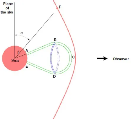
It may be natural to think that the nearly circular front of halo CMEs is just the face-on view of the dome-like CME frontal loop. For simplicity, we assume that the CME frontal loop is represented as the shell of a cone-shaped dome as illustrated by Figure 10 [Chen, 2011].
When it is observed edge-on as a limb event, it would appear as a loop structure, i.e., the green lines linking points A, B, C, D, and E, since the optical thickness is much larger here. When the CME is observed face-on as a halo event, however, the optical thickness is large only near the torus linking points B and D, i.e., the blue lines in Figure 10, which surrounds the solar disk to the observer. If so, the nature of halo CMEs would be the same as the normal CMEs.
Figure 10. A sketch showing how a dome-like CME would be observed as a limb event (green lines)
and as a halo event (blue lines). The red line ahead of the CME is a fast-mode piston-driven shock wave. is the inclination angle between the radial direction of point F and the plane of the sky, whereas is the angle between the CME leg and the plane of the sky. It is seen that the far wing, say, near point F, propagates in a direction closer to the plane of the sky than the CME does (since < ) (from Chen,
For example, Krall et al. [2006] extended the flux rope model (see Section 1.2.3), which was demonstrated to be applicable to limb CMEs [Chen, 1996; Krall et al., 2001], to halo CMEs, and found that the model can reproduce both quantitative near-Sun properties of the 2003 October 28 CME and the timing, strength, and orientation of the fields measured in situ near the Earth orbit. Of course, the nature of CME frontal loops is still under debate, and there are other possibilities, such as that the CME frontal loop is due to the compression of magnetic field lines which are stretched successively.
If the nature of halo CME fronts is the same as normal CMEs, there is a serious problem: why halo CMEs are on average twice faster than normal CMEs? Noticing that the Thomson scattering is significantly reduced for halo CMEs, Andrews [2002] proposed that many dim and slow halo CMEs are missed by coronagraphs so that the average velocity of the observed halo CMEs is high.
Following this line of thought, Zhang et al. [2010] performed Monte Carlo simulations to investigate how the white-light brightness of CMEs with an average velocity of 523 km/s is reduced when they are observed as halo events. They found that the brightness of many narrow and slow CMEs, when they are observed as full halo CMEs, is reduced to a level comparable to the solar wind fluctuations, and therefore, these events would be missed to be identified in the coronagraph images. The remaining observable halo CMEs have an average velocity of ∼ 922 km/s, quite similar to the value in observations.
An alternative view is that the halo CME fronts are completely different from the frontal loops of limb CMEs in physics. For example, Lara et al. [2006] proposed that the halo CME fronts might be the combination of the CME-driven shock wave and the CME material itself. Based on MHD numerical simulations, Manchester et al. [2008] synthesized the white-light images of a halo CME event, and found that the halo CME front can be identified as the CME-driven shock wave.
Since the fast-mode wave in the corona is of the order of 1000 km/s, it easily explains why the average velocity of halo CMEs is as high as 957 km/s. One may argue that the piston-driven shock wave is much weaker in white light than the CME
frontal loop, and therefore can be barely visible in the coronal images. This is true for the limb events (e.g., Vourlidas et al., 2003).
However, for halo CMEs, as illustrated by Figure 10, the situation may change. If we consider the Thomson scattering, which remarkably favors the plasma moving in a direction closer to the plane of the sky, the scattered white-light emission of the shock wave front at point F in Figure 10 could be stronger than that of the CME frontal loop near point B when both points are observed at the same projected heliocentric distance in the plane of the sky, although the plasma density is higher at point B than point F.
1.2.3 CME’s Models
The study of the CMEs has not yet allowed us to establish with certainty what is the mechanism responsible for the formation of such events. The knowledge gained through observations have led to discard the possibility of a mechanism due to a sudden increase of the plasma pressure. Current models consider a mechanism driven by a magnetic force.
Low [1996] developed a model in which a CME is a magnetic flux rope5 expulsion which is gravitationally confined within the cavity of a helmet streamer. At a certain moment this twisted magnetic flux tube becomes unstable and starts to rise towards the outer layers of the atmosphere and blows off breaking helmet streamer‟s field lines. This study led to the elaboration of a three-dimensional MHD flow of a flux rope, and simulations show the characteristic three components structure of the CME (Figure 11).
5 A magnetic flux rope can be defined as a structure consisting of magnetized plasma, with a shape similar to a twisted rope (see Figure 11).
Figure 11. The evolution of the magnetic field in the 3D MHD numerical simulation of Amari et al.
[2000], which shows the formation and eruption of a twisted flux rope as a simple magnetic arcade experiences shearing motions and the opposite-polarity magnetic emergence.
Another line of research considers the presence of a global instability (catastrophe
model). A possible magnetic configuration is characterized by a twisted magnetic flux
tube enclosed in an arch (Figure 12).
The photospheric motions or the weakening of the magnetic field can bring the system to a point of non-equilibrium and the flux tube rises rapidly. It then forms a current sheet in the region below and this induces a process of magnetic reconnection so that the flux tube is ejected. This evolution can take place in a bipolar magnetic configuration, but it is more likely to occur in a quadrupolar configuration.
Figure 12. Catastrophe Model. Evolution of a twisted flux tube. Figure on the right, from bottom to top:
the flux tube is initially in equilibrium near the photosphere; the evolution of the photospheric flow takes the system to a critical point with the formation of a current sheet below. Magnetic reconnection takes place changing the topology of the field (left), and the twisted flux tube is then expelled (adapted
from Forbes and Priest, [1995]).
A different approach was adopted by Antiochos et al. [1999], that assume a topology of quadrupolar field (break-out model) (Figure 13).
When the lower central arch is sheared, it extends up through contact with the arch above it, forming a current sheet. It is assumed that the reconnection takes place initially with a low efficiency, the distorted arch is bounded by the highest and that the magnetic energy is progressively stored.
Figure 13. Break-out model. In the first figure on the left there is the potential quadrupolar
configuration (the field is symmetrical about the axis of rotation and the equator). In the two following figures the system evolves due to photospheric distortion that is applied to the lower part of the central
When the efficiency of reconnection becomes significant, the confinement of the upper arcade fails, while the lower arcade spreads rapidly upwards.
The complexity of the observed CMEs requires the development of more realistic models. A plausible configuration consists of a twisted flux tube enclosed in a large quadrupolar region. This model is the combination of a catastrophe model [Forbes and Priest, 1994, Lin et al, 1998] with a break-out model [Antiochos et al, 1999], where the kinked arch is replaced by a twisted flux tube.
However, none of these models explains the wide variety of CMEs observed.
1.3 Influence of solar phenomena on Space Weather
The solar wind and the magnetic field frozen in it, produce many effects on Earth, such as, for example, variations of the geomagnetic field (geomagnetic storms), of the currents flowing in the magnetosphere-ionosphere system (geomagnetic substorms, auroras) and of the flow of high energy charged particles (in the polar regions). These effects are now framed within a context that is called Space Weather. The term Space Weather has been coined to emphasize how the solar activity and the conditions of interplanetary space can have a direct impact on the terrestrial environment and also on daily life, so it is important to study and possibly forecast these conditions. The solar wind is responsible for the so-called auroral oval, a thin halo of permanent light of 4000 km in diameter that surrounds the Earth's magnetic poles at a height of about 110 km.
The most evident effect of geomagnetic activity is the increase of the ionospheric current system along the auroral oval which moves toward the equator. As a result, significant increases in current (sometimes even millions of Amperes) can be induced in long conductors of artificial nature, such as power, gas and oil pipelines. In the case of oil and gas pipelines, local damage may occur due to electro-corrosion. In the case of the power lines, other than the damages caused by the dissipation of energy delivered, if the induced current reaches transformers, they can also destroy them, causing major blackouts. Malfunctions due to induced currents induced by
disturbances of the ionosphere have been repeatedly found in railway signaling systems, particularly in Finland and Canada.
It should also be reminded the influence on "normal" mobile phone, without the use of satellites. Providers tend to deny firmly, but there are studies at the New Jersey Institute of Technology/Bell Labs, showing that during the strong solar activity, when there is an alignment between the Sun, distribution cell phone and mobile device (especially when the sun is low on the horizon), can occur that the solar radio emissions deceive the cell, losing the attachment to the cell in use. This phenomenon is not really dramatic for our daily activities. However it exists and probably will be more important with the development of mobile networks of third generation (UMTS). The other serious consequence of disturbances in space weather is the chance of a damage to satellites in orbit around the Earth. In fact, it may cause faults to internal electronic components or damage of the surface of the satellite (especially critical are the photovoltaic panels that provide power). For example, broadcasting satellites, which provide connections to the telephone and television programs, depend on space weather. Other things that are harmful to the satellites are repeated passages through the Van Allen6 radiation belts (the intensity of the radiation belt is related to space weather) and the debris left by comets and humans. High-energy particles can also endanger the health of the astronauts onboard, for example, the Space Shuttle or space station in orbit, and in case of intense events may also affect passengers on airliners flying over the polar routes.
6 The Van Allen radiation belts are regions of high density of charged particles surrounding Earth. The belts are made of very energetic electrons and protons. The inner belt is made up of high-energy protons (10-100 MeV), while the outer belt is formed by protons and electrons of lower energy (1-10 MeV).
CHAPTER 2. STEREO SATELLITE
2.1 STEREO Mission
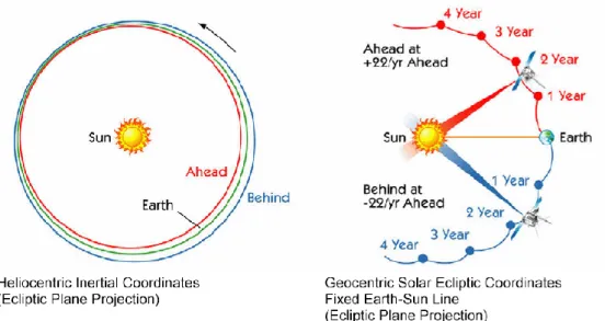
The twin NASA STEREO (Solar Terrestrial RElations Observatory) spacecraft (A and B) were launched on a single Delta rocket from Cape Canaveral on October 25, 2006. Using a lunar encounter, each spacecraft was inserted into an individual final orbit, one spacecraft (B) gradually falling behind Earth in orbit and the other (A) increasingly ahead of Earth. The two spacecrafts drift away from Earth at an average rate of about 22.5 degrees per year (Figure 14). After the two year nominal operations phase the spacecraft were about 90 degrees apart, each about 45 degrees from Earth. STEREO-A had to drift ahead of Earth and STEREO-B behind. In order to accomplish this drift, STEREO-A had to be travelling faster than Earth around the Sun and so must have had an orbit slightly closer to the Sun than Earth's. Similarly, the STEREO-B had to be travelling slower than Earth and must have had an orbit slightly further than Earth.
Figure 14. A sketch showing the positions of the two STEREO satellites taken during the first years.
known as quadrature. This is of interest because the mass ejections seen from the side on the limb by one spacecraft can potentially be observed by the in situ particle experiments of the other spacecraft.
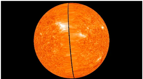
As they passed through Earth's Lagrangian points L4 and L5, in late 2009, they searched for Lagrangian (trojan) asteroids (Figure 15). On February 6, 2011, the two spacecraft were exactly 180 degrees apart from each other, allowing the entire Sun to be seen at once for the first time (Figure 16).
Figure 15. Image shows the position of STEREO satellites near Earth's Lagrangian points L4 and L5 in
August 2009.
The STEREO mission is the third in the line of Solar-Terrestrial Probes (STP) and is a strategic element of the Sun-Earth Connections Roadmap. STEREO is designed to view the three-dimensional (3D) and temporally varying heliosphere by means of an unprecedented combination of imaging and in situ experiments mounted on virtually identical spacecraft flanking the Earth in its orbit.
The primary goal of the STEREO mission is to advance the understanding of the three-dimensional structure of the Sun's corona, especially regarding the origin of coronal mass ejections (CMEs), their evolution in the interplanetary medium, and the dynamic coupling between CMEs and the Earth environment.
Figure 16. Image of the far side of the Sun based on high resolution STEREO data (EUVI 304 Å), taken
on February 2, 2011 at 23:56 UT when there was still a small gap between the STEREO Ahead and Behind data. This gap started to close on February 6, 2011, when the spacecraft achieved 180 degree
separation, and completely closed over the next several days (NASA).
We recall that CMEs are the most energetic eruptions on the Sun, are the primary cause of major geomagnetic storms, and are believed to be responsible for the largest solar energetic particle events.
The STEREO suite has three main parts (Figure17): the SCIP (Sun Centered Imaging Package - three telescopes), the HI (Heliospheric Imager - two telescopes) and the SEB (Secchi Electronics box) [Howard et al., 2008].
Each of the spacecraft carries cameras, particle experiments and radio detectors in four instrument packages:
Sun Earth Connection Coronal and Heliospheric Investigation (SECCHI) has five cameras (Figure 18): an extreme ultraviolet imager (EUVI) and two white-light coronagraphs (COR1 and COR2). These three telescopes are collectively known as the Sun Centered Instrument Package or SCIP, and image the solar disk and the inner and outer corona. Two additional telescopes, heliospheric imagers (called the HI1 and HI2) image the space between Sun and Earth. The purpose of SECCHI is to study the 3-D evolution of Coronal Mass Ejections through their full journey from the Sun's surface through the corona and interplanetary medium to their impact at Earth (Figure 19).
In-situ Measurements of Particles and CME Transients (IMPACT) can study energetic particles, the three-dimensional distribution of solar wind electrons and interplanetary magnetic field.
PLAsma and SupraThermal Ion Composition (PLASTIC) can study the plasma characteristics of protons, alpha particles and heavy ions.
STEREO/WAVES (SWAVES) is a radio burst tracker that can study radio disturbances traveling from the Sun to the orbit of Earth.
Figure 18. A close-up of the spacecraft body showing the EUVI, COR1-2 and HI telescopes, together
with the SECCHI Sun Centered Instrument Package (SCIP). (Adapted from diagrams by the Johns Hopkins University Applied Physics Laboratory).
Figure 19. Composite of STEREO-A and B images from the SECCHI instruments of the CME of 12
December 2008. Image shows that the CME is Earth-directed, being observed off the east limb in STEREO-A and off the west limb in STEREO-B (adapted from Byrne et al., 2010).
2.2 SECCHI Instrument
SECCHI is named after one of the italian astronomer: Angelo Pietro Secchi (1818-1878), a Jesuit priest. He was one of the first astrophysicists to use the new medium of photography to record solar eclipses. He photographed the 1860 eclipse, during which a CME is now thought to have occurred (see Figure 20).
Figure 20. Eclipse drawings showing a possible CME (Angelo Secchi, 1860).
SECCHI is a suite of 5 scientific telescopes that observe the solar corona and inner heliosphere from the surface of the Sun to the orbit of Earth.
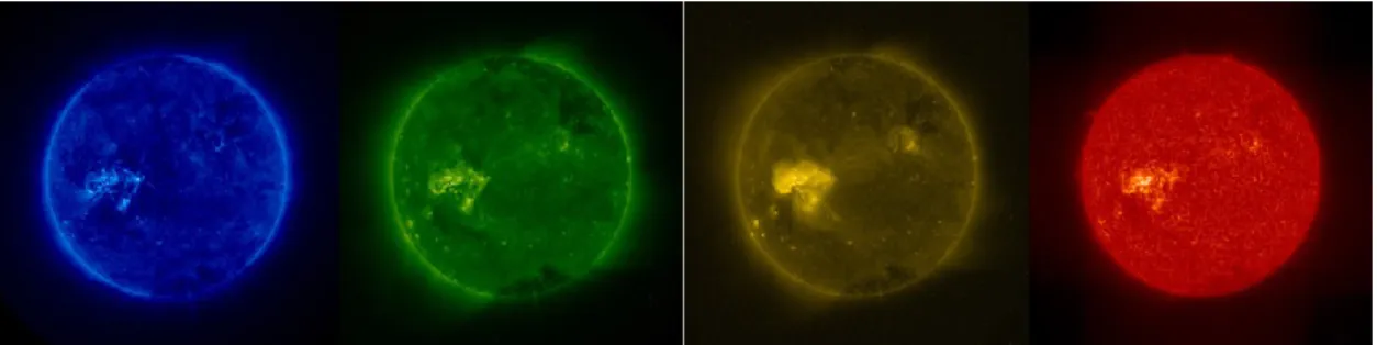
The EUVI telescope was developed at LMSAL (Lockheed Martin Solar and Astrophysics Laboratory). The EUVI observes the chromosphere and low corona in four different EUV emission lines between 17.1 and 30.4 nm. It is a small, normal-incidence telescope (Ritchey-Chrétien system) with thin metal filters, multilayer coated mirrors, and a back-thinned CCD detector. The Extreme Ultra-Violet Imager obtains full disk solar images in four EUV wavelengths (17.1, 19.5, 28.4, 30.4 nm)
(Figure 21), producing images with a cadence as fast as 2.5 minutes in the most common wavelengths.
Figure 21. Views of the Sun from STEREO/EUVI in the four wavelengths (17.1, 19.5, 28.4, 30.4 nm,
respectively from left to right) (NASA/STEREO).
Heliospheric Imagers (HIs) consists of two small, wide-angle telescope systems mounted on the side of each STEREO spacecraft, which view space, sheltered from the glare of the Sun by a series of linear occulters. The HI instrument concept was derived from the laboratory measurements of Buffington et al. (1996) who determined the scattering rejection as functions of the number of occulters and the angle below the occulting edge. The result of their analysis showed that a simple telescope in a small package could achieve the required levels of rejection by proper occulting and by putting the telescope aperture sufficiently in the shadow of the occulter. The concept is not unlike observing the night sky after the Sun has gone below the horizon.
Each HI instrument comprises two refractive telescopes, known as HI-1 and HI-2 (Figure 22). Using the labels A and B for the Ahead and Behind spacecraft, respectively, we have four telescopes, which we denote 1A, 2A, 1B, and HI-2B. Both HI-1 telescopes are identical and both HI-2 telescopes are identical. HIs view the inner heliosphere starting at an elongation of 4° from the Sun. HI-1 has a field of view (FoV) of 20°, from 4–24° elongation (∼12–85 R⊙), and HI-2 of 70°, from ∼19– 89° elongation (∼68–216 R⊙). There is a 5.3° overlap between the outer HI-1 and inner HI-2 FoVs.
Figure 22. A composite of all HI images taken on 18 February 2007. The Sun is shown approximately
to scale, between the HI-1 frames, and a number of planetary and astronomical sources are identified. This composite image necessarily compromises the display of the true image resolutions but does stress
the heliospheric coverage (from Harrison et al., 2008).
2.3 COR1 and COR2
In this thesis we use data from the two inner coronographs, COR1 and COR2. The COR1 telescope on STEREO is based on the classic design by Bernard Lyot, adapted for spaceflight by engineers at NASA Goddard Space Flight Center and Swales Aerospace. COR1 is an internally-occulted coronagraph of length ~1.2 m and is one of the STEREO SECCHI suite of remote sensing telescopes.
COR1 has a FoV of 1.4 – 4.0 R⊙ and typical cadence of 8 minutes [Thompson et al., 2003]. The coronagraph includes a linear polarizer, which is used to suppress scattered light and to extract the polarized brightness signal from the solar corona. The detector is an EEV model 42-40 CCD, with 2048 × 2048 pixels, 13.5 μm on a side. The nominal spatial resolution is 7.5 arcsec (pixel size of 3.75 arcsec).
Typically, the COR1 images are 2×2 binned onboard before telemetering to the ground (Figure 23). The polarized brightness is extracted from three sequential images taken with polarizations of 0°, 120°, and 240°. The cadence of a sequence is every 5 or 10 minutes. A monthly background is subtracted from each polarization component to remove the scattered light and the F-corona. These background images are available at the STEREO COR1 web site.
Figure 23. COR1 example image. The Sun unleashed an M2 (medium-sized) solar flare with a
substantial coronal mass ejection (June 7, 2011) that is visually spectacular. The large cloud of plasma mushroomed up, and while some parts of this fell back into the Sun, most rushed off into space. When viewed in the STEREO (Ahead) coronagraphs, the event shows a very bright plasma cloud roaring from
the Sun. This COR1 image shows the cloud in mid-flight by combining images taken at the same time: the orange is the Sun itself (in extreme UV light) with the green COR1 coronagraph (NASA/STEREO).
aboard SOHO [Brueckner et al., 1996]. It was designed and built by the Naval Research Laboratory. In comparison to LASCO, several design challenges were associated with COR2. The instrument was to have approximately the same field of view as LASCO C2 and C3 combined7, a spatial resolution comparable to C2, a much shorter exposure time than either C2 or C3 while accommodating a greater bore sight offset from sun center and fitting into a smaller envelope.
Figure 24. COR2 example image. This COR2 image shows the cloud in mid-flight by combining
images taken at the same time: the orange is the Sun itself (in extreme UV light) with the green COR1 and reddish COR2 coronagraph ( NASA/STEREO).
SECCHI coronagraphs mask the solar disk, whose brightness is more than 105 that of the corona. The coronagraph measures the total brightness or polarization brightness integrated over the line of sight through the optically thin corona.
7 LASCO C2 has a FoV of 1.5-6 R⊙ and a cadence of 30 min while C3 has a FoV of 3.7-30 R⊙ and a cadence of 50 min.
CHAPTER 3. STEREO TECHNIQUE
3.1 Stereoscopy
For my project of research it is very important to know the geometry of the solar coronal features, and to take into account that we introduce some basic stereoscopy principles (see Inhester, 2006).
The determination of the distance of nearby stars by measuring the parallax angle was one of the first applications of stereoscopy in space and astrophysics. The fundamental principles relating to stereoscopic are very simple, in fact once an object is detected and identified in two images from different observative points, the reconstruction is a purely linear geometrical task. It is precisely our case, in fact with STEREO data, images come from two vantage points.
The classical stereoscopy problem is the reconstruction of surfaces from a pair of images and the first step is the identification and matching of the objects to be reconstructed in the stereo images.
If the reconstruction concerns simple geometrical objects composed of piecewise planes connected by straight edges, it can be achieved if the only edges can be identified in the images. Usually the edges are detected as sharp boundaries in brightness, color or texture, so that they are reconstructed first.
As stressed by Inhester [2006], when we have identified an object, the reconstruction task, i.e., the calculation of its depth, depends on the extent or dimension of the object:
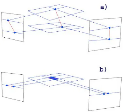
• point-like object (Figure 25a): we extract 2×2 image coordinates from the image pair, from which we can determine the 3-space coordinates of the object using a linear relationship;
• curve-like object (Figure 25b): we extract two curves from the image pair, each of which could be considered the “head-on” image of a projection surface extending in each field of view direction. The intersection of the two projection surfaces yields (in the ideal case) a unique 3-dimensional curve;
• surface-like object (Figure 25c): we can extract its visible edges from the image pair, but the respective projection surfaces refer to different locations on the surface to be reconstructed. This problem is underdetermined and without further information (for instance, the assumption of a surface curvature, the knowledge about the location of a light source, the surface reflectivity together with precise intensity measurements) a reconstruction is impossible.
Figure 25. Back projection to reconstruct point-like, curve-like and surface-like objects to illustrate the
For this reason in classical stereoscopy the edges, being curve-like objects, are reconstructed first.
In the next sections (3.2, 3.3 and 3.4) we describe the geometry relevant to stereoscopic observations (epipolar geometry) and the reconstruction‟s techniques (TP and LCT).
3.2 Epipolar Geometry
We have to find a suitable coordinate system so that the reconstruction can be reduced from a 3-dimensional to a set of 2-dimensional planar problems. For stereoscopy the geometrical conditions are such that two view points and two view directions are involved.
The line connecting the two view points is called the stereo base line, and subtends the stereo base angle between the two main view directions or optical axes of the respective telescopes (note that the two optical axes do not need to intersect). Let us take into account that the two observer positions and any object point to be reconstructed exactly define a plane. For many object points there will be many planes, but each of them will contain the two observer positions and is called epipolar plane (see Figure 26).
The projection of epipolar planes on both observer‟s images are lines (see Figure 26) and since any observer is on any epipolar plane, he sees them “head on”. These lines, called epipolar lines, generate a coordinate system on the image planes.
Moreover, depending on his field of view observer 1 may see observer 2 (and vice-versa), and since observer 2 is defined to lie on all epipolar planes, all epipolar lines in image 1 must converge in the projection of observer 2, called the epipole of the respective projection [Inhester, 2006].
Figure 26. Orientation of epipolar planes in space and the respective epipolar lines in the images for two
observers looking at the Sun. The observers telescope screens are derived from a projective geometry camera model (from Inhester, 2006).
Because the epipolar lines in one image depend on the position of both observers, any change in position of observer 2 requires a redetermination of epipolar lines also in image 1. The epipolar lines may be identified by the angle they form with a reference epipolar plane or by the coordinate of the plane‟s intersection with a suitable axis of a (completely independent) coordinate system, e.g., the z-axis in Figure 26.
In the STEREO context, the axis is the rotation axis of the Sun because, since the spacecraft are more or less close to the ecliptic, the Sun‟s rotation axis should intersect all relevant epipolar planes. With this choice, an epipolar plane is uniquely defined by the two observer‟s positions and its intersection point with the rotation axis.
Most space points lie on a unique epipolar plane, with the only exception of the points on the stereo base line. If these points are ruled out, any point which is identified on a certain epipolar line in one image must lie on the same epipolar line in the other image (epipolar constraint).
Figure 27. Virtual change of orientation of the observer‟s main view direction equivalent to
rectification. The rectified configuration is indicated by the rotated screens drawn in light blue (from Inhester, 2006).
We can therefore directly overplot the epipolar lines and their labels onto each image and thus determine the epipolar plane of an object from the image. As a consequence, we must only calculate the object‟s two-dimensional coordinates on the known epipolar plane, achievable from the measure of the positions of the object‟s projection along the epipolar line in either image.
The depth of an object results to be proportional to the difference of these coordinate values along the epipolar line of the two projections, the disparity. From the geometrical construction it results that epipolar lines usually are not parallel.
For an easy reconstruction it would be desirable to have the epipolar lines mapped into horizontal lines, this corresponding to the case when both spacecrafts have their optical axes directed parallel to each other (see Figure 27).
3.3 Tie-Point Reconstruction
As described above, we can reduce the reconstruction problem to a set of 2-dimensional problems. We segment each image densely into a (large) number of epipolar lines and compare the positions of a loop‟s intersections along the respective
Inhester [2006], showing how we can derive from these positions the intersection of the loop on the respective epipolar planes.
Let on a given epipolar plane the observer‟s positions be r1 and r2. For each epipolar plane we in addition specify a reference point r0 as the origin of the 2-dimensional coordinate system on this plane. For convenience, we take the intersection of the solar rotation axis with the epipolar plane the intercept of which could at the same time serve as a continuous label for the epipolar plane. For each observer we then introduce orthogonal coordinate axes vi and ei on the epipolar plane as shown in Figure 28: vi is the unit vector from the observer to r0 and ei is vi rotated clockwise by 90 degrees. Note that vi does not need to agree with the optical axis of the telescope nor must ei have the direction of the epipolar line.
We will take as rectified image coordinate along the respective epipolar line in image i the angle si between the direction to the object and vi. For convenience, we assume that the mapping of the observing telescopes can be described by a simple projective geometry camera model.
In this case, an object at an angular distance σ from the optical axis is mapped in the image to a distance ρ = f tan σ , where f is the camera‟s focal length.
Figure 28. Reconstruction of a point ∆r with projective (top) and affine (bottom) geometry (adapted
In this case, the angle si can be derived from the image distances ρ0 and ρ of the reference and object point‟s projection from the image centre, respectively, and their azimuth difference γ (see Figure 29) by:
(1) Here, the sign of si depends on whether the object is projected to the right (+) or left (-) of the line from the image centre to r0‟s projection. If there is any image distortion, the distances ρ0 and ρ read from the image have to be corrected accordingly.
Figure 29. Derivation of the angle s from the image coordinates for a projective geometry camera
model (from Inhester, 2006).
Formula (1) is numerically inconvenient for large focal lengths f and small image distances ρ. For ρ/f, ρ0/f → 0 relation (1) can be approximated by:
(2) which is the law of cosines applied to the triangle in the image plane in Figure 29. Hence, the angle s can in this limit be read directly from the image in units of arcsecs.
observers ri and either the reference point r0 or the two view directions vi to the reference point. In the latter case, r0 can be determined from (see Figure 28a):
(3) (4) Therefore a rectified image point (s1, s2) = (0,0) will have to be reconstructed at r0 and any other (s1, s2) pair will be conveniently expressed as a 2-dimensional distance vector ∆r from r0.
For affine geometry, all view directions from an image i are approximated to be parallel to vi. Then (see Figure 28b):
(5) If we subtract the two above lines we obtain the “depth” component of ∆r in direction half way between the two view directions. Note, with beta the angle between
v1 and v2 we have v1 + v2 = (e2 − e1)/tan(β/2). Then:
(6) where the difference on the right hand side is the disparity. In the simplest case, the depth of an object is directly proportional to the disparity of its projections along the epipolar lines.
Figure 30. Reconstruction of a curve segment (red) with different inclination with respect to the
adjacent epipolar planes (blue). In the top drawing the line segment in inclined to, in the bottom drawing it lies exactly on an epipolar plane (adapted from Inhester, 2006).
For projective geometry we take account of the divergence of the view directions emerging from each observer. The angle si between the reference point r0 and an object in the epipolar plane then is (see Figure 28a):
or
(7) in contrast to (5). To justify the more simple affine geometry formula, s1 and s2 must both be small.
For EUVI images, s is of the order of the apparent solar disk radius of about 0.005 radian. For HI images, however, with a much larger field of view, projective geometry
eigenvalue considerably. The eigenvalue of a matrix (a, b) is O(|a × b|) if it is small compared to |a| and |b|. Hence if the view directions are nearly parallel, the difference between affine and projective geometry may be non-negligible even if s is small. For each epipolar plane we obtain a set of intersection points and all we have to do is to connect the intersection points between neighbouring planes to obtain 3-dimensional curves. This last step involves some uncertainties if different loops come close. To obey the disparity continuity constraint we should keep track of the intersections across the epipolar planes by reconstructing curve segments between epipolar lines rather than only points on single epipolar lines (practically, we just combine the intersection points of a given curve projection with epipolar lines to ordered lists). Hence the method should better be called tie-curve rather than tie-point method.
The curve segments from each image are then projected along their respective geometrical view direction (either affine or projective) which yields a narrow planar strip of the projection surface of the curve (see Figure 30a). The intersection of the strips from both images gives a small line segment of finite length, the end points of which are two points of the three-dimensional loop curve. The intersection is guaranteed since the curve sections in the image were chosen from the same epipolar interval.
This strategy runs into a problem, however, if the curve segment is directed parallel to an epipolar line (see Figure 30b). The geometrical intersection of the two projection ribbons now is not a line segment anymore but a small trapezoid. This object of dimension 2 is difficult to incorporate to our final 3D loop curve of dimension 1. This problem, however, is not a deficit of the method but a fundamental geometrical limitation.
3.4 Local Correlation Tracking (LCT)
Another technique utilized in stereoscopy is the local correlation tracking [Mierla et al, 2009].
To find the correspondence between the images, i.e., to identify the same pixels
appearing in both images, is one of the key problems of stereoscopic reconstructions. Unfortunately, CMEs often have a rather diffuse density distribution where prominent,
well-located points are difficult to identify. Instead of using a feature-based correspondence, we should use a correlation-based approach (see, e.g., Trucco and Verri, 1998). In such a correlation-based method the elements to be matched are small sub-images of fixed size, called “match windows”. The criterion which decides whether two such windows in each image are positioned on the same object is their mutual correlation coefficient.
In order to find correlations, we keep the match window in a fixed position on a given epipolar line in one image and move it along the same epipolar line in the other image. If a maximum of the correlation occurs at a certain shift, the center position of the windows is used for tie-pointing the 3D region which has probably produced this high correlation. This procedure is subject to some constraints in order to catch meaningful correlations and discard improbable ones. First we use normalized cross-correlations on the match windows W:
(8)
with σAB ∈ [−1, 1]; where IA(x, y) and IB(x, y) are the respective intensities after rectification at positions given by the epipolar line coordinate y and the horizontal
coordinate x. The integrals are done over the whole pixels in the window W (ξ and ζ). This choice is sensitive also to correlations at low intensity levels. In order to discard
spurious correlations, we limit the maximum disparity |x – x‟|. Since the disparity for a given spacecraft configuration is directly proportional to the reconstructed depth, this limitation is equivalent to restricting the reconstructed CME to a certain depth range. The depth is defined as the distance of a feature from the plane of the sky. The shift limits are set so that a depth range of ±5R⊙ (corresponding to COR1 data) and ±12 R⊙ (corresponding to COR2 data) resulted. Finally, only maxima of σAB(x, x‟, y) > 0.9 are
For this method we use the total brightness (tB) images because the tB scattering cross section is isotropic within a factor of two. The decrease of the scattering function away from the plane of the sky is essentially due to the 1/r2 decrease of the primary solar radiation. Note that the normalization in correlation (8) takes care of a possibly different signal intensity of a given structure in the two images.
3.5 Coordinate System and Display of 3D Features
All our reconstructions of halo CMEs shall be displayed in the same coordinate system for easy comparison. We choose the Heliocentric Earth Equatorial (HEEQ) coordinate system for this purpose [Hapgood 1992]. It has its origin at the Sun‟s center, the Z is the solar rotation axis, X is in the plane containing the Z-axis and Earth, at the intersection of the solar central meridian and the heliographic equator, and Y completes the right-handed coordinate system.
We also use Stonyhurst heliographic coordinates (Figure 31) which are closely related to HEEQ coordinates [Thompson, 2006].
Figure 31. A diagram of the Sun, showing lines of constant Stonyhurst heliographic longitude (Φ) and
latitude (Θ) on the solar disk. The origin of the coordinate system is at the intersection of the solar equator and the (terrestrial) observer‟s central meridian. This representation is also known as a
The coordinates are represented in the spherical coordinate system as latitude, longitude, and distance from the Sun‟s center. The value of the longitude ranges between −180° and +180°. This also means that the front side disk longitude ranges between −90° and +90°. The image coordinates are given by the X-axis and the Y-axis.
In order to display the reconstructed points, we use the following procedure. The resulting 3D positions are displayed as isodensity surfaces. In a given geometry, the space around the Sun is divided into a rectangular grid, and the density is calculated for each cell (voxel8). The resolution of the reconstruction depends of the cell size (for our data we use a cube of 256×256×256 cells).
In what follows, we apply the mentioned techniques to the SECCHI-COR data, in order to reconstruct the CMEs and/or their directions of propagation. We make use of the local correlation tracking (LCT) to identify the same feature in COR Ahead and COR Behind images. Then, using tie-point (TP) reconstruction method we infer the 3D structure of CMEs. We refer to this as the LCT-TP reconstruction technique. These techniques are applied on three structured CMEs9 observed by COR1 and COR2 instruments on 3 April 2010, 7 August 2010 and 15 February 2011 (see Section 4). The objects we deal with here are localized blobs of plasma that we can discriminate in a CME cloud. The selection of the features to be tracked is based on the fact that they were easily and unambiguously identifiable by naked eye in both A and B images. Because these features are part of the global CMEs, their selection will not affect our results regarding the determination of the direction of propagation of the CME. The blobs are often still diffuse and cannot be localized to high precision compared to, for example, loops in EUV images. For this reason, we argue that it is justified to relax the reconstruction constraints slightly.
For this study we assume that a) the two spacecrafts are in the ecliptic plane (i.e., the STEREO mission plane and the ecliptic are approximately the same) and b) we can
8 A voxel (volumetric pixel or Volumetric Picture Element) is a volume element, representing a value on a regular grid in three dimensional space. This is analogous to a pixel, which represents 2D image data
use affine geometry10 for the reconstruction instead of projective geometry. As a consequence, we can treat epipolar planes in each image as being parallel to the ecliptic.
The geometric localization tool consists of IDL (Interactive Data Language) programs that can process SECCHI COR images. Based on the time period of interest provided by the user, the programs retrieves, processes, and displays a pair of concurrent coronagraph images taken by SECCHI-A and SECCHI-B.
The images of the CMEs events are stored on the computer in the fits (Flexible Image Transport System) file format. Then manually we selected the CME‟edge from each image. User intervention is necessary at this point because of the difficulty in automatically identifying the faint boundary of the CME as a whole, instead of the sharper edges associated with bright coronal features, such as, for example, streamer belts or structures internal to the CME.
Once that we have identified the region of interest from each of the two images, the geometric localization tool automatically applies several coordinate transformations. These transformations include corrections for projection effects applied to the raw pixel positions within the region of interest, using some IDL SolarSoft routine.
10 The use of affine geometry is justified since the objects that are to be reconstructed are typically 200 R⊙ away from the observer. This distance is much greater than the typical size of the objects/features and their distance from the Sun. Affine geometry assumes the observer is located at an infinite distance, such that different viewing angles can be considered parallel, and objects near the Sun appear the same size independent of their distance from the plane of the sky.