https://doi.org/10.1177/0959683617714596 The Holocene
2018, Vol. 28(1) 56 –64 © The Author(s) 2017 Reprints and permissions:
sagepub.co.uk/journalsPermissions.nav DOI: 10.1177/0959683617714596 journals.sagepub.com/home/hol
Introduction
The impact of sea-level rise is one of the main concerns related to ongoing global warming, and our capacity to estimate the regional-to-local impact on the coast environment relies on the assumption that many local variables are known (e.g. eustatic sea-level component, tectonic uplift, subsidence and glacial isostatic adjustment; Alley et al., 2005; Blum and Roberts, 2009; Lambeck et al., 2014; Milne et al., 2009; PALeo SEA Level Working Group (PALSEA), 2009). In this framework, the reconstruction of the relative sea-level (RSL) changes at regional scale during the Holocene is particularly relevant and the accuracy of its estima-tion is crucial for testing geophysical models (Milne and Mitro-vica, 2008).
With its 2000 km of coast, the Atlantic Patagonian passive margin represents a natural link for exploring the RSL evolution between ‘near’ and ‘far’ field sites (Milne et al., 2005; Rostami et al., 2000). Therefore, this is a strategic area in which to focus palaeo sea-level studies (Codignotto et al., 1992; Isla and Angulo, 2015; Milne et al., 2005; Pedoja et al., 2011; Ribolini et al., 2011; Rostami et al., 2000; Rutter et al., 1989, 1990; Schellmann and Radtke, 2000, 2003, 2010; Zanchetta et al., 2014). However, a precise and accurate estimation of the RSL in this area has been complicated by several factors, namely (1) precise and accurate sea-level indicators such as notches, inner terrace margins, coral reefs and algal encrustations have been rarely used or not found
(Bini et al., 2013, 2014; Pedoja et al., 2011; Ribolini et al., 2011); (2) sea-level indicators have generally been measured using a barometric altimeter or graduate bars equipped with spirit level, starting from the local high-tide level implying a wide vertical error up to ±3 m (Zanchetta et al., 2012, 2014); and (3) the coastal area is within the macro-tidal regime (Isla and Bujalesky, 2008) and is characterized by high hydrodynamic regimes, so that most of the sea-level indicators are related to surf and storm extension rather than to mean sea level. As a consequence, Schellmann and
Mid-Holocene relative sea-level changes
along Atlantic Patagonia: New data from
Camarones, Chubut, Argentina
Monica Bini,
1,2Ilaria Isola,
2,3Giovanni Zanchetta,
1,2Marta Pappalardo,
1Adriano Ribolini,
1Luca Ragaini,
1Carlo Baroni,
1,3Gabriella Boretto,
4Enrique Fuck,
5Caterina Morigi,
1Maria Cristina Salvatore,
1,3Davide Bassi,
6Fabio Marzaioli
7and Filippo Terrasi
7Abstract
This paper concerns the relative sea-level changes associated with the Atlantic Patagonian coast derived from sea-level index points whose elevation was determined by a differential global position system (DGPS). Bioencrustations from outcrops located near Camarones, Chubut, Argentina, consist of autochthonous deposits characterized by Austromegabalanus psittacus (Molina, 1782), encrusting acervulinid foraminifera, coralline red algae and bryozoans. The association of the different organisms is interpreted as being associated with an intertidal environment, and they have been used as index points to establish the relative sea-level position. The main conclusion is that the relative sea-level between c. 7000 and 5300 cal. yr BP was in the range of
c. 2–4 m a.s.l., with a mean value of c. 3.5 m a.s.l. Our data seem to support the existence of different rates of relative sea-level fall in different sectors of
Atlantic Patagonia during the Holocene and highlight the importance of a more precise and accurate relative sea-level estimation by producing new data and revisiting the indicative meaning of most of the indicators so far used in the area.
Keywords
Atlantic Patagonia, biological markers, Holocene, relative sea level Received 22 July 2016; revised manuscript accepted 14 April 2017
1Dipartimento di Scienze della Terra, Pisa University, Italy 2Istituto Nazionale di Geofisica e Vulcanologia, Pisa, Roma, Italy 3 CNR-IGG, Consiglio Nazionale delle Ricerche, Istituto di Geoscienze e
Georisorse, Italy
4 CICTERRA-CONICET Centro de Investigaciones en Ciencias de la
Tierra, Universidad Nacional de Córdoba, Argentina
5 Facultad de Ciencias Naturales y Museo, Universidad Nacional de La
Plata, Argentina
6Dipartimento di Fisica e Scienze della Terra, Università di Ferrara, Italy 7 CIRCE, Department of Mathematics and Physics, Second University of
Naples, Italy
Corresponding author:
Monica Bini, Dipartimento di Scienze della Terra, Via S. Maria 53, 56126 Pisa, Italy.
Email: [email protected]
714596HOL0010.1177/0959683617714596The HoloceneBini et al.
research-article2017
Radtke (2010) and Zanchetta et al. (2014) reported a different alti-tudinal estimation for the Holocene RSL, using different indica-tors related to coastal sediments (i.e. beach ridges and littoral terraces). Some authors take a different approach in measuring reference sea level (e.g. top vs base of beach ridges; Pappalardo et al., 2015), complicating the use of reported data (Codignotto et al., 1992; Pedoja et al., 2011; Ribolini et al., 2011; Rutter et al., 1989, 1990), while others report data related to high-tide level (Schellmann and Radtke, 2010, and references therein, Zanchetta et al., 2012, 2014). The correlation between elevation values mea-sured above high tide and values meamea-sured above mean sea level is not so straightforward, and regional correlations are compli-cated. Although the data from this vast region would be of para-mount importance, recent geophysical modelling of sea-level change along the South American coast has not accounted for the Patagonian data (Milne et al., 2005), presumably because of their very high level of uncertainty.
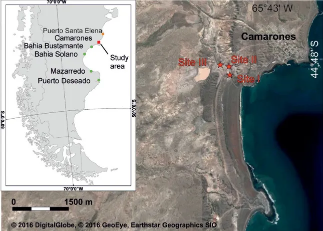
In this paper, we report on a RSL reconstruction based on in situ fossil barnacles and foraminiferal–bryozoan concretions. These sea-level indicators have never been described along the Patagonian coast so far. Here, we describe the indicators found in the territory of Camarones (Chubut, Argentina, Figure 1), one of the nodal areas for the reconstruction of the RSL oscilla-tions along the Patagonian coast owing to its abundance of raised beaches with datable materials (Pappalardo et al., 2015; Schellmann and Radtke, 2010; Zanchetta et al., 2012). More-over, the elevation of the indicators was for the first time mea-sured by a DGPS, which provided reliable sea-level values at an accuracy never previously reached along the Patagonian coast. Finally, we standardized our data in terms of sea-level index and limiting points (e.g. Rovere et al., 2016; Shennan et al., 2015; Vacchi et al., 2016). This approach, totally new for the Patagonian coast, is mandatory for future regional and extra-regional correlations.
The study area
The study area is located in the southern part of the Bahía Cama-rones, Chubut (Argentina), c. 40-km-wide gulf extending from c. 44°54′S to 44°34′S (Figure 1). Structurally, the area is located on the southern edge of the so-called North Patagonia Massif (Ferug-lio, 1950). Mostly, Jurassic volcanic rocks formed the pre-Quater-nary succession (Marifill Formation; Lema et al., 2001). Inland morphology is characterized by flat surfaces covered by Late Neogene–Early Quaternary fluvial gravelly deposits (‘rodados
Patagonicos’ in Martinez and Coronato, 2008), while the
land-scape is dominated by Quaternary littoral and continental deposits raised at various elevations close to the coast (Lema et al., 2001; Pappalardo et al., 2015).
Like most of coastal Patagonia, the area is dominated by high-energy, macro-tidal and stormy conditions (Isla and Bujalesky, 2008), resulting in a coastal morphology dominated by cliffs, shore platforms and coarse-clastic beach ridges (‘swash built ridges’ sensu Tanner, 1995).
In Camarones, the predictions of the astronomic tide eleva-tions are calculated in relation to the harbour of Puerto Santa Elena (Figure 1) according to the data released by the Servicio de Hidrografìa Naval (http://www.hidro.gov.ar). For the area of Camarones, the maximum tidal range is c. 5 m, while the mean is
c. 3.5 m (Figure 2).
Most of the studies on Holocene coastal evolution are concen-trated in the southern part of the Bahía Camarones area and pro-vide a robust chronological constraint for coastal aggradation during the Holocene (Codignotto et al., 1992; Schellmann, 1998; Schellmann and Radtke, 2000, 2003, 2010). In total, two evolu-tionary phases have been distinguished: (1) the first phase, the maximum Holocene ingression (c. 6.8–6.5 kyr BP), is character-ized by the formation of littoral and estuarine deposits (Schell-mann and Radtke, 2010) found at the sea embayment along local creeks (locally named ‘cañadon’); (2) the successive phase, still
Figure 1. Location map of the studied area.
58 The Holocene 28(1)
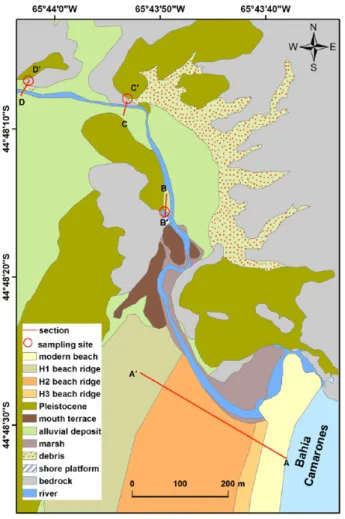
active, is marked by discontinuous coastal aggradation, with the formation of prominent higher gravelly beach ridges parallel to the present-day coast (Figure 3).
Methodology
For stratigraphic and geomorphological investigations, we fol-lowed the same approach already used in previous studies con-ducted in the area (Isola et al., 2011; Ribolini et al., 2011). A preliminary remote sensing analysis was performed using LAND-SAT 7 images (acquisition dates, 1999–2001) and Quick Bird
images (acquisition date, 2004) supported by the digital elevation model Shuttle Radar Topography Mission (SRTM; https://www. jpl.nasa.gov/srtm). After this preliminary phase, field surveys were carried out in February 2009, 2010 and 2011 (Pappalardo et al., 2015; Zanchetta et al., 2012). In the first phase, the eleva-tion data were obtained using graduate bars equipped with spirit level, starting the measurements from the nearest Instituto Geográfico Nacional point (IGN), with a precision in the order of ±0.3 m (Zanchetta et al., 2014). A field survey conducted in Janu-ary 2016 was dedicated to the DGPS measurement of sea-level indicators. The data were acquired by the WGS84 Geographic Coordinate System (maximum error in elevation of acquired points was 10 cm) and post-processed and referred to the current global geoid model EGM2008 (Pavlis et al., 2012; 4 cm planimet-ric error and 9 cm elevation error). Elevation measurements indi-cated as ‘a.s.l.’ in this paper are referred to the vertical datum EGM2008. These data integrate and basically confirm those pre-viously obtained by graduated bar measurement. For the study area, Schellmann and Radtke (2010) reported the altitudinal mea-surement of different sea-level indicators, using a barometric altimeter (reported precision ±1 m) daily calibrated with the tide level. In order to compare our data with those reported by Schell-mann and Radtke (2010), we used the DGPS to re-measure some of the sections described by Schellmann and Radtke (2010).
In situ barnacles and encrusting foraminiferal deposits were col-lected in the field and measured with DGPS (Figures 1 and 3), alongside additional samples with articulated valves of Mytilus
edu-lis from littoral deposits. The samples for radiocarbon dating were
cleaned in an ultrasonic bath with the addition of oxygen peroxide and then gently etched with diluted HCl to remove any recent car-bonate encrustation. Radiocarbon measurement was carried out at the CIRCE laboratory of Caserta, Italy (Terrasi et al., 2007, 2008) and calibrated using the Marine13 curve (Reimer et al., 2015). How-ever, the reservoir effect values for the Southern Atlantic Ocean and, in particular, Patagonia, are not well constrained (Schellmann and Radtke, 2010). Specific studies suggest that for different localities of the Patagonian coast between c. 42°S and 50°S, the reservoir effect can vary between 180 and 530 years (Butzin et al., 2005; Cordero et al., 2003; Schellmann and Radtke, 2010).
Collected species, radiocarbon dates and sampling site eleva-tion are reported in Table 1. The state of preservaeleva-tion of barnacles and encrustations, prior to dating were assessed by stereomicro-scope analysis of thin sections and was investigated by x-ray power diffraction (XRD).
Results
The study area is located along a small river to the south of the Camarones village (Figure 1). A succession of
Figure 2. Tide level derived from the current tide tables of Puerto Santa Elena. Elevation data are referred to the reduction plane (theoretical
plane located under the mean sea level in order to have only positive tidal values in the tables).
MLLW: mean lower low water; MLHW: mean lower high water; MHLW: mean higher low water; MHHW: mean higher high water; MHW: mean high water; MTL: mean tide level.
Figure 3. Simplified geomorphological map of the studied area.
H: Holocene beach ridges subdivided into H1, H2 and H3 from the old-est to the youngold-est beach ridge, according to the morphostratigraphic units identified by Schellmann and Radtke (2010); P: Pleistocene beach ridge.
Holocene–Pleistocene gravelly beach ridges forms the coastal strandplain, up to a distance of >500 m inland from the present coastline. This arched beach ridge system is incised by a river val-ley where alluvial, marsh and coastal sediments were deposited (Figures 3 and 4a). Along the river valley, bedrock crops out form-ing steep cliffs in some places and relict shore platforms locally. In total, three rocky outcrops, composed by welded ignimbrites of Marifil Formation, yielded barnacles (A. psittacus; Molina, 1782) and foraminiferal encrustations (mostly Acervulina inhaerens; Schulthe, 1854) in life position (Figures 3, 4b–d, 5 and 6). The first outcrop (Figures 3 and 4b) is formed by a vertical cliff exposed for
c. 3–4 m and a flat top surface, located at c. 5 m a.s.l., representing
the remnant of a shore platform. Barnacles and foraminiferal encrustations are located on the cliff where barnacles are discon-tinuously spread for <1 m (between 3.4 and 3.8 m a.s.l.) and encrus-tations for c. 1.5 m (between 3.3 and 4.8 m a.s.l.; Figures 4b and 5). The second outcrop (Figures 3, 4c and 5) is formed similarly by a vertical cliff with an on-top shore platform covered by gravelly deposits. On the vertical cliff barnacles span between 3.1 and 3.9 m a.s.l. and incrustations from 3.3 to 4.6 m a.s.l. The third sampled
inland site is represented by boulders at the toe of a rocky cliff (Figures 3, 4d and 5). Barnacles and incrustations, spanning in elevation between 3.2 and 4.2 m a.s.l., developed on the blocks and at the base of the cliff.
In each sampled site, barnacles (A. psittacus) occur as isolated or two to three jointed individuals (Figure 6). Most of the encrus-tations consist of foraminifera identifiable as Acervulina
inhae-rens (Figure 6d–f), which is the dominant component, while
arborescent forms such as Homotrema and Miniacina are less frequent. All these encrusting foraminifera form repetitive or ran-domly arranged inner superimposed growth stages. Superim-posed growth stage bryozoans and rare coralline red algal thalli occur within the A. inhaerens. The bryozoans are represented by encrusting cheilostomes (Anascina?), and the very low preserva-tion does not allow their systematic identificapreserva-tion. The corallines are almost micritized and/or recrystallized. A possible uniporate conceptacle was also identified. This reproductive character along with the vegetative characters (cell fusions and monomerous cell filaments) suggests a possible ascription to the Mastophoroideae subfamily (Figure 6d–f).
Table 1. Radiocarbon ages obtained for this study were performed using IntCal13 and Marine13 radiocarbon age calibration curves (Reimer
et al., 2015).
Laboratory code Sample code 14C yr BP Cal. yr BP (±2σ) Material Elevation (m a.s.l.)
DSH2744 Wpi-424-2 5641 ± 46 5924–6168 Australomegabalanus psittacus 3.7 DSH3170 Wpi-436A 5515 ± 50 5741–6015 Australomegabalanus. psittacus 3.6 DSH2738 AO-164 5132 ± 67 5313–5608 Australomegabalanus psittacus 3.9 DSH2742 Wpi-436b 4995 ± 89 5106–5560 Encrustation 3.6 DSH2736 AO-154D 5567 ± 44 5865–6099 Mytilus. edulis 3.9 DSH2745 Wpi-436 5562 ± 43 5861–6092 Mytilus edulis 5.2 DSH4023 AO-164 5370 ± 60 5604–5878 Mytilus edulis 3.5 Hd-23504 Pa04/7a 5560 ± 38 5866–6065 Protothaca antiqua 3.8 aData from Schellmann and Radtke (2010).
Figure 4. Geological sections (see map in Figure 2 for location): (a) geological section AA′, (b) geological section BB′, (c) geological section
60 The Holocene 28(1)
The top surface of the first outcrops is carved in a previously modelled rocky terrace attributed by Schellmann and Radtke (2010) to marine isotope stage 7 (MIS 7). A shell accumulation of
M. edulis rests directly on the lateral margin of the lower shore
platform, sealed by a few decimetre-thick slope deposits. No other deposits cover the shore platform. This shell accumulation, with a poor sandy matrix of some millimetre-size rounded clasts, and some shells with valves still joined, is consistent with a storm deposit. One shell from the accumulation yielded a radiocarbon age of 5562 ± 43 yr BP. Concretion from the vertical cliff of this
outcrop yielded a radiocarbon age of 4995 ± 89 yr BP, whereas one barnacle yielded 5515 ± 50 yr BP.
The top surface of the second rocky outcrop is covered by gravelly deposits, which did not yield suitable material for dating (i.e. only fragmented shells and not entire shells with articulated valves). However, these deposits are reasonably related to the formation of the Holocene erosional platform. In the vertical cliff of this second outcrop, a barnacle yielded a radiocarbon age of 5132 ± 67 yr BP. Here, the rocky cliff was crossed by some vertical fissures containing sediment and some fossil remains, including M. edulis and barnacles (Figure 6c). One sample with articulated valves of M. edulis collected from the infilling of the vertical fissures yielded a radiocarbon age of 5567 ± 44 yr BP. On the third site, a sample of barnacles revealed a radiocarbon age of 5641 ± 46 yr BP.
All the rocky cliffs are partially sealed by gravelly estuarine ter-raced deposits, namely, valley-mouth terraces, according to Schell-man and Radtke (2010, Figure 3). These deposits contain shells (principally Prothotaca antiqua and M. edulis) accumulated in lenses for which Schellman and Radtke (2010) reported a radiocar-bon age of 5560 ± 38 yr BP. A new radiocarradiocar-bon measurement was undertaken on an M. edulis from the same deposits, directly sealing the second cliff, yielding a consistent age of 5370 ± 60 yr BP.
Figure 5. Elevation range of barnacles and incrustations in the
three outcrops described. The data were measured by DGPS Trimble with a maximum error of 10 cm in elevation.
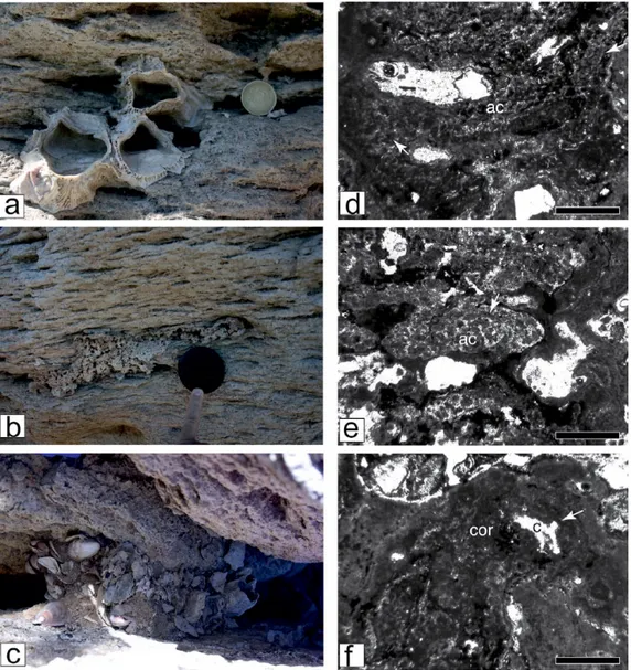
Figure 6. Images of (a) barnacles (Austromegabalanus psittacus), (b) incrustation, and (c) storm deposit infilling fractures within bedrock.
Thin-section microscope photographs of the studied bioencrustations. (d, e) Encrusting acervulind shells (ac) showing chamber arrangement (arrows) with successive layers in sub-axial sections; the chambers are open in lateral walls (arrows); (f) encrusting coralline algal thallus (cor) showing the transversal section of a uniporate conceptacle (c) with a cylindrical porecanal (arrow). Scale bar represents 500 µm.
Discussion
Sea-level indicators in Atlantic Patagonia have yielded controver-sial results in the estimation of past RSL, and their accuracy and precision have been poorly defined, both for the precision of the measurement of the method applied (barometric altimeter, local maps and graduate bars) and for the unclear meaning of the indi-cators, for example, storm and maximum high tide (Codignotto et al., 1992). Therefore, it is mandatory to transform sea-level indicators into index or limiting points to improve RSL estima-tions (Shennan et al., 2015). So far, the most precise and accurate indicators described for Atlantic Patagonia, which can be easily transformed into sea-level index points, are the erosive notches. Specifically, the retreat point of notch defines the main high-tide values (±0.3 m; Bini et al., 2014).
The Camarones association of barnacles, bryozoans and encrusting foraminifera can be generically interpreted as inter-tidal–subtidal indicator (e.g. Baker et al., 2001; Ferranti et al., 2006; Laborel and Laborel-Deguen, 1994; Pirazzoli et al., 1985; Rovere et al., 2015, 2016).
Specifically, the collected samples of barnacle correspond to the ‘acorn barnacle’ A. psittacus (Figure 6a), a species inhabiting mainly rocky substrates of the subtidal zone, where it forms dense aggregates between 5 and 7 m in water depth (López et al., 2010). However, the functional faculties of the barnacle could account for the high capacity of A. psittacus to also colonize habitats exposed to prolonged emersion periods like those char-acterizing intertidal settings (López et al., 2003). The barnacles generally live in groups forming dense hummocks but in less favourable locations like the intertidal zones where they are less frequent and distant from each other. The relatively sparse asso-ciation of barnacles in our sampling sites indicates the upper limit of the living range.
Present-day acervulinid foraminifera show a large bathymetric range from the intertidal zone down to 100 m in water depth (Bassi et al., 2012; Perry and Hepburn, 2008). Although acervuli-nids are more common in deeper water settings where interspe-cific competition for space may be reduced (Rasser and Piller, 1997), Acervulina inharens thrives in shallow water Bahamas shelf settings (<30 m; Walker et al., 2011). Homotrema is reported
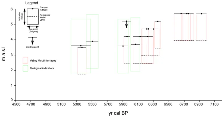
from high-energy shallow water settings (Gischler and Möder, 2009). So far, Homotrema has seemed to be an excellent indicator of high-energy water conditions for shallow near-shore and shelf/ edge habitats, where water energy during tidal exchange is greater in tropical and subtropical environments (Walker et al., 2011), and even in this case, it is consistent with the intertidal zone. Moreover, it is generally assumed that fossil barnacles and bio-encrustation in growth positions are easily eroded (Pirazzoli et al., 1985). Therefore, the survival of encrusted shell remains at higher-than-present levels suggests a sea-level fall sufficiently rapid for the shell to escape obliteration by wave erosion (Piraz-zoli et al., 1985), a condition favouring the preservation of species that live in the upper limit of the high tide. In most cases, the age of the outer shells on a thick vertical encrustation will correspond to the terminal period of the former sea-level stand (Baker et al., 2001). Therefore, the Camarones barnacles, bryozoans and encrusting foraminifera association can be considered substan-tially intertidal, and its definition of index point could be possible on the basis of tide oscillations (Shennan et al., 2015; Vacchi et al., 2016). By assuming that our association is strictly intertidal between c. 6100 and c. 5300 cal. yr BP RSL was around 3.7 and 3.9 m a.s.l. (Figure 7).
For the studied area, Schellmann and Radtke (2010) reported several radiocarbon measurements for different sea-level indica-tors, which can complete and improve the interpretation of the data discussed in this paper. In our study, we selected only the valley-mouth terrace sea-level indicators, which are less affected by storm deposition, compared with beach ridges, thus reducing the errors in elevation estimation (Schellmann and Radtke, 2010; Tamura, 2012; Zanchetta et al., 2014). According to the observa-tions of modern analogs by Schellmann and Radtke (2010), val-ley-mouth terraces are estuarine deposits that contain lateral/ vertical interfingering of mollusc-bearing littoral sediments and fluvial deposits forming at the mouth of small local rivers. The top of the valley-mouth terraces correlates directly to the former elevation of the high-tide level representing a suitable indicator to be used as index point. As can be inferred from Figure 7, RSL from mouth terraces is consistent within the indicative meaning of barnacles and encrustations supporting our interpretation.
Figure 7. Total plot of the Camarones area index points: fixed biological indicators from this work; valley-mouth terrace indicators from
62 The Holocene 28(1)
Indeed, at least three of our biological indicators, chronologically overlapping the data from valley-mouth terraces, lie within 1 m of the top of the mouth terraces. Significantly, the presence of the storm deposit dated c. 5950 cal. yr BP, located directly on the erosive shore platform on top of the first cliff, represents an upper RSL limiting point (Figure 7), constraining fairly well the values of fossil barnacles and mouth terrace. The storm deposit can also be considered a termine ante quem for the formation of the rock platform on top of the first outcrop.
Considering the elevation of the index points obtained from mouth terraces in the area together with the biological indicators discussed in this paper, this evidence collectively (Figure 7) agrees on indicating the RSL to be from c. 2 to c. 4 m a.s.l. between c. 5300 and 7000 cal. yr BP.
In Figure 7, the altimetric and chronological data of the valley-mouth terraces show a highstand between c. 7000 and 6600 cal. yr BP at c. 4 m a.s.l., followed by a progressive fall to c. 2–2.5 m between 6200 and 5300 cal. yr BP. The radiocarbon age of the storm deposit above the shore platform may indicate that this shore platform was related to the higher sea stand at c. 7000 cal. yr BP and was no longer significantly active during the progres-sive fall after c. 6200 cal. yr BP, only occasionally reached by storms. However, the RSL variation recorded by the valley-mouth terraces is not shown by barnacles and encrustation, thus suggest-ing that most of this variation falls within the range of error of the two index points.
Following Shennan and Horton (2002), the total vertical error (including vertical distribution of encrustation and barnacles, Fig-ure 5; measFig-urement errors and indicative meaning) for the bio-logical sea-level indicators is c. 3.8 m. According to Schellman and Radtke (2010), a minimum vertical error for valley-mouth terraces can be calculated at c. 2 m. However, a precise estimation of error should be associated with an accurate review of modern analogs on the valley-mouth terraces and of other findings from fixed biological indicators. Overall, the mean RSL between c. 7000 and 5300 cal. yr BP, which can be obtained considering all the index points, is 3.4 ± 0.6 m a.s.l.
Initial glacio-hydro-isostatic models of the Patagonian coast suggested that the shoreline could be characterized by currently raised beaches, which started to form as soon as ice-sheet melting ceased (Clark et al., 1978). A more recent model (Milne and Mitro-vica, 2008) predicted that RSLs might have exceeded present by c. 5 m at 6000 cal. yr BP. Field evidence indicates that the highstand is somewhat c. 1.5 m lower than model prediction. These ranges of measurement can agree with the model considering all the vertical errors associated with the index points discussed.
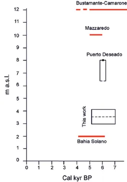
A comparison of the different sectors of the Atlantic Patago-nian coast is complicated by many factors. Codignotto et al. (1992) found a significant rate of RSL changes during the Holo-cene in relation to different tectonic sectors. They indicated a maximum highstand at c. 12 m a.s.l. for the period c. 4–8 kyr BP for the area of Camarones–Bustamante, at c. 2 m a.s.l. for the period c. 4–6 kyr BP in the area of Bahia Solano (Figure 8). These data are affected by poor quality radiocarbon dating together with low altimetric accuracy. Moreover, most data are obtained by measuring the altitudinal crest of beach ridges, which are largely affected by storm conditions (Schellmann and Radtke, 2010; Tamura, 2012; Zanchetta et al., 2014). On the contrary, Schell-mann and Radtke (2010) observed no appreciable differences along the Patagonia coast. However, using different sea-level indicators, the authors observed different values (reported above high tide (a.h.T)) for the highstand, occurring between c. 6 and 7 cal. kyr BP, ranging from c. 9 to 5 m a.h.T. Bini et al. (2013, 2014) and Zanchetta et al. (2014) reported an RSL at c. 8 m a.s.l. at c. 3500 cal. yr BP by accurate measurements of erosive notches in the Puerto Deseado area (Figure 1). Owing to the difficulty in dat-ing erosive notches, Zanchetta et al. (2014) suggested that these
notches were formed during a previous Holocene highstand. In any case, the RSL marked by well-preserved notches is higher than that observed in the Camarones area, indicating that a differ-ent RSL may exist along the Patagonian coast during the same period (Figure 8).
In this respect, Pedoja et al. (2011) suggested that the presence of the Nazca and the Antarctic plates subducting under South America and southern Patagonian, respectively (Ramos and Ghi-glione, 2008, and references therein), may have produced a long wavelength tectonic effect, onto which the glacio-hydro-isostatic signal is overprinted. This signal can vary according to the differ-ent sectors of the Atlantic Patagonian coast. More recdiffer-ently, Isla and Angulo (2015) in an accurate review of existing data from MIS5 terraces along Atlantic Patagonia have shown the impor-tance of the effect of subduing plates in determining regional trends in the rate of uplift. The data discussed in our paper seem to support the possible existence of a different uplift rate over the Atlantic Patagonian coast. However, subtle differences can only be identified by appropriate markers and are probably difficult to identify using the data so far available, which are affected by large measurement uncertainty and incomplete understanding of the indicator meaning.
Conclusion
We have presented the first accurate middle-Holocene RSL deter-mination for a well-dated period of time using different sea-level indicators, for the Atlantic Patagonian coast, with altitudinal mea-surement obtained using DGPS. Once dated, and their meaning and vertical error discussed, the indicators were transformed into index points. In this paper, using the available evidences, we sug-gest that the in situ association of sparse barnacles, bryozoans and encrusting foraminifera can have the indicative meaning of inter-tidal indicators, in the absence of modern analogs for the area. The mean RSL was estimated at c. 3.50 m a.s.l., lower than the c. 5 m predicted by the global model, using estuarine deposits (i.e.
Figure 8. Relative sea-level (RSL) data along the Patagonian
coast for the ‘highstand’ by different authors: redline: data from Codignotto et al. (1992); dark line: data from Zanchetta et al. (2014) and from this work reported as a.s.l. (for sites location, see Figure 1). The indicative meaning reported in this figure is discussed in the text, while the indicative meaning cannot be reported for Codignotto et al. (1992).
mouth terraces) together with barnacles, bryozoans and encrust-ing foraminifera, for the period comprised between c. 5300 and 7000 cal. yr BP (Milne and Mitrovica, 2008).
Regional considerations indicating that the existence of differ-ent rates of RSL falls in differdiffer-ent sectors of Atlantic Patagonia, as reported in the past by Codignotto et al. (1992) and refuted by recent works (Schellmann and Radtke, 2010), need to be recon-sidered. In this framework, the existence of general tectonic com-ponents of uplift due to the subduction of the Nazca and the Antarctic plates (Isla and Angulo, 2015; Pedoja et al., 2011) needs to be better clarified. Indeed, it is necessary to identify the sectors characterized by different rates of uplift, using a multi-indicator approach and by searching further sea-level indicators, different from those traditionally used in this area (Zanchetta et al., 2014). In this regard, it is fundamental to transform these indicators to sea-level index points and to clarify the indicative meaning also of the previous indicators studied for more correct regional cor-relations. This is particularly important for such a vast area, for which good quality data are still sparse. An improvement in the quality of the indicators is a priority for future research.
Acknowledgements
We thank J. Cause and the non-profit organization CADACE for the logistical support in the field campaign. We are strongly in-debted to two anonymous reviewers for their insightful criticism and encouraging suggestions that improved the manuscript.
Funding
This work was funded by the University of Pisa (Progetto Ateneo 2007, Leader G. Zanchetta, Progetto Ateneo 2014, Leader G. Zanchetta) and MIUR (PRIN2008, Leader G. Zanchetta).
References
Alley RB, Clark PU, Huybrechts P et al. (2005) Ice-Sheet and sea-level changes. Science 310: 456–460.
Baker RGV, Haworth RJ and Flood PG (2001) Warmer or cooler late Holocene marine palaeoenvironments? Interpreting southeast Australian and Brazilian sea-level changes using fixed biological indicators and their δ18O composition. Pal-aeogeography, Palaeoclimatology, Palaeoecology 168: 249–
272.
Bassi D, Iryu Y, Humblet M et al. (2012) Recent macroids on the Kikai-jima shelf, Central Ryukyu Islands, Japan.
Sedimentol-ogy 59: 2024–2041.
Bini M, Consoloni I, Isola I et al. (2013) Markers of palaeo sea-level in rocky coasts of Patagonia (Argentina). Rendiconti
Online Societa Geologica Italiana 28: 24–27.
Bini M, Isola I, Pappalardo M et al. (2014) Abrasive notches along the Atlantic Patagonian coast and their potential use as sea level markers: The case of Puerto Deseado (Santa Cruz, Argentina). Earth Surface Processes and Landforms 39: 1550–1558.
Blum MD and Roberts HH (2009) Drowning of the Mississippi Delta due to insufficient sediment supply and global sea-level rise. Nature Geoscience 2: 488–491.
Butzin M, Prange B and Lohmann MG (2005) Radiocarbon simu-lations for the glacial ocean: The effects of wind stress, South-ern Ocean sea ice and Heinrich events. Earth and Planetary
Science Letters 235: 45–61.
Clark JA, Farrell WF and Peltier WR (1978) Global changes in postglacial sea level: A numerical calculation. Quaternary
Research 9: 265–287.
Codignotto JO, Kokot RR and Marcomini SC (1992) Neotecto-nism and sea level changes in the coastal zone of Argentina.
Journal of Coastal Research 8: 125–133.
Cordero RR, Panarello H, Lanellotti S et al. (2003) Radiocarbon age offsets between living organisms from the marine and continental reservoir in coastal localities of Patagonia.
Radio-carbon 45: 9–15.
Ferranti L, Antonioli F, Mauz B et al. (2006) Markers of the last interglacial sea-level high stand along the coast of Italy: Tec-tonic implications. Quaternary International 145: 30–54. Feruglio E (1950) Descripción geológica de la Patagonia
(Direc-ción General de Y.P.F., Tomo 3). Buenos Aires: Impr. y Casa Editora ‘Coni’, pp. 74–197.
Gischler E and Möder A (2009) Modern benthic foraminifera on Banco Chinchorro, Quintana Roo, Mexico. Facies 55: 27–35. Isla FI and Angulo RJ (2015) Tectonic processes along the South
America coastline derived from quaternary marine terraces.
Journal of Coastal Research. Epub ahead of print 22 April.
DOI: 10.2112/JCOASTRES-D-14-00178.1.
Isla FI and Bujalesky GG (2008) Coastal geology and morphol-ogy of Patagonia and the Fuegian Archipelago. In: Rabassa J (ed.) The Late Cenozoic of Patagonia and Tierra Del Fuego (Developments in quaternary science, vol. 11). London: Else-vier, pp. 227–240.
Isola I, Bini M, Ribolini A et al. (2011) Geomorphologic map of Northeastern sector of San Jorge Gulf (Chubut, Argentina).
Journal of Maps 7: 476–485.
Laborel J and Laborel-Deguen F (1994) Biological indicators of relative sea-level variations and of co-seismic displacements in the Mediterranean region. Journal of Coastal Research 10: 395–415.
Lambeck K, Rouby H, Purcell A et al. (2014) Sea level and global ice volumes from the last glacial maximum to the Holocene.
Proceedings of the National Academy of Sciences of the United States of America 111: 15296–15303.
Lema H, Busteros A and Franchi M (2001) Hoja Geológica
4566-II y IV, Camarones (1:250.000). Programa Nacional de
Car-tas Geológicas de la República Argentina. Boletin No. 261. Buenos Aires: Servicio Geologico Minero Argentino, p. 53. López DA, Castro JM, González ML et al. (2003) Physiological
responses to hypoxia and anoxia in the giant barnacle,
Aus-tromegabalanus psittacus (Molina, 1782). Crustaceana 76:
533–545.
López DA, Lopez BA, Pham CK et al. (2010) Barnacle culture: Background, potential and challenger. Aquaculture Research 41: 367–375.
Martinez OA and Coronato AMJ (2008) The Late Cenozoic fluvial deposits of Argentine Patagonia. In: Rabassa J (ed.) The Late
Cenozoic of Patagonia and Tierra Del Fuego (Developments
in quaternary science, vol. 11). London: Elsevier, pp. 205–226. Milne GA and Mitrovica JX (2008) Searching for ecstasy in
deglacial sea-level histories. Quaternary Science Reviews 27: 2292–2302.
Milne GA, Long AJ and Bassett SE (2005) Modelling Holocene relative sea-level observations from the Caribbean and South America. Quaternary Science Reviews 24: 1183–1202. Milne GA, Gehrels WR, Hughes CW et al. (2009) Identifying the
causes of sea-level change. Nature Geoscience 2: 471–478. PALeo SEA Level Working Group (PALSEA) (2009) The
sea-level conundrum: Case studies from palaeo-archives. Journal
of Quaternary Science 25: 19–25.
Pappalardo M, Aguirre M, Bini M et al. (2015) Coastal landscape evolution and sea-level change: A case study from Central Patagonia (Argentina). Zeitschrift für Geomorphologie 52: 145–172.
Pavlis NK, Holmes SA, Kenyon SC et al. (2012) The develop-ment and the evaluation of the Earth gravitational model 2008 (EGM2008). Journal of Geophysical Research: Solid Earth 117: B04406.
64 The Holocene 28(1)
Pedoja K, Regard V, Husson L et al. (2011) Uplift of quaternary shorelines in eastern Patagonia: Darwin revisited.
Geomor-phology 127: 121–142.
Perry CT and Hepburn LJ (2008) Syn-depositional alteration of coral reef framework through bioerosion, encrustation and cementation: Taphonomic signatures of reef accretion and reef depositional events. Earth-Science Reviews 86: 106–144.
Pirazzoli PA, Delibrias G, Kawana T et al. (1985) The use of Bar-nacles to measure and date relative sea-level changes in the Ryukyu Island, Japan. Palaeogeography, Palaeoclimatology,
Palaeoecology 49: 161–174.
Ramos VA and Ghiglione MC (2008) Tectonic evolution of the Patagonian Andes. In: Rabassa J (ed.) The Late
Ceno-zoic of Patagonia and Tierra Del Fuego (Developments
in quaternary science, vol. 11). London: Elsevier, pp. 57–71.
Rasser M and Piller WE (1997) Depth distribution of calcareous encrusting associations in the northern Red Sea and their geo-logical implications. In: Lessios HA and Macintyre IG (eds)
Proceedings of the 8th International Coral Reef Symposium,
vol. 1. Balboa: Smithsonian Tropical Research Institute, pp. 743–748.
Reimer PJ, Bard E, Bayliss A et al. (2015) IntCal13 and Marine13 radiocarbon age calibration curves 0–50000 years cal BP.
Radiocarbon 55(4): 1869–1887.
Ribolini A, Aguirre M, Baneschi I et al. (2011) Holocene beach ridges and coastal evolution in the Cabo Raso Bay (Atlantic Patagonian Coast, Argentina). Journal of Coastal Research 27: 973–983.
Rostami K, Peltier WR and Mangini A (2000) Quaternary marine terraces, sea-level changes and uplift history of Patagonia, Argentina: Comparisons with predictions of the ICE-4G (VM2) model of the global process of glacial isostatic adjust-ment. Quaternary Science Reviews 19: 1495–1525.
Rovere A, Antonioli F and Bianchi CN (2015) Fixed biologi-cal indicators. In: Shennan I, Long AJ and Horton BP (eds)
Handbook of Sea-Level Research. Hoboken, NJ: Wiley,
pp. 268–280.
Rovere A, Raymo ME, Vacchi M et al. (2016) The analysis of Last Interglacial (MIS 5e) relative sea-level indicators: Reconstructing sea-level in a warmer world. Earth-Science
Reviews 159: 404–427.
Rutter N, Radtke U and Schnack EJ (1990) Comparison of ESR and amino acid data in correlating and dating Quaternary shorelines along the Patagonian Coast, Argentina. Journal of
Coastal Research 6: 391–411.
Rutter N, Schnack EJ, del Rio J et al. (1989) Correlation and dat-ing of Quaternary littoral zones along the Patagonian coast, Argentina. Quaternary Science Reviews 8: 213–234.
Schellmann G and Radtke U (2000) ESR dating stratigraphically well-constrained marine terraces along the Patagonian Atlantic coast (Argentina). Quaternary International 68–71: 261–273. Schellmann G and Radtke U (2003) Coastal terraces and Holo-cene sea-level changes along the Patagonian Atlantic coast.
Journal of Coastal Research 19: 963–996.
Schellmann G and Radtke U (2010) Timing and magnitude of Holo-cene sea-level changes along the middle and south Patagonian Atlantic coast derived from beach ridge systems, littoral terraces and valley-mouth terraces. Earth-Science Reviews 103: 1–30. Shennan I and Horton BP (2002) Holocene land- and sea-level
changes in Great Britain. Journal of Quaternary Science 17: 511–526.
Shennan I, Long AJ and Horton BP (2015) Handbook of
Sea-Level Research. Hoboken, NJ: John Wiley & Sons, 634 pp.
Tamura T (2012) Beaches ridges and prograded beach deposits as paleoenvironmental records. Earth-Science Reviews 114: 279–297.
Tanner WF (1995) Origin of beach ridges and swales. Marine
Geology 129: 149–161.
Terrasi F, De Cesare N, D’Onofrio A et al. (2008) High preci-sion 14C AMS at CIRCE. Nuclear Instruments and Methods in Physics Research 266: 2221–2224.
Terrasi F, Rogalla D, De Cesare N et al. (2007) A new AMS facility in Caserta/Italy. Nuclear Instruments and Methods in
Physics Research Section B: Beam Interactions with Materi-als and Atoms 259: 14–17.
Vacchi M, Marriner N, Morhange C et al. (2016) Multiproxy assessment of Holocene relative sea-level changes in the western Mediterranean: Sea-level variability and improve-ments in the definition of the isostatic signal. Earth-Science
Reviews 155: 172–197.
Walker SE, Parsons-Hubbard K, Richardson-White S et al. (2011) Alpha and beta diversity of encrusting foraminifera that recruit to long-term experiments along a carbonate platform-to-slope gradient: Paleoecological and paleoenvironmental implications. Palaeogeography, Palaeoclimatology,
Palaeo-ecology 312: 305–324.
Zanchetta G, Bini M, Isola I et al. (2014) Middle-to late-Holocene relative sea-level changes at Puerto Deseado (Patagonia, Argentina). The Holocene 24: 307–317.
Zanchetta G, Consoloni I, Isola I et al. (2012) New insights on the Holocene marine transgression in the Bahia Camarones (Chubut, Argentina). Italian Journal of Geosciences 131: 19–31.